Adaptively Meshed Video Stabilization
Abstract
Video stabilization is essential for improving visual quality of shaky videos. The current video stabilization methods usually take feature trajectories in the background to estimate one global transformation matrix or several transformation matrices based on a fixed mesh, and warp shaky frames into their stabilized views. However, these methods may not model the shaky camera motion well in complicated scenes, such as scenes containing large foreground objects or strong parallax, and may result in notable visual artifacts in the stabilized videos. To resolve the above issues, this paper proposes an adaptively meshed method to stabilize a shaky video based on all of its feature trajectories and an adaptive blocking strategy. More specifically, we first extract feature trajectories of the shaky video and then generate a triangle mesh according to the distribution of the feature trajectories in each frame. Then transformations between shaky frames and their stabilized views over all triangular grids of the mesh are calculated to stabilize the shaky video. Since more feature trajectories can usually be extracted from all regions, including both background and foreground regions, a finer mesh will be obtained and provided for camera motion estimation and frame warping. We estimate the mesh-based transformations of each frame by solving a two-stage optimization problem. Moreover, foreground and background feature trajectories are no longer distinguished and both contribute to the estimation of the camera motion in the proposed optimization problem, which yields better estimation performance than previous works, particularly in challenging videos with large foreground objects or strong parallax. To further enhance the robustness of our method, we propose two adaptive weighting mechanisms to improve its spatial and temporal adaptability. Experimental results demonstrate the effectiveness of our method in producing visually pleasing stabilization effects in various challenging videos.
Index Terms:
Video stabilization, optimization, feature trajectories, triangle mesh.I Introduction
With the popularity of portable camera devices like digital phones, people get used to recording daily lives and important events, such as birthdays and weddings, into videos[1], [2]. Due to the lack of professional stabilizing instruments, the recorded amateur videos may be shaky with undesirable jitters, which yield unpleasant visual discomfort. Serious video shakiness may also degrade the performance of subsequent computer vision tasks, such as tracking[3], video action recognition[4] and video classification[5]. So video stabilization becomes an essential task for shaky videos.
Traditional video stabilization methods can be roughly categorized into 2D methods, 3D methods and 2.5D methods. 2D methods usually model the camera motion with inter-frame transformation matrices and then smooth these matrices elaborately [6], [7], [8]. To enhance the robustness of the 2D stabilization methods, some techniques introduce the “as-similar-as-possible” constraint [9] and divide the whole frame into a fixed grid mesh [10]. These techniques are computationally efficient, but fragile in the existence of parallax. 3D methods are robust against parallax, which track a set of feature points and reconstruct their 3D locations by the structure-from-motion(SFM) technique[11]. However, 3D methods are computationally expensive and are not as robust as 2D methods. Recently, combining the advantages of 2D methods and 3D methods, 2.5D methods emerge. 2.5D methods first extract feature points and match them frame by frame to generate feature trajectories, then smooth these feature trajectories, and finally warp frames based on the feature point pairs of the original and stabilized views. When warping frames to their stabilized views, one global transformation matrix or several mesh-based transformation matrices [12] are calculated. The proposed method of the present paper also belongs to 2.5D methods.
Although the available methods can stabilize most videos well, they may suffer performance degradation in some complicated scenes.
-
•
On the one hand, foreground objects with different movements often appear in the same frame and the inter-frame motion of different objects can not be simply represented by the same transformation, either the same affine matrix or the same homography. Some methods were proposed to solve this problem by dividing a frame into a fixed grid mesh and estimating a transformation matrix between the shaky frame and its stabilized view for each grid of the mesh. However, they ignore the contents of the video frames and consider all grids equally. Typically, a region lacking in information, such as roads and the sky, and a region containing a crowd of people are divided into grids of the same size, and are expected to perform the same transformation inside each grid. The former grid may be too small since the same transformation can work well in a larger region. However, the latter grid may be too large because it contains discontinuous depth variation among different objects and should be divided into finer grids. Thus such fixed mesh-based video stabilization methods may not work well in some complicated scenes.
-
•
On the other hand, many stabilization methods discard foreground feature trajectories and estimate the camera motion with only background feature trajectories. So they warp foreground regions only under the guidance of nearby background regions. This may result in distortion in the foreground regions. Furthermore, it is not an easy task to accurately determine background feature trajectories, especially in complicated scenes, such as a scene with large foreground objects.
To resolve the above issues, we propose a novel method to stabilize shaky videos based on the contents of the frames and an adaptive blocking strategy. Each frame of the shaky video is adaptively divided into a triangle mesh according to the extracted feature trajectories. For different frames, the number and sizes of the triangles of the obtained meshes can be quite different. There are two reasons for this adaptive mesh operation.
-
•
Parallax and discontinuous depth variation among different objects are more likely to happen in detail-rich regions. In these regions, mesh triangles should be small so that a single transformation matrix inside each triangle can well handle the contents. Fortunately, in these regions, more feature trajectories can usually be extracted and produce more triangles, i.e., a finer mesh, which is beneficial for more precise jitter estimation and warping.
-
•
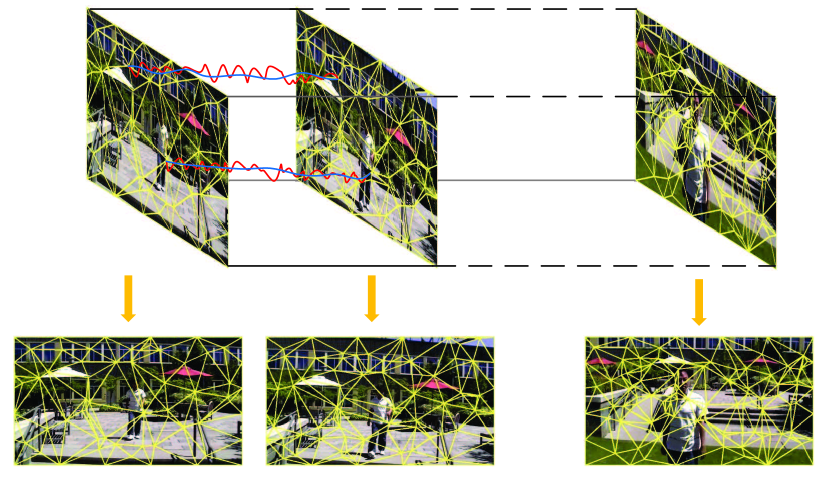
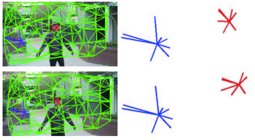
As shown in Fig. 1, we divide frames into triangle meshes according to the distribution of feature trajectories. These meshes have strong inter-frame correlation, i.e., the triangle meshes of neighboring frames are similar and vary slowly. This fact can help keep the local continuity of the adjacent stabilized frames and avoid sudden changes.
Based on the generated adaptive meshes, meshed transformations are calculated by solving a two-stage optimization problem. To further enhance the robustness of the obtained meshed transformations, two adaptive weighting mechanisms are proposed to improve the spatial and temporal adaptability.
The remainder of this paper is organized as follows. Section II presents the related work regarding video stabilization. Section III presents the details of our adaptively meshed video stabilization method and two adaptive weighting mechanisms. Section IV compares our method with some start-of-the-art stabilization methods through several public videos. Some concluding remarks are placed in Section V.
II Related Work
II-A Traditional Video Stabilization
Traditional video stabilization methods can be classified into three types, including 2D, 3D and 2.5D methods. 2D methods aim to stabilize videos mainly containing planar motion. Through image matching technologies, such as feature matching, 2D methods usually model the camera motion with inter-frame transformation matrix sequences [6], [7]. Under the assumption of static scenes, many smoothing techniques are implemented to smooth the obtained transformation matrices, such as Gaussian low-pass filtering [13], Particle filtering [14] and Regularization [15], then stabilized frames are generated with the smoothed transform matrices. Grundmann et al. [16] proposed a linear programming framework to calculate a global homography through minimizing the first, second and third derivatives of the resulting camera path. [17] extended the method of [16] by replacing the global homography with a homography array to reduce the rolling shutter distortion. Joshi et al. proposed a hyperlapse method [1], which optimally selects some frames from the input frames, ensures that the selected frames can best match a desired speed-up rate and also result in the smoothest possible camera motion, and stabilizes the video according to these selected frames. Meanwhile, Zhang et al. [9] introduced the “as-similar-as-possible” constraint to make the motion estimation more robust. 2D methods are computationally efficient and robust against planar camera motions, but may fail in the existence of strong parallax.
Parallax can be well handled by 3D methods. By detecting a set of feature points and tracking them at each frame, 3D methods reconstruct the 3D locations of these feature points and the 3D camera motion by the Structure-from-Motion (SFM) technique [11]. Thus these 3D methods are more complicated than 2D methods. Buehler et al. [18] got the smoothed locations of feature points by limiting the speed of the projected feature points to be constant. Liu et al. [2] developed a 3D content-preserving warping technique. In [19], video stabilization is solved with an additional depth sensor, such as a Kinect camera. Moreover, some plane constraints were introduced to improve video stabilization performance [20], [21]. Due to the implementation of SFM, 3D methods usually stabilize videos much slower than 2D methods and may be fragile in the case of planar motions.
2.5D methods combine the advantages of 2D methods and 3D methods. Liu et al. [22] extracted robust feature trajectories from the input frames and smoothed the camera path with subspace constraints. They also handled parallax by the content preserving warping [23]. As this subspace property may not hold for dynamic scenes where cameras move quickly, Goldstein et al. introduced epipolar constraints in [24] and employed time-view reprojection for foreground feature trajectories. In [25], Liu et al. designed a specific optical flow by enforcing strong spatial coherence and further extended it to meshflow [26] for sparse motion representation. However, these methods may fail when large foreground objects exist. So Ling et al. [27] took both foreground and background feature trajectories to estimate the camera jitters through solving an optimization problem. In [28], Zhao et al. implemented fast video stabilization assisted by foreground feature trajectories. Kon et al. [12] generated virtual trajectories by augmenting incomplete trajectories using a low-rank matrix completion scheme when the number of the estimated trajectories is insufficient. In [29], a novel method combines trajectory smoothing and frame warping into a single optimization framework and can conveniently increase the strength of the trajectory smoothing.
II-B CNN-based Video Stabilization
Recently convolutional neural networks(CNNs) were implemented for video stabilization. Wang et al. [10] built a novel video stabilization dataset, called DeepStab dataset which includes 61 pairs of stable and unstable videos, and designed a network for multi-grid warping transformation learning, which can achieve comparable performance as traditional methods in regular videos and is more robust for low-quality videos. In [30], adversarial networks are taken to estimate an affine matrix, with which steady frames can be generated. Huang et al. [31] designed a novel network which processes each unsteady frame progressively in a multi-scale manner from low resolution to high resolution, and then outputs an affine transformation to stabilize the frame. In [32], a framework with frame interpolation techniques is utilized to generate stabilized frames. Generally speaking, CNN-based methods have great potential to robustly stabilize various videos, but may be limited by the lack of training video datasets.
III Proposed Method
As a 2.5D method, our method estimates the camera motion, smooths it and generates stabilized frames based on feature trajectories. Compared with previous 2.5D methods, which handle parallax and discontinuous depth variation caused by foreground objects with fixed meshes, our method adaptively adjusts meshes by an adaptive blocking strategy and works well against different complicated scenes. In the following subsections, we first introduce the feature trajectory pre-processing and related mathematical definitions, then will present the key steps of the proposed method.
III-A Pre-processing and mathematical definitions
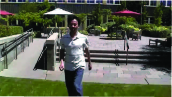
We adopt the KLT tracker of [33] to detect feature points at each frame and track them to generate feature trajectories. To avoid all feature trajectories gathering in some small regions, we first divide each video frame into 10 by 10 grids and detect 200 corners with a global threshold. For grids which have no detected corners, we will decrease their local thresholds to ensure that at least one corner can be detected in each grid. Then these corners are tracked to generate feature trajectories. Thus there will be more feature trajectories in the grids with rich contents while less corners in grids with poor contents. As [29], the corner detection procedure is executed only when the number of tracked feature points decreases to a certain level. However, in our method, much fewer corners are detected (1000 corners in [29]) since we directly produce the triangle mesh according to the positions of feature trajectories in each frame. We keep all trajectories whose length is longer than 3 frames.
Suppose there are feature trajectories in a shaky video, which are denoted as . These feature trajectories may come from either the background or foreground objects. Denote the first and last frames, in which trajectory () appears, as and . Denote the feature point of trajectory at frame () as . The feature points of all feature trajectories which appear at frame are grouped into a set,
| (1) |
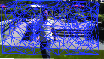
Then we generate a triangle mesh of frame with through standard constrained Delaunay triangulation[34], which is illustrated in Fig. 2(b). Suppose there are triangles in the triangle mesh of frame , then the set of triangles of frame is denoted as . The stabilized views of and are represented as and , respectively.
Our method estimates , i.e., the stabilized views of feature trajectories , through solving an optimization problem under the following three constraints.
-
1.
For a given feature trajectory , its stabilized view should vary slowly.
-
2.
At frame , each stabilized triangle is geometrically similar to its original triangle .
-
3.
At frame , the transformations between and its adjacent triangles should be similar to the corresponding transformations between and its adjacent triangles.
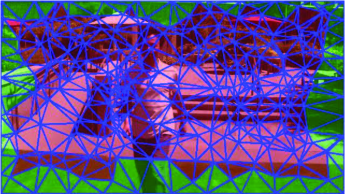
As shown in Fig. 2(b), all triangles are constructed with feature trajectories and we can calculate their stabilized views and warp these regions according to the corresponding transformations. At each frame, our method also evenly sets (other number should also be fine) control points on each of four frame edges and produces control points which are denoted as . Then we divide frame with the new set through Delaunay triangulation to produce a triangle mesh. The obtained triangle mesh is represented as , where , called inner triangles, are triangles whose vertices are made up of only , and , called outer triangles, are triangles whose vertices contain at least one control point. In Fig. 2(c), inner triangles are presented in red and outer triangles in green. Then a two-stage optimization problem is solved to calculate and , i.e., the stabilized views of and . At the first stage, a global optimization problem is solved to estimate the stabilized views of feature trajectories , i.e., , which form as (1). At the second stage, a frame-by-frame optimization problem is solved to produce . Finally, each frame is warped through the transformations between the triangles generated by and the ones by .
III-B Stabilized view estimation from feature trajectories
Based on the three constraints in Section III-A, the stabilized view of is obtained through solving the following optimization problem,
| (2) |
where
is the smoothing term to smooth feature trajectories, is the inter-frame similarity transformation term to ensure that the warped frame closely follows the similarity transformation of its original frame, is the intra-frame similarity transformation term to ensure that the similarity transformation between adjacent regions of a stabilized frame is close to the corresponding transformation of its original frame, and is the regularization term to avoid too much warping. The details of these four terms are provided below.
III-B1 The smoothing term
Motivated by [16], we smooth the feature trajectories through their first-order and second-order derivatives. The first-order derivative term requires each stabilized feature trajectory to change slowly, i.e., we expect
| (4) |
If this requirement is satisfied, the camera will be static and the generated video will be the most stable. However, that extreme requirement may cause much cropping and discard a lot of contents of the video. So we introduce the second-derivative term, which requires the velocity of each feature trajectory to be constant, i.e.,
| (5) |
The term in (5) will limit the change of the inter-frame motion and produce stable feature trajectories. Combining the first-order derivative term and the second-order derivative term, we define as
| (6) | |||||
where and are weighting parameters to be determined later.
III-B2 The inter-frame similarity transformation term
This term is designed by following the “as-similar-as-possible” warping method of [2]. For Delaunay triangles in , their stabilized views are denoted as . The vertices of triangle in and are denoted as and , respectively. To preserve the local shape of frame , is required to be geometrically similar to . As shown in Fig. 3, for triangle in , any vertex can be locally represented by the other two vertices. For example, we have
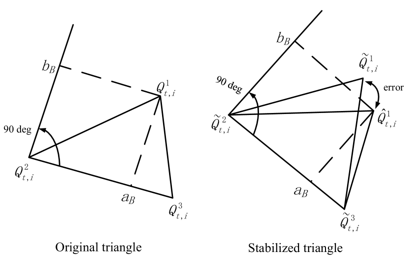
| (7) |
where , and and are the coordinates of in the local coordinate system defined by and . Based on the geometric similarity constraint between and , the expected position of is
| (8) |
Our goal is to minimize . Similar constraints are performed for and and the overall inter-frame similarity transformation term is defined as
| (9) |
where is the total number of frames of the concerned video. Note that since is made up of , the constraints for is equivalent to the constraints for , which is actually the set of feature points of stabilized trajectories at each frame.
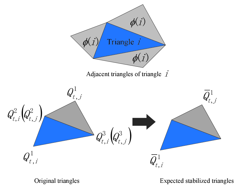
III-B3 The intra-frame similarity transformation term
To avoid distortion in stabilized frames, this term requires that the transformations between adjacent regions in each stabilized frame should be closely followed by those corresponding transformations in its original frame. As shown in Fig. 4, in the triangle mesh, each triangle and its adjacent triangles share one common edge. For triangle at frame , we take one of its neighbors, triangle , as an example. Triangles and share two vertices which are denoted as and , while the other vertices of the two triangles are and , respectively. Then can be represented by the coordinates of triangle through the standard linear texture mapping [34],
| (13) |
where and are the horizontal and vertical components of , , and are weighting parameters. With these weights, , and , the expected position of is calculated as
| (14) |
In order to ensure the transformation between and is close to the one between and , we want to minimize the difference between and its stabilized coordinate , i.e.,
| (15) |
Similarly, we can calculate and reduce the difference between and . The total intra-frame similarity transformation term is defined as
| (16) |
where is the set of adjacent triangles of triangle , and is a weighting parameter to be determined later.
III-B4 The regularization term
aims to regularize the optimization in (III-B) so that the stabilized trajectories stay close to their original ones to avoid too much warping. It is defined as
| (17) |
With the above optimization in (III-B), we can get the stabilized views of all feature trajectories, i.e., ().
III-C Stabilized view estimation from control points
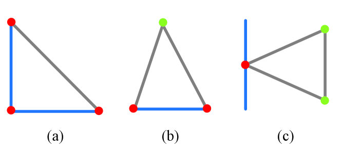
Given the stabilized views of feature trajectories, , we have the stabilized views of and at each frame, i.e., and . At each frame, we estimate the stabilized view of control points , i.e., , by solving an optimization problem. Then the stabilized view of , , can be computed from and . Finally, each frame is warped according to the transformations between and . There are three types of triangles in , triangles with , or control points, which are shown in Fig. 5. We design an optimization problem to calculate only the stabilized views of control points in as follows,
| (18) |
where
| (19) |
and the definitions of and are given below.
III-C1 The inter-frame similarity transformation term
This term is also designed to ensure that is geometrically similar to . For triangle in , we have
| (20) |
where , and and are the coordinates of in the local coordinate system defined by and . Based on the geometric similarity constraint between and , the expected position of is
| (21) |
Here may contain one or two vertices, which also belong to triangles of . These common vertices have been calculated by (2) and do not need to be optimized again. Therefore, in (21), we replace these common vertices of , denoted as , with the corresponding stabilized vertices in triangles of , which are denoted as . So the inter-frame similarity transformation term is defined as
| (22) |
where is a weighting parameter to be determined later, and is defined as
| (25) | |||
| (26) |
III-C2 The intra-frame similarity transformation term
This term is similar to in Section III-B3. Transformations between adjacent triangles in each stabilized frame are also expected to be close to the corresponding transformations between adjacent triangles in its original frame. Note that the adjacent triangle of triangle may come from or . We simply combine and into a larger set, which is denoted as , and the adjacent triangle of is denoted as at frame . The different vertices of and are denoted as and . Then can be represented by the coordinates of triangle through the linear texture mapping
| (27) |
where , and can be similarly calculated as (13). The expected coordinate with these weights and corresponding vertices of the stabilized triangle , i.e., , , , are calculated as
| (28) |
is expected to stay close to the stabilized coordinate . When vertices of and belong to some triangles of , these common vertices are replaced with the stabilized vertices of the corresponding triangles of .
Similarly, we have and . is expected to stay close to . Finally the intra-frame similarity transformation term is defined as
| (29) |
where is the same weighting parameter in (16), is defined as
| (32) | |||
| (33) |
and is similarly defined as .
III-D Adaptive Weighting Mechanisms
To enhance the robustness of our method, we further introduce two adaptive weighting mechanisms to adjust the weighting parameters of the optimization in (III-B). They aim to improve the spatial and temporal adaptability of our method.
III-D1 A weighting mechanism to improve the temporal adaptability
According to the analysis in [29], aims to reduce the inter-frame movement of a trajectory to zero. However, the fast camera motion usually produces huge inter-frame movement of feature trajectories. is enforced to reduce such inter-frame movement; otherwise, too big inter-frame movement may lead to the collapse of the stabilization of shaky videos. So the weight of the first-order derivative term in (6), i.e., , should be reduced when the camera moves fast. Different from the method of [29], we consider the speed continuity of the camera motion, and update into
| (34) | |||||
where and are the horizontal and vertical components of , and and are the horizontal and vertical components of . and measure the inter-frame movement of feature trajectory at frame and are calculated as and . is a constant. When the camera moves fast, decreases so that the smoothing strength of is reduced. This adaptive weighting mechanism enables our method to handle videos with fast camera motion. An example in Fig. 6 shows the effects of this weighting mechanism on the temporal adaptability.
III-D2 A weighting mechanism to improve the spatial adaptability
During stabilizing shaky videos, we cannot ignore discontinuous depth variation or different local motion caused by foreground objects; otherwise, significant distortion may appear in stabilized frames. To solve this problem, we first determine whether each triangle of the triangle mesh contains foreground objects or not, and then increase the weights of triangles containing foreground objects inside of (III-B). This operation will avoid serious distortion artifacts in complicated scenes and enhance the robustness of our optimization model.
Given a feature point in at frame , and its neighboring feature points comprise a set , where is point . As shown in Fig. 7, if all points in belong to the background, their arrangement at adjacent frames is similar. However, when some points in belong to the foreground, their arrangement may change much at adjacent frames. So we take the arrangement change to judge the existence of foreground objects and adjust the weight of in the proposed optimization problem. Specifically, for feature trajectory , we calculate the transformation between and by solving the overdetermined equation in (26) with
| (26) |
| (27) |
(26) can be solved by the least square method. (26) can be abbreviated into and provide the solution of with the following residual error
where measures the weight of the point set and is defined as
| (29) |
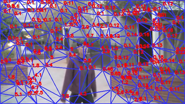
where , and are the width and height of the video frame, is used to control the block size in the normalization and is set to 10 here. To control the influence of in the proposed optimization problem, is limited into the range of . Fig. 8 shows in an example frame. It can be seen that large usually appears at the feature points related to foreground objects while in the background is usually small.
Finally we update into
| (30) |
where stands for the set of 3 vertices of triangle .
IV Experimental Results
IV-A Dataset and Evaluation Metrics
To verify the performance of our method, we collected 36 typical videos from public datasets111 http://liushuaicheng.org/SIGGRAPH2013/database.html,
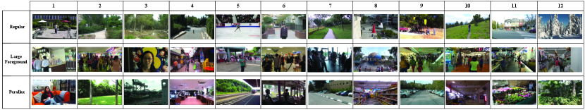
http://web.cecs.pdx.edu/~fliu/project/subspace_stabilization/. . These videos can be classified into three categories, including “ Regular”, “Large foreground” and “Parallax”, which are shown in Fig. 9. “Regular” category contains several regular videos recording some common scenes. “Large foreground” category contains several videos where large foreground objects occupy a large part of video frames and cause serious discontinuous depth variation. “Parallax” means there is strong parallax in the captured scenes of the videos. The last two categories are more challenging and their experiments confirm that our method can achieve much better performance than previous works.
For quantitative comparison, we consider two evaluation metrics: Stability score and SSIM.
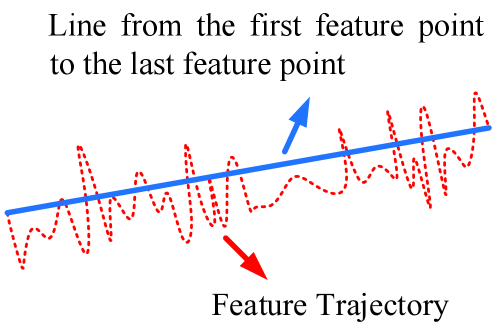
Stability score: This metric is taken from [35]. As shown in Fig. 10, the red dotted curve represents a feature trajectory, and the blue line directly connects the start point and the end point of the feature trajectory. Then the stability score is defined as the length of the blue line divided by that of the red dotted curve. The range of stability score is (0,1], and a larger value means a more stable result. Following [29], feature trajectories are extracted by the KLT tracker and are divided into segments of the length of 40 frames. We ignore segments whose lengths are less than 40 frames. The final stability score of a stabilized video is defined as the average stability score of all segments.
SSIM: SSIM (structural similarity) [36] is a widely-used index to measure the video stabilization performance. This index combines luminance, contrast and structure comparison to calculate the similarity of two given images. We calculate the SSIM of every two adjacent frames in a video and average them to produce the final SSIM value of a video.
IV-B Ablation Study
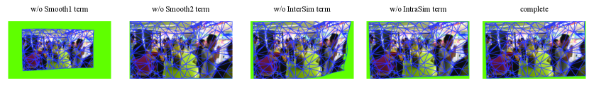
Here we first perform ablation study to evaluate the effectiveness of terms of our proposed optimization framework in (2). To analyze the importance of each term in (III-B), we remove one term of (III-B) at a time and then evaluate the stabilization performance. The quantitative and qualitative results are shown in Fig. 11 and Table I.
Among all terms in (III-B), we do not check the influence of the regularization term as it is a basic term to make sure that the stabilized trajectories stay close to their original ones and are free of drift. For the other terms, we remove one term from the performance index by setting its weight to zero, i.e., one of , , and is set to . Table I shows the quantitative results of the ablation study where both the stability score and SSIM are calculated. Fig. 11 shows the visualization results of the ablation study. In Table I, we find that without , the stability performance is seriously degraded, which confirms that the first-order derivative term is the main one to guarantee the low-frequency characteristics of the stabilized videos. The stability score and SSIM also degrade when the second-order derivative term is removed from the optimization function. According to the analysis in Section III-D1, removing the second-order derivative term means that feature trajectories are smoothed only with the first-order derivative term and the camera motion is enforced to be static. Thus fast camera movement may yield artifacts and even collapse, which is demonstrated in Fig. 11. also significantly influences the performance. As shown in Fig. 11, due to the lack of the local shape preserving constraint, serious distortion may happen when parallax or large foreground objects exist, which also cause the non-smoothing of stabilized videos. Table I also shows that when is removed, the stabilization performance becomes worse, which illustrates the importance of this term in keeping the similar transformation in the adjacent regions. can also avoid the trajectory mis-matching and improve the stabilization results.
| Metrics | Stability Score | SSIM | ||||
| Optimization Terms | Regular | Large foreground | Parallax | Regular | Large foreground | Parallax |
| w/o Smooth0 | 0.7998 | 0.7657 | 0.7821 | 0.7045 | 0.7663 | 0.7433 |
| w/o Smooth1 | 0.8241 | 0.7895 | 0.8268 | 0.7520 | 0.7997 | 0.7965 |
| w/o InterSim | 0.8407 | 0.8027 | 0.8304 | 0.7609 | 0.8002 | 0.7920 |
| w/o IntraSim | 0.8514 | 0.8178 | 0.8356 | 0.7664 | 0.8046 | 0.7969 |
| complete | 0.8589 | 0.8287 | 0.8541 | 0.7750 | 0.8196 | 0.8033 |
IV-C Comparison with Previous Methods
We compare our method with several state-of-the-art methods, including Subspace [22], Meshflow [26], Deep learning [10], Effective [29] and Global [37]. Subspace is implemented in Adobe Premiere stabilizer. The codes of Meshflow [26], Deep learning [10] and Effective [29] were found at https://github.com/sudheerachary/Mesh-Flow-Video-Stabilization, https://github.com/cxjyxxme/deep-online-video-stabilization-deploy and https://github.com/705062791/TVCG-Video-Stabilization-via-joint-Trajectory-Smoothing-and-frame-warping. Thanks to the authors of[37], who provided us with the binary implementation of Global.
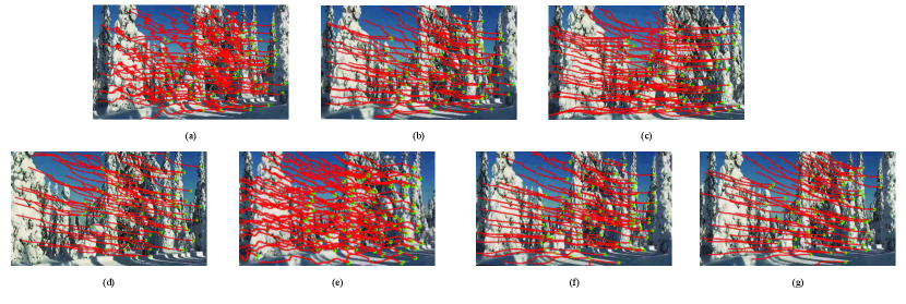
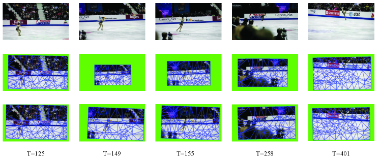
Here we first compare our method with these methods through some qualitative results, which are shown in Fig. 12 and Fig. 13. Fig. 12 shows feature trajectories of an example shaky video and the corresponding stabilized videos. The Deep learning method stabilizes videos without using future frames. Therefore, compared with other methods, its stabilization effect is the worst. Although the Effective method reduces most of high-frequency shakiness, we can still catch many visible low-frequency footstep motions. Therefore, its trajectories are not good enough. The results of the Subspace, Meshflow and Global methods eliminate almost all high-frequency shakiness, and generate similar stabilization effects. The results of the proposed method show significant improvement, which is confirmed by the smoothness of the stabilized trajectories.
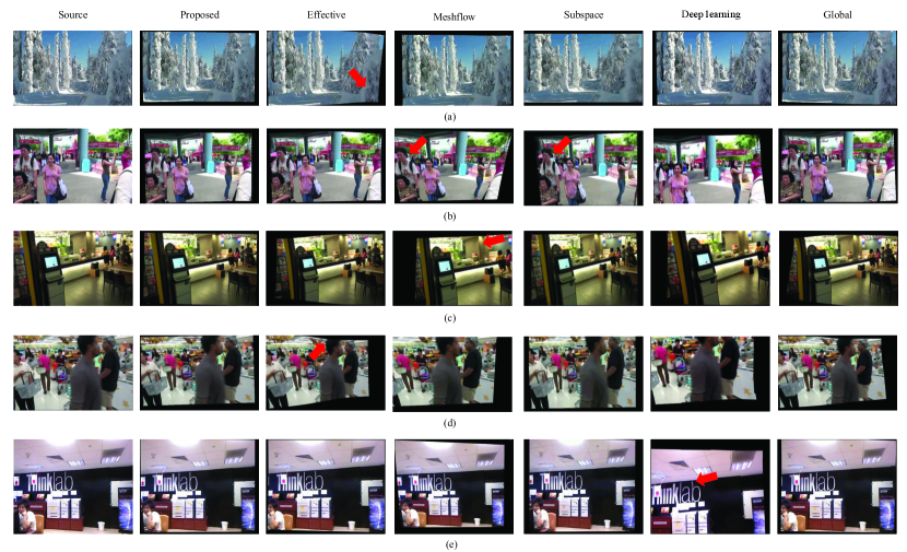
In addition to stability, noticeable visual distortion should also be avoided in stabilized videos. Fig. 13 shows some example frames in several stabilized videos by different methods. The Subspace method performs motion compensation through smoothing long feature trajectories with low-rank constraints. As shown by Fig. 13(b), when there are not enough long feature trajectories, for example, in the case of fast moving foreground objects, Subspace may fail and result in serious distortion. The Meshflow and Global methods discard foreground feature trajectories and estimate the camera motion with only the background feature trajectories. However, separating foreground trajectories from background ones is a difficult task, especially in large foreground scenes or strong parallax. So these methods may suffer performance degradation in challenging videos, as shown by Fig. 13(b) and 13(c). The Deep learning method stabilizes videos without future frames and regresses one homography for each of fixed grids. The inaccurate estimation and weak constraint for local shape preserving may incur noticeable distortion, which is illustrated in Fig. 13(e). The Effective method estimates the camera motion based on all feature trajectories. However, this method divides frames into fixed mesh grids of the same size and extract a similar number of feature trajectories in each mesh grid, which is not reasonable for complicated scenes, such as large foreground and parallax. Fig. 13(a) and 13(d) show that this method may cause distortion in regions with rich contents or large depth variation.
The quantitative comparison on all test videos is also performed. Table II and Table III show Stability score and SSIM generated by different methods on all test videos. In terms of Stability score, the proposed method outperforms all other methods on most videos in the “Regular” category. Only in two videos, the Subspace method gets the highest Stability score, which is slightly better than that of the proposed method. However, the Subspace method gets worse results than some other methods in other videos. More significant performance improvement of the proposed method can be observed in the other two complicated categories, “Large foreground” and “Parallax”. Our method gets much higher Stability scores on most videos. Note that the compared methods, except the Subspace method, take fixed meshes in stabilizing videos. For the scenes containing large foreground objects or parallax, these methods may suffer serious performance degradation while our method can get much better results with the adaptively adjusted mesh. Moreover, the proposed method takes both background feature trajectories and foreground feature trajectories to smooth the camera motion and may be hardly disturbed by the active motion of the foreground objects. Thus the proposed method achieves higher Stability scores in most videos than the methods which discard foreground feature trajectories. So our method is the most robust among all methods. Similar SSIM comparison results can also be observed in Table III. The proposed method gets much better stability score and SSIM in most videos than other methods. Since stability score measures the stability of local feature trajectories and SSIM measures the global similarity of adjacent frames in the stabilized videos, the results confirm the effectiveness of our method. For more thorough comparison, a supplemental demo is provided at http://home.ustc.edu.cn/~zmd1992/content-aware-stabilization.html.
| Regular | Methods | 1 | 2 | 3 | 4 | 5 | 6 | 7 | 8 | 9 | 10 | 11 | 12 |
| Effective [29] | 0.7529 | 0.7483 | 0.9292 | 0.6516 | 0.7161 | 0.8201 | 0.6965 | 0.7141 | 0.7413 | 0.624 | 0.8022 | 0.9036 | |
| Meshflow [26] | 0.7295 | 0.8298 | 0.9260 | 0.7272 | 0.8137 | 0.8247 | 0.6564 | 0.7069 | 0.7813 | 0.5147 | 0.8061 | 0.9151 | |
| Subspace [22] | 0.6633 | 0.9049 | 0.9515 | 0.8328 | 0.6552 | 0.4191 | 0.7281 | 0.5866 | 0.8526 | 0.4527 | 0.6165 | 0.8270 | |
| Deep learning [10] | 0.4056 | 0.5601 | 0.6825 | 0.4454 | 0.6679 | 0.6007 | 0.4299 | 0.2597 | 0.5572 | 0.4200 | 0.5353 | 0.7781 | |
| Global [37] | 0.8282 | 0.8791 | 0.9650 | 0.7779 | 0.7347 | 0.8441 | 0.6432 | 0.7739 | 0.7915 | 0.6808 | 0.7846 | 0.928 | |
| Proposed | 0.8559 | 0.8974 | 0.9686 | 0.8372 | 0.8578 | 0.8513 | 0.8096 | 0.8138 | 0.8334 | 0.7810 | 0.8578 | 0.9437 | |
| Large foreground | Methods | 1 | 2 | 3 | 4 | 5 | 6 | 7 | 8 | 9 | 10 | 11 | 12 |
| Effective [29] | 0.8189 | 0.7241 | 0.5980 | 0.7169 | 0.8049 | 0.7149 | 0.7222 | 0.8387 | 0.7253 | 0.7322 | 0.8257 | 0.7782 | |
| Meshflow [26] | 0.8495 | 0.7197 | 0.6082 | 0.7326 | 0.7542 | 0.7404 | 0.8167 | 0.8376 | 0.7442 | 0.7427 | 0.8198 | 0.7891 | |
| Subspace [22] | 0.5884 | 0.6768 | 0.4784 | 0.6685 | 0.6525 | 0.6130 | 0.7071 | 0.5659 | 0.3239 | 0.6130 | 0.7747 | 0.6698 | |
| Deep learning [10] | 0.3437 | 0.3832 | 0.4764 | 0.4690 | 0.4371 | 0.4760 | 0.6218 | 0.5000 | 0.5242 | 0.6430 | 0.5544 | 0.4960 | |
| Global [37] | 0.7575 | 0.4076 | 0.6167 | 0.6213 | 0.7679 | 0.6505 | 0.8395 | 0.8633 | 0.6253 | 0.6953 | 0.7827 | 0.7411 | |
| PROPOSED | 0.8901 | 0.7903 | 0.6305 | 0.8249 | 0.8652 | 0.8064 | 0.8369 | 0.8893 | 0.8161 | 0.8422 | 0.8841 | 0.8690 | |
| Parallax | Methods | 1 | 2 | 3 | 4 | 5 | 6 | 7 | 8 | 9 | 10 | 11 | 12 |
| Effective [29] | 0.8315 | 0.8498 | 0.7044 | 0.7447 | 0.8544 | 0.7371 | 0.6895 | 0.9412 | 0.7450 | 0.7600 | 0.8716 | 0.4855 | |
| Meshflow [26] | 0.8082 | 0.9039 | 0.7170 | 0.7162 | / | / | 0.6729 | 0.6398 | 0.8021 | 0.7957 | 0.8682 | 0.5898 | |
| Subspace [22] | 0.8112 | 0.9125 | 0.4767 | 0.6697 | 0.8854 | 0.8035 | 0.8272 | 0.9174 | 0.8963 | 0.7942 | 0.9170 | 0.5100 | |
| Deep learning [10] | 0.6140 | 0.7561 | 0.5496 | 0.6442 | 0.5768 | 0.5684 | 0.5246 | 0.5950 | 0.4338 | 0.4314 | 0.7110 | 0.3455 | |
| Global [37] | 0.8089 | 0.5740 | 0.6862 | 0.8052 | 0.7635 | 0.7453 | 0.7519 | / | 0.8675 | 0.8204 | 0.8905 | 0.6501 | |
| PROPOSED | 0.8648 | 0.9111 | 0.7663 | 0.8549 | 0.8983 | 0.8216 | 0.8291 | 0.9238 | 0.9076 | 0.8444 | 0.9059 | 0.7208 |
| Regular | Methods | 1 | 2 | 3 | 4 | 5 | 6 | 7 | 8 | 9 | 10 | 11 | 12 |
| Effective [29] | 0.8026 | 0.6804 | 0.5647 | 0.8195 | 0.8004 | 0.6913 | 0.7781 | 0.8874 | 0.8755 | 0.7693 | 0.7507 | 0.5814 | |
| Meshflow [26] | 0.8260 | 0.6815 | 0.4919 | 0.8423 | 0.8363 | 0.6986 | 0.8084 | 0.9042 | 0.8690 | 0.7440 | 0.7658 | 0.5257 | |
| Subspace [22] | 0.5637 | 0.6895 | 0.4587 | 0.8443 | 0.8328 | 0.6159 | 0.7608 | 0.6056 | 0.8604 | 0.6546 | 0.5462 | 0.4679 | |
| Deep learning [10] | 0.7133 | 0.6638 | 0.5597 | 0.7666 | 0.7371 | 0.6477 | 0.6627 | 0.7813 | 0.8636 | 0.7037 | 0.6656 | 0.5831 | |
| Global [37] | 0.7943 | 0.6101 | 0.4388 | 0.7752 | 0.7912 | 0.6569 | 0.7403 | 0.8764 | 0.8558 | 0.7192 | 0.7518 | 0.5566 | |
| PROPOSED | 0.8447 | 0.6712 | 0.6171 | 0.8461 | 0.8009 | 0.7434 | 0.8141 | 0.9240 | 0.9083 | 0.8004 | 0.8301 | 0.6000 | |
| Large foreground | Methods | 1 | 2 | 3 | 4 | 5 | 6 | 7 | 8 | 9 | 10 | 11 | 12 |
| Effective [29] | 0.6771 | 0.7365 | 0.8261 | 0.6815 | 0.7213 | 0.7657 | 0.7057 | 0.6525 | 0.7579 | 0.7096 | 0.7135 | 0.6774 | |
| Meshflow [26] | 0.7450 | 0.7978 | 0.8545 | 0.7423 | 0.7596 | 0.8132 | 0.7470 | 0.6852 | 0.8275 | 0.7746 | 0.782 | 0.7458 | |
| Subspace [22] | 0.4738 | 0.6359 | 0.6890 | 0.5127 | 0.623 | 0.7176 | 0.6144 | 0.5072 | 0.4916 | 0.5212 | 0.5182 | 0.5679 | |
| Deep learning [10] | 0.5223 | 0.5935 | 0.7977 | 0.5830 | 0.6056 | 0.6747 | 0.6396 | 0.5525 | 0.6337 | 0.6409 | 0.6336 | 0.5815 | |
| Global [37] | 0.7270 | 0.5711 | 0.8164 | 0.7101 | 0.7502 | 0.7953 | 0.7191 | 0.6639 | 0.7966 | 0.7593 | 0.7625 | 0.7360 | |
| PROPOSED | 0.7999 | 0.8379 | 0.8573 | 0.7955 | 0.8226 | 0.8638 | 0.7985 | 0.7540 | 0.8588 | 0.8266 | 0.8260 | 0.7948 | |
| Parallax | Methods | 1 | 2 | 3 | 4 | 5 | 6 | 7 | 8 | 9 | 10 | 11 | 12 |
| Effective [29] | 0.7351 | 0.6109 | 0.8721 | 0.7459 | 0.7744 | 0.8065 | 0.8788 | 0.5493 | 0.8822 | 0.9048 | 0.6441 | 0.8677 | |
| Meshflow [26] | 0.7420 | 0.6297 | 0.9006 | 0.7219 | / | / | 0.8649 | 0.5550 | 0.8903 | 0.9299 | 0.6312 | 0.8850 | |
| Subspace [22] | 0.6877 | 0.4779 | 0.8544 | 0.7544 | 0.7769 | 0.7889 | 0.8949 | 0.5324 | 0.8987 | 0.9251 | 0.6242 | 0.7845 | |
| Deep learning [10] | 0.7261 | 0.5278 | 0.8431 | 0.6896 | 0.7872 | 0.6933 | 0.7749 | 0.4332 | 0.7882 | 0.8555 | 0.5920 | 0.8531 | |
| Global [37] | 0.7143 | 0.7005 | 0.8793 | 0.7428 | 0.7879 | 0.7764 | 0.8614 | / | 0.8640 | 0.8660 | 0.6423 | 0.8243 | |
| PROPOSED | 0.7740 | 0.6732 | 0.9141 | 0.7808 | 0.8278 | 0.8441 | 0.8998 | 0.5667 | 0.9021 | 0.9130 | 0.6558 | 0.8889 |
IV-D Parameter Sensitivity
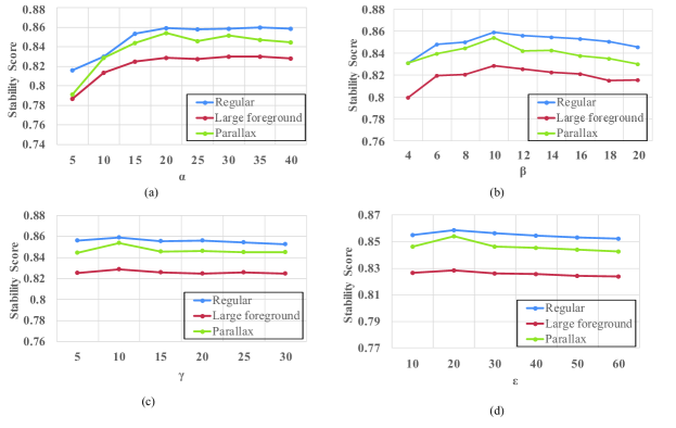
Here we investigate the parameter sensitivity of the proposed method. Since the weight of is normalized to 1, there are four parameters, including , , and , which are the weights of , , and , respectively. For one term, a larger weight implies more importance.
Each time we change one weight, fix the others and calculate the average stability scores on three categories to quantitatively measure its sensitivity.
-
•
Fig. 14(a) shows the influence of , where varies from 5 to 40. We find that when is smaller than 20, the performance becomes obviously better as increases. When is large than 20, the stability score will slightly increase. However, according to the previous analysis, too large will result in serious collapse risk. So is set to 20.
-
•
As shown in Fig. 14(b), when increases from 4 to 20, the stability score first increases and then decreases on all three categories. Note that both the increasing amount and the decreasing amount of the stability score are small. So the stabilization performance is not much sensitive to . is set to 10.
-
•
The results under various and are shown in Fig. 14(c) and Fig. 14(d). When and increase, the stability scores first slightly increase and then slowly decrease, which means the stabilization performance is not sensitive to or . Note that increasing and is equivalent to decreasing the weights of two smoothing terms, i.e., and . and are set to 10 and 20, respectively.
V Conclusion
In this paper, we propose an adaptively meshed video stabilization method. Different from previous works, which stabilize shaky videos based on fixed meshes, we propose a novel stabilization method by considering the contents of the video and adaptively dividing each frame into a flexible number of mesh grids. The adaptive blocking strategy is realized by the Delaunay triangulation of feature trajectories and all mesh grids are triangles with various sizes. The stabilized views of all triangles in the triangle mesh are calculated through solving a two-stage optimization problem. The proposed method takes both foreground feature trajectories and background feature trajectories for precise jitter estimation. To further enhance the robustness of our method, we propose two adaptive weighting mechanisms to improve the spatial and temporal adaptability. Experiments on several public videos confirm the performance superiority of our method.
There are two main limitations of the proposed method. The first one is its computational burden. Our method takes an average of 0.3s to process one frame, which is slower than some previous works, such as Meshflow [26] and Global [37]. The further acceleration of the proposed method will be pursued in the future. The other limitation is also common for other traditional video stabilization methods, i.e., the video stabilization is built upon feature trajectories and may be fragile for low-quality videos with non-texture scenes where it is hard to extract an enough number of reliable feature trajectories. Some deep learning based methods have been proposed to solve this problem, such as [10] and [30]. We will keep eyes on that direction.
References
- [1] N. Joshi, W. Kienzle, M. Toelle, M. Uyttendaele, and M. F. Cohen, “Real-time hyperlapse creation via optimal frame selection,” ACM Transactions on Graphics (TOG), vol. 34, no. 4, p. 63, 2015.
- [2] F. Liu, M. Gleicher, H. Jin, and A. Agarwala, “Content-preserving warps for 3d video stabilization,” in ACM Transactions on Graphics (TOG), vol. 28, no. 3. ACM, 2009, p. 44.
- [3] N. Gard, A. Hilsmann, and P. Eisert, “Projection distortion-based object tracking in shader lamp scenarios,” IEEE transactions on visualization and computer graphics, vol. 25, no. 11, pp. 3105–3113, 2019.
- [4] L. Wang, Y. Xiong, Z. Wang, Y. Qiao, D. Lin, X. Tang, and L. Van Gool, “Temporal segment networks: Towards good practices for deep action recognition,” in European conference on computer vision. Springer, 2016, pp. 20–36.
- [5] M. Liu, J. Shi, Z. Li, C. Li, J. Zhu, and S. Liu, “Towards better analysis of deep convolutional neural networks,” IEEE transactions on visualization and computer graphics, vol. 23, no. 1, pp. 91–100, 2016.
- [6] B.-Y. Chen, K.-Y. Lee, W.-T. Huang, and J.-S. Lin, “Capturing intention-based full-frame video stabilization,” in Computer Graphics Forum, vol. 27, no. 7. Wiley Online Library, 2008, pp. 1805–1814.
- [7] M. L. Gleicher and F. Liu, “Re-cinematography: Improving the camerawork of casual video,” ACM transactions on multimedia computing, communications, and applications (TOMM), vol. 5, no. 1, p. 2, 2008.
- [8] C. Morimoto and R. Chellappa, “Evaluation of image stabilization algorithms,” in Proceedings of the 1998 IEEE International Conference on Acoustics, Speech and Signal Processing, ICASSP’98 (Cat. No. 98CH36181), vol. 5. IEEE, 1998, pp. 2789–2792.
- [9] L. Zhang, Q. Zheng, and H. Huang, “Intrinsic motion stability assessment for video stabilization,” IEEE transactions on visualization and computer graphics, vol. 25, no. 4, pp. 1681–1692, 2018.
- [10] M. Wang, G.-Y. Yang, J.-K. Lin, S.-H. Zhang, A. Shamir, S.-P. Lu, and S.-M. Hu, “Deep online video stabilization with multi-grid warping transformation learning,” IEEE Transactions on Image Processing, vol. 28, no. 5, pp. 2283–2292, 2018.
- [11] R. Hartley and A. Zisserman, Multiple view geometry in computer vision. Cambridge university press, 2003.
- [12] Y. J. Koh, C. Lee, and C.-S. Kim, “Video stabilization based on feature trajectory augmentation and selection and robust mesh grid warping,” IEEE Transactions on Image Processing, vol. 24, no. 12, pp. 5260–5273, 2015.
- [13] Y. Matsushita, E. Ofek, W. Ge, X. Tang, and H.-Y. Shum, “Full-frame video stabilization with motion inpainting,” IEEE Transactions on Pattern Analysis & Machine Intelligence, no. 7, pp. 1150–1163, 2006.
- [14] J. Yang, D. Schonfeld, and M. Mohamed, “Robust video stabilization based on particle filter tracking of projected camera motion,” IEEE Transactions on Circuits and Systems for Video Technology, vol. 19, no. 7, pp. 945–954, 2009.
- [15] H.-C. Chang, S.-H. Lai, and K.-R. Lu, “A robust and efficient video stabilization algorithm,” in 2004 IEEE International Conference on Multimedia and Expo (ICME)(IEEE Cat. No. 04TH8763), vol. 1. IEEE, 2004, pp. 29–32.
- [16] M. Grundmann, V. Kwatra, and I. Essa, “Auto-directed video stabilization with robust l1 optimal camera paths,” in CVPR 2011. IEEE, 2011, pp. 225–232.
- [17] M. Grundmann, V. Kwatra, D. Castro, and I. Essa, “Calibration-free rolling shutter removal,” in 2012 IEEE international conference on computational photography (ICCP). IEEE, 2012, pp. 1–8.
- [18] C. Buehler, M. Bosse, and L. McMillan, “Non-metric image-based rendering for video stabilization,” in Proceedings of the 2001 IEEE Computer Society Conference on Computer Vision and Pattern Recognition. CVPR 2001, vol. 2. IEEE, 2001, pp. II–II.
- [19] S. Liu, Y. Wang, L. Yuan, J. Bu, P. Tan, and J. Sun, “Video stabilization with a depth camera,” in 2012 IEEE Conference on Computer Vision and Pattern Recognition. IEEE, 2012, pp. 89–95.
- [20] Z.-Q. Wang, L. Zhang, and H. Huang, “Multiplane video stabilization,” in Computer Graphics Forum, vol. 32, no. 7. Wiley Online Library, 2013, pp. 265–273.
- [21] Z. Zhou, H. Jin, and Y. Ma, “Plane-based content preserving warps for video stabilization,” in Proceedings of the IEEE Conference on Computer Vision and Pattern Recognition, 2013, pp. 2299–2306.
- [22] F. Liu, M. Gleicher, J. Wang, H. Jin, and A. Agarwala, “Subspace video stabilization,” ACM Transactions on Graphics (TOG), vol. 30, no. 1, p. 4, 2011.
- [23] Y.-S. Wang, F. Liu, P.-S. Hsu, and T.-Y. Lee, “Spatially and temporally optimized video stabilization,” IEEE transactions on visualization and computer graphics, vol. 19, no. 8, pp. 1354–1361, 2013.
- [24] A. Goldstein and R. Fattal, “Video stabilization using epipolar geometry,” ACM Transactions on Graphics (TOG), vol. 31, no. 5, p. 126, 2012.
- [25] S. Liu, L. Yuan, P. Tan, and J. Sun, “Steadyflow: Spatially smooth optical flow for video stabilization,” in Proceedings of the IEEE Conference on Computer Vision and Pattern Recognition, 2014, pp. 4209–4216.
- [26] S. Liu, P. Tan, L. Yuan, J. Sun, and B. Zeng, “Meshflow: Minimum latency online video stabilization,” in European Conference on Computer Vision. Springer, 2016, pp. 800–815.
- [27] Q. Ling and M. Zhao, “Stabilization of traffic videos based on both foreground and background feature trajectories,” IEEE Transactions on Circuits and Systems for Video Technology, 2018.
- [28] M. Zhao and Q. Ling, “A robust traffic video stabilization method assisted by foreground feature trajectories,” IEEE Access, vol. 7, pp. 42 921–42 933, 2019.
- [29] T. Ma, Y. Nie, Q. Zhang, Z. Zhang, H. Sun, and G. Li, “Effective video stabilization via joint trajectory smoothing and frame warping,” IEEE Transactions on Visualization and Computer Graphics, 2019.
- [30] S.-Z. Xu, J. Hu, M. Wang, T.-J. Mu, and S.-M. Hu, “Deep video stabilization using adversarial networks,” in Computer Graphics Forum, vol. 37, no. 7. Wiley Online Library, 2018, pp. 267–276.
- [31] C.-H. Huang, H. Yin, Y.-W. Tai, and C.-K. Tang, “Stablenet: Semi-online, multi-scale deep video stabilization,” arXiv preprint arXiv:1907.10283, 2019.
- [32] J. Choi and I. S. Kweon, “Deep iterative frame interpolation for full-frame video stabilization,” arXiv preprint arXiv:1909.02641, 2019.
- [33] J. Shi et al., “Good features to track,” in 1994 Proceedings of IEEE conference on computer vision and pattern recognition. IEEE, 1994, pp. 593–600.
- [34] T. Igarashi, T. Moscovich, and J. F. Hughes, “As-rigid-as-possible shape manipulation,” in ACM transactions on Graphics (TOG), vol. 24, no. 3. ACM, 2005, pp. 1134–1141.
- [35] Y. Nie, T. Su, Z. Zhang, H. Sun, and G. Li, “Dynamic video stitching via shakiness removing,” IEEE Transactions on Image Processing, vol. 27, no. 1, pp. 164–178, 2017.
- [36] Z. Wang, A. C. Bovik, H. R. Sheikh, E. P. Simoncelli et al., “Image quality assessment: from error visibility to structural similarity,” IEEE transactions on image processing, vol. 13, no. 4, pp. 600–612, 2004.
- [37] L. Zhang, Q.-K. Xu, and H. Huang, “A global approach to fast video stabilization,” IEEE Transactions on Circuits and Systems for Video Technology, vol. 27, no. 2, pp. 225–235, 2015.