ADAQ-SYM: Automated Symmetry Analysis of Defect Orbitals
Abstract
Quantum technologies like single photon emitters and qubits can be enabled by point defects in semiconductors, with the NV-center in diamond being the most prominent example. There are many different semiconductors, each potentially hosting interesting defects. The symmetry properties of the point defect orbitals can yield useful information about the behavior of the system, such as the interaction with polarized light. We have developed a tool to perform symmetry analysis of point defect orbitals obtained by plane-wave density functional theory simulations. The software tool, named ADAQ-SYM, calculates the characters for each orbital, finds the irreducible representations, and uses selection rules to find which optical transitions are allowed. The capabilities of ADAQ-SYM are demonstrated on several defects in diamond and 4H-SiC. The symmetry analysis explains the different zero phonon line (ZPL) polarization of the hk and kh divacancies in 4H-SiC.
keywords:
Point defects , Symmetry analysis , Selection rules , Optical transitions , Density functional theory[inst1]organization=Department of Physics, Chemistry and Biology, Linköping University, city=Linköping, postcode=581 83, country=Sweden
[inst2]organization=Department of Physics of Complex Systems, Eötvös Loránd University, addressline=Egyetem tér 1-3, city=Budapest, postcode=H-1053, country=Hungary \affiliation[inst3]organization=MTA–ELTE Lendület ”Momentum” NewQubit Research Group, addressline=Pázmány Péter, Sétány 1/A, city=Budapest, postcode=1117, country=Hungary
PROGRAM SUMMARY
Program Title: ADAQ-SYM
Developer’s repository link: https://github.com/WSten/ADAQ-SYM
Licensing provisions: GNU AFFERO GENERAL PUBLIC LICENSE Version 3
Programming language: Python 3
Nature of problem:
Point defects in semiconductors can have localized orbitals in the band gap, these can be simulated with density functional theory (DFT). Automatically finding the symmetry properties (character and irreducible representation) of these orbitals would reduce manual work, and make the inclusion of symmetry properties in high-throughput screenings possible.
Solution method:
ADAQ-SYM addresses this problem by calculating symmetry operator expectation values of orbitals computed with DFT, and translating these to characters and irreducible representation. The code also finds the symmetry allowed optical transitions.
Additional comments including restrictions and unusual features
Currently the code only works for DFT simulations at the -point.
1 Introduction
Point defects in semiconductors can provide a platform for solid-state quantum technology, with applications such as qubits[1, 2], sensors [3, 4] and single photon emitters [5, 6]. One significant benefit of quantum applications made with solid-state point defects is room temperature operation [5, 2, 7]. Theoretical calculations have been proven useful for identification of potentially interesting defects in wide-band gap semiconductors and quantitative estimations of their properties [8]. Indeed, first-principles methods based on density functional theory (DFT) can simulate the electronic structures and predict multiple properties [9, 10, 11]. Each semiconductor material may host a multitude of intrinsic and extrinsic point defects. To probe the large combinatorically complex chemical space in an efficient manner, high-throughput workflows have been developed [12, 13, 14] to simulate thousands of defect combinations, calculate relevant properties and store the results into a searchable database [12, 15]. Automatic Defect Analysis and Qualification (ADAQ) [14] is one such high-throughput workflow which currently has been used to screen about 52000 defects in 4H-SiC [16] and 21000 defects in diamond [17].
Symmetry-based characterization is a well-established practice in analyzing point defect systems to understand the selection rules determining the polarization of absorbed and emitted light, to better understand features of the electronic structure such as degeneracies, and in general help understand and explain the physics of defects. With symmetry analysis on the theoretical side, polarization specific PL measurements can be more accurately matched with simulated defects [18] and orientation for single defects can be identified [19]. Before analyzing the orbitals, the point group symmetry of the crystal hosting the defect needs to be found. There are two broadly used codes for this, spglib [20] and AFLOW-SYM [21]. We use AFLOW-SYM because of its reported lowest mismatch when identifying space groups for known crystals from the Inorganic Crystal Structure Database (ICSD) [21]. In addition, there are several codes that calculate irreducible representations of bands but mostly with focus on topological insulators [22, 23, 24, 25]. Within quantum chemistry, one method to quantitatively analyse the symmetry of molecular orbitals is with continuous symmetry measures (CSM) [26, 27, 28, 29], which provide a numerical measure of how close molecular orbitals are to certain irreducible representations. Defect orbitals in the band gap are localized much like molecular orbitals, yet methods similar to CSM have not been applied to point defects in solid host materials. Presently, a common method of symmetry analysis of defect orbitals is visually inspecting an isosurface of the wave function and how it behaves under the symmetry transformations, this may be prone to human error especially for high symmetry structures, and is not applicable in high-throughput workflows. Another method of analyzing the symmetry is to describe the defect orbitals as a linear combination of atomic orbitals and performing a group theory analysis by making comparisons to basis functions of the character table [30, 31]. This method may be possible to automate, however, since the structure has already been relaxed with plane waves we focus on analyzing these directly without projecting to atomic orbitals. By omitting the projection we can keep all information present in the plane waves.
This paper presents a quantitative symmetry analysis method for defect orbitals in solid host materials simulated with a plane wave basis set and the selection rules of optical transitions between defect orbitals.
We introduce ADAQ-SYM, a Python implementation of this method. The tool is fast and automated, requiring little user input, making it applicable as an analysis tool for simulations of defects, also with applicability for high-throughput screening of defects. Section 2 presents an introduction to the group theory, specifically applied to defects. Section 3 describes the ADAQ-SYM algorithm that performs the symmetry analysis, and Appendix A deals with how the software is constructed and what approximations are used. Computational details of the simulations in this paper are described in Section 4. Section 5 presents the results from symmetry analyses of several known defects; nitrogen vacancy (NV) center and silicon vacancy (SiV) center in diamond and the silicon vacancy () and several divacancy () configurations in 4H-SiC. Section 6 discusses these results and Appendix B presents troubleshooting advice when using the tool.
2 Theoretical Background
In this paper we consider point groups. For convenience we summarize basic concepts following Ref. [32]. We refer to symmetry transformations as unitary transformations in three dimensional space which have at least one fixed point, meaning no stretching or translation. In the Schönflies notation, these transformations are:
-
1.
Identity, E.
-
2.
Rotation of or , where and are integers, or .
-
3.
Reflection in a plane, . , or , denoting reflection in a horizontal, vertical or diagonal plane.
-
4.
Inversion, i.
-
5.
Improper rotation of or , where and are integers, which is a rotation or followed by a reflection in a horizontal plane, or .
A set of these symmetry transformations, if they have a common fixed point and all leave the system or crystal structure invariant, constitutes the point group of that system or crystal structure. The axis around which the rotation with the largest occurs is called the principal axis of that point group. The point groups relevant to solid materials are the 32 crystallographic point groups, of which the following four are used in this paper, , , and .
In brief, character describes how a physical object transforms under a symmetry transformation, (1 = symmetric, -1 = anti-symmetric, 0 = orthogonal), and representation describes how an object transforms under the set of symmetry transformations in a point group. Each point group has a character table which has classes of symmetry transformations on the columns and irreducible representation (IR) on the rows, with the entries in the table being characters. IRs can be seen as basis vectors for representations. Each point group has an identity representation, which is an IR that is symmetric with respect to all transformations of that point group. Character tables can have additional columns with rotations and polynomial functions, showing which IR they transform as. Appendix C contains the character tables of the point groups used in this paper, these character tables also show how the linear (x, y and z) and quadratic (, xy, …) polynomials transform.
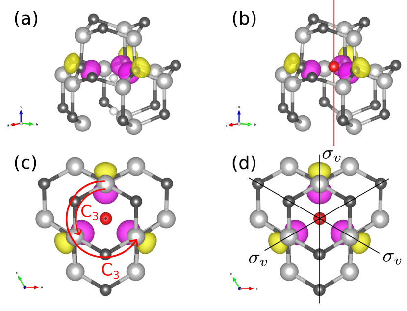
For defects in solids, the point group is determined by the crystal structure, and the symmetry of the orbitals can be described by characters and IRs. Figure 1 shows a divacancy defect in silicon carbide with the point group as an example. Comparing with the character table for , Table 4 in Appendix C, one sees that the orbital has the IR .
When defects are simulated with DFT, one obtains (one-electron) orbital wave functions and corresponding eigenvalues . Optical transitions, where an electron moves from an initial state with orbital i to a final state with orbital f, has an associated transition dipole moment (TDM) , which is expressed as:
| (1) |
where e is the electron charge and is the position operator. Selection rules can be formulated with group theory [32]. For TDM the following applies: for optical transitions to be allowed the representation of the TDM must contain the identity representation, where
| (2) |
with being the direct product, and is the IR of the polarization direction of the light, corresponding to the linear functions in the character tables.
3 Methodology
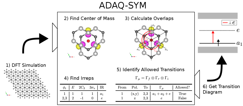
Figure 2 shows the symmetry analysis process of ADAQ-SYM. Here, we describe the steps in detail.
First, we perform a DFT simulation on a defect in a semiconductor host material. This produces a relaxed crystal structure and a set of orbital wave functions and their corresponding eigenvalues. These are the main inputs for ADAQ-SYM. The electron orbitals associated with defects are localized around the defect, and the inverse participation ratio (IPR) is a good measure of how localized an orbital is [33, 34, 35]. The discreet evaluation of IPR is
| (3) |
and can be used to identify defect orbitals in the band gap, since they have much higher IPR than the bulk orbitals. There are also defect orbitals in the bands which are hybridized with the delocalized orbitals, their IPR are lower than the ones in the band gap, but still higher than the other orbitals in the bands. We employ IPR as a tool for selecting the orbitals to be analyzed, and this method can also identify defect orbitals in the bands by spotting outliers. After the careful selection of ab initio data and inputs, ADAQ-SYM is able to perform the symmetry analysis.
Second, the ”center of mass” of the each orbital is calculated according to
| (4) |
These centers are used as the fixed points for the symmetry transformations. Orbitals are considered degenerate if the difference in their eigenvalues are less than a threshold. When calculating for degenerate orbitals, they are considered together and the average center is used.
This method does not consider periodic boundary conditions and necessitates the defect be in the middle of the unit cell. To mitigate skew of the center of mass, the wave function is sampled in real space, and points with moduli under a certain percentage of the maximum are set to zero according to
| (5) |
Third, the point group and symmetry transformations of the crystal structure is found via existing codes. Each symmetry transformation has an operator . To get characters, the overlap of an orbital wave function and its symmetry transformed counterpart, the symmetry operator expectation value (SOEV), is calculated
| (6) |
for each orbital and symmetry transformation. The wave function is expanded in a plane wave basis set, with G-vectors within the energy cutoff radius. Therefore, Eq. 6 can be rewritten to be evaluated by summing over these G-vectors only once, the plane wave expansion is also truncated by reducing the cutoff radius when reading the wave function and renormalizing [36].
Fourth, the character of a conjugacy class is taken to be the mean of the overlaps of operators within that class, and the overlaps of degenerate orbitals are added. To find the representation of a set of characters, the row of characters is projected on each IR, resulting in how many of each IR the representation contains. Consider an IR , where is a vector with the characters of times their order. For example, for the vector for is . Let be the vector with a row of characters and be the order of the point group, then is the number of times the IR occurs which is calculated as follows
| (7) |
For degenerate states the found representation should be an IR with dimension equal to the degeneracy, e.g. double degenerate orbital should have a two-dimensional state. If an IR is not found, the overlap calculation is rerun with the center of another orbital as the fixed point. The CSM for the IRs of molecular orbitals [28] is used for the defect orbitals and calculated with
| (8) |
which produces a number between 0 and 100. means that the orbital is completely consistent with IR , and means that the orbital is completely inconsistent with the IR .
Fifth, to calculate the IR of the TDM and find the allowed transitions, the characters of the TDM is calculated by taking the Hadamard (element-wise) product of the character vectors of each ’factor’
| (9) |
and Eq. 7 is used to calculate . The representation of the resulting character vector is found in the same way as the IR of the orbital was found. As an example, consider the group with the three IRs , and . If some TDM in this group has the character vector calculating the representation would look like:
| (10) |
Since contains , the transition is allowed. The software contains a function to convert a representation array of the above format to a string such as .
Finally, the information produced by ADAQ-SYM is entered into a script to produce an energy level diagram which shows the position in the band gap, orbital occupation, IR and allowed transitions.
4 Computational Details
The DFT simulations are executed with VASP [37, 38], using the projector augmented-wave method [39, 40]. We apply the periodic boundary conditions, and the defects in the adjacent supercells cause a degree of self-interaction. To limit this, the supercell needs to be sufficiently large. In our case supercells containing more than 500 atoms are used. The defects are simulated with two different exchange-correlation functionals, the semi-local functional by Perdew, Burke and Ernzerhof (PBE) [41], and the hybrid functional by Heyd, Scuseria, and Ernzerhof (HSE06) [42, 43]. The PBE simulations are presented in the supplementary material, and the HSE simulations are presented in section 5. These simulations only include the gamma point, run with a plane-wave cutoff energy of 600 eV, with the energy convergence parameters eV and eV for the electronic and ionic relaxations, respectively. The simulations are done without symmetry constraints so symmetry breaking due to the Jahn-Teller effect can occur when relaxing the crystal structure. Excited states are simulated by constraining the electron occupation [44]. For cases where an orbital in the valance band is excited to a state in the band gap the setting LDIAG=.FALSE. is used.
5 Results
To illustrate the capability of our method, we apply ADAQ-SYM to several defects in two different host materials, diamond and 4H-SiC, and analyze the symmetry properties for the defects orbitals. The symmetry analysis provides a coherent picture of the known defects, finds the allowed optical transitions between defect orbitals, and, specifically, explains the different ZPL polarization of the hk and kh divacancies in 4H-SiC. The following results are from HSE simulations, see the supplementary materials for results in PBE, as well as experimental comparisons of band gaps and ZPL energies.
5.1 Diamond Defects
We first analyze the symmetry of the ground state of NV-, SiV0 and SiV- centers. These defects were simulated in a cubic (4a,4a,4a) supercell containing 512 atoms, where Å.
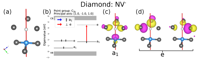
5.1.1 Negatively Charged NV Center
Figure 3 shows the ground state crystal structure and electronic structure of the NV- center in diamond. Figure 3 (b) is the generated output from ADAQ-SYM, for each orbital in the band gap. It shows the eigenvalue, occupation and IR, as well as the allowed transitions for each polarization. In this case, the found IRs are in accordance with previous work [45], and only one allowed transition is found, where the light is polarized perpendicular () to the principal axis. This selection rule has been experimentally confirmed [19].
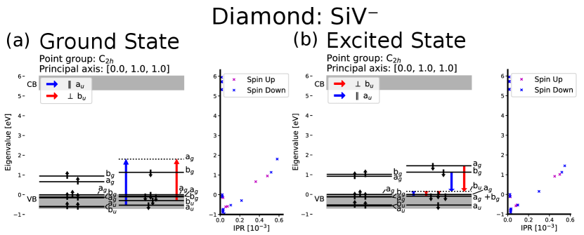
5.1.2 Silicon Vacancy Center
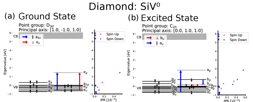
Figures 4 and 5 show the electronic structure of the neutral and negatively charged silicon vacancy center in diamond, and the IPR for 30 KS-orbitals around the band gap. Our DFT calculations show that most orbitals in the VB are delocalized and have a low IPR. However, some orbitals have larger IPRs meaning that they are more localized and indicating that they are defect states. These defect states in the VB are ungerade (u), meaning anti-symmetric with respect to inversion. Both the charge states considered in this work have point groups with inversion symmetry which only allow optical transitions between orbitals of different symmetry with respect to inversion. To populate an orbital that is gerade (g), that is symmetric with respect to inversion, an electron from an u-state must be excited. When some orbitals in the valance band are taken into account, ADAQ-SYM finds two allowed transitions from localized defect states lower in the valance band to an empty state in the band gap, while transitions from the delocalized orbitals at the top of the valance band is forbidden. Both charge states has an empty orbital in the band gap in the excited state. For both and the localized state in the VB moves to the band gap in the excited state calculation, allowing for transitions from the other band gap states. These selection rules for the SiV defects are in agreement with previous calculations [46, 47].
5.2 Silicon Carbide
In this subsection, we carry out the symmetry analysis of defects in 4H-SiC with ADAQ-SYM, in both the ground state and the lowest excited state. The IR of each KS-orbital in the band gap and the allowed polarization of light for both absorption and emission is shown in the figures below. 4H-SiC consists of alternating hexagonal () and quasi-cubic () layers, resulting in different defect configurations for the same stoichiometry. The defects were simulated in a hexagonal (6a,6a,2c) supercell containing 576 atoms, where Å and Å. For 4H-SiC, ”in-plane” refers to the plane perpendicular to the c-axis.
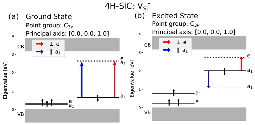
5.2.1 Negatively Charged Silicon Vacancy
We simulated the ground and excited state of the negatively charged silicon vacancy in the site. Figure 6 (a) shows two allowed transitions with different polarization, where the parallel polarized transition has slightly lower energy than the perpendicular, this corresponds well to the V1 and V1’ absorption lines [48] associated with the silicon vacancy in the h site [49]. Figure 6 (b) shows that the transition back to the ground state emits light polarized parallel to the c-axis, in agreement with previous calculations and measurements regarding the polarization of the V1 ZPL [50, 8].
5.2.2 High Symmetry Divacancy
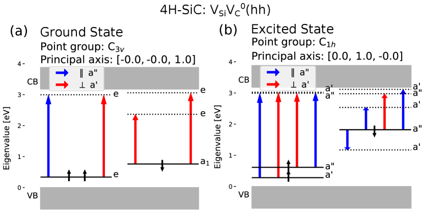
Figure 7 shows the ground and excited state of the configuration of the divacancy, and the allowed transitions. In the excited state, one electron occupies what was previously an empty degenerate state and causes an Jahn-Teller effect. Because of this, the point group symmetry is reduced from to and degenerate states split when the system is relaxed in our simulations. This also changes the principal axis from being parallel to the c-axis to being perpendicular to it, that is the principal axis now lies in-plane. The selection rule tells us that absorption (to the lowest excited state) happens only for light polarized perpendicular to the c-axis, and the transition from the excited state emits light polarized parallel to the in-plane principal axis, thus also perpendicular to the c-axis. This polarization behavior corresponds well to previous calculations and measurements [18, 51]. The divacancy is basically identical to the divacancy with respect to symmetry.
5.2.3 Distinguishing Low Symmetry Divacancies
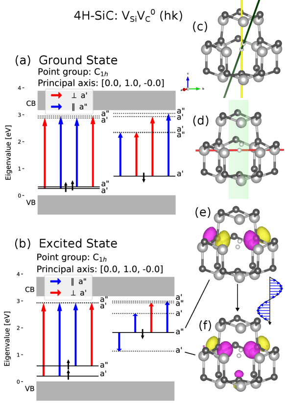
The two low symmetry divacancy configurations and exhibit different behavior regarding the polarization of the ZPL [18, 51]. Examining the symmetry of the orbitals and applying selection rules regarding the TDM allows us to distinguish between these configurations. For both of these low symmetry configurations, the only symmetry transformation in the ground state is a reflection in a plane where the principal axis lies in-plane. Figure 8 shows crystal- and electronic structure information of the divacancy. From panel (b) one sees that the relaxation to the ground state only emits light polarized parallel to the in-plane principal axis. Figure 9 shows crystal- and electronic structure information of the divacancy. In the excited state the crystal is slightly symmetry broken from to , this is barely visible in panel (c). However, it is clear from the symmetry analysis of the relaxed ions. This symmetry breaking was not found in the PBE calculations and only appeared when the crystal structure for the excited state was relaxed using the HSE functional. Thus no optical transition is forbidden by the selection rules. Further analysis of the orbitals of the excited state in the point group is presented in the supplementary material, this analysis indicates the transition may be between two symmetric orbitals where the allowed polarization is perpendicular to an in-plane axis. In either case, excited state is C1h or C1, gives the same selection rules that are consistent with experimental results.

6 Discussion
From the symmetry analysis by ADAQ-SYM, one can attribute the differing polarization behavior of the and configurations to the symmetry of the lowest excited state, anti-symmetric and asymmetric (possibly symmetric) respectively. Due to the principal axis laying in-plane, different defect orientations will also emit out-of-plane with different polarization. Thus, it may be possible to experimentally determine the orientation of individual defects measuring the in-plane polarization angle of the PL detected along the c-axis, in an experiment similar to Alegre et al. [19]. In such an experiment, the divacancy will exhibit a luminescence intensity maxima when the polarization is parallel to the principal axis, and a minima when the polarization in perpendicular. The opposite would be true for the divacancy, and the two configurations could be distinguished by the approximately 30 meV difference in ZPL [18], or by the 30 degree polarization differences between the respective maxima, see supplementary material for polar plots of this polarization dependence.
Having a loose tolerance parameter for the AFLOW-SYM crystal symmetry finder can be useful in ambiguous cases since ADAQ-SYM will then run for a larger set of symmetry operators, which gives an overview and can provide insight to what extent the orbitals are asymmetric with regards to each operator. It is also recommended to do this when multiple gradual distortions of the same defect are examined. The initial PBE excited state calculation of the silicon vacancy in 4H-SiC seemed to show a case of the pseudo Jahn-Teller effect where the symmetry was reduced and the degenerate states split despite not being partially occupied in either spin channel. Upon running a simulation with more accurate tolerance parameters the point group remained and the splitting reduced to less than the threshold of 10 meV. This effect did not appear in the HSE simulation. For cases where the occupied state is very close to empty states convergence becomes more important and looser high-throughput simulations may exaggerate these effects. To resolve this one can either run more accurate calculations, or have a higher degeneracy tolerance parameter which will cause more states to be grouped together as degenerate.
7 Conclusion
We have presented a method of determining the symmetry of defect orbitals, and implemented this method in the software ADAQ-SYM. The implementation calculates the characters and irreducible representations of defect orbitals, the continuous symmetry measure is also calculated to get a numerical measure of how close the orbitals are described by the irreducible representations. Finally, ADAQ-SYM applies selection rules to the optical transitions between the orbitals. The tool is applicable to efficient analysis of defects. We have applied the tool to a variety of known defects with different point groups and host materials, and it reliably reproduces their symmetry properties. In addition to the reproduction of prior results, we find that the polarization of the allowed transition for is parallel to an in-plane axis, and while exhibits slightly broken symmetry, the polarization is perpendicular to an in-plane axis. A method to determine the orientation of individual and divacancies is also proposed. In summary, ADAQ-SYM is an automated defect symmetry analysis tool which is useful for both manual and high-throughput calculations.
Software Availability
For availability of ADAQ-SYM and instructions, see https://httk.org/adaq/.
Author contributions
William Stenlund: Conceptualization, Investigation, Methodology, Software, Validation, Visualization, Writing - original draft. Joel Davidsson: Conceptualization, Methodology, Supervision, Writing - review & editing. Rickard Armiento: Conceptualization, Supervision, Writing - review & editing. Viktor Ivády: Conceptualization, Methodology, Supervision, Writing - review & editing. Igor A. Abrikosov: Conceptualization, Supervision, Writing - review & editing.
Declaration of Competing Interest
The authors declare that they have no known competing financial interests or personal relationships that could have appeared to influence the work reported in this paper.
Acknowledgements
This work was partially supported by the Knut and Alice Wallenberg Foundation through the Wallenberg Centre for Quantum Technology (WACQT). We acknowledge support from the Knut and Alice Wallenberg Foundation (Grant No. 2018.0071). Support from the Swedish Government Strategic Research Area Swedish e-science Research Centre (SeRC) and the Swedish Government Strategic Research Area in Materials Science on Functional Materials at Linköping University (Faculty Grant SFO-Mat-LiU No. 2009 00971) are gratefully acknowledged. JD and RA acknowledge support from the Swedish Research Council (VR) Grant No. 2022-00276 and 2020-05402, respectively. The computations were enabled by resources provided by the National Academic Infrastructure for Supercomputing in Sweden (NAISS) and the Swedish National Infrastructure for Computing (SNIC) at NSC, partially funded by the Swedish Research Council through grant agreements no. 2022-06725 and no. 2018-05973. This research was supported by the National Research, Development, and Innovation Office of Hungary within the Quantum Information National Laboratory of Hungary (Grant No. 2022-2.1.1-NL-2022-00004) and within grant FK 145395.
Appendix A Implementation
ADAQ-SYM is written in python using functional programming. Table 1 provides an overview of the principal functions, and Table 2 shows the settings ADAQ-SYM uses. To run the code, the user needs to provide three files from a VASP simulation; POSCAR or CONTCAR, the crystal structure; WAVECAR, wave function; EIGENVAL, eigenvalues and occupation of the bands. To select which bands get analyzed, either use the IPR threshold or select the bands manually. For now, the code only works for defects simulated at the Gamma-point.
| Function name | Output |
|---|---|
| get_symmetry_operators() | transformation matrices |
| get_point_group() | point group |
| find_average_position() | centers |
| get_overlaps_of_bands() | overlaps |
| get_energy_and_band_degen() | degeneracy grouping |
| get_character() | characters |
| get_rep() | representation |
| get_allowed_transitions() | transitions |
| plot_levels() | diagram |
| Name | Description | Default |
| aflow_tolerance | AFLOW-SYM tolerance parameter | tight |
| degeneracy_tolerance | Max energy differance between degenerate bands | 0.01 |
| IR_tolerance | Maximun deviation of from integer | 0.05 |
| Gvec_reduction | Cutoff energy of plane wave is multiplied by this | 0.15 |
| realgrid_mult | Increases grid density when calculating 4 | 4 |
| percent_cutoff | Percentage in Eq. 5 | 0.40 |
The functions get_point_group() and get_symmetry_operators() call AFLOW-SYM [21] to find the point group and symmetry operators of the input crystal structure, the symmetry operators are then sorted by their conjugacy class and arranged in the order the classes appear in the character table. These functions use the aflow_tolerance setting which determine tolerance for asymmetry AFLOW-SYM uses, values may be ”tight” or ”loose”. The point group is used to load the right character table from text files by Gernot Katzer [52]. The vaspwfc module in the VaspBandUnfolding package [53] is used for reading the WAVECAR file and working with the plane wave expansion of the wave function, and it also serves as the basis of the IPR calculations.
The function find_average_position_general() calculates the ”center of mass” of each of the considered bands using Eq. 4 and 5, where the cutoff percentage is read from the percent_cutoff setting. The wave function is sampled in a real space grid where the realgrid_mult setting makes the grid denser. The function get_overlaps_of_bands() loops through all considered orbitals and all symmetry operators and calculates the overlap, how Eq. 6 is computed is described in more detail in [36] and Numpy [54] is used to accelerate the evaluation. The evaluation time of the overlap calculation scales linearly with the number of G-vectors in the plane wave expansion. To speed up the software the series is truncated by multiplying the cutoff energy by the factor Gvec_reduction. The cutoff energy corresponds to a radius in k-space and only G-vectors within the radius are used, so halving the cutoff energy gives roughly one eighth as many G-vectors. Truncating the series produces some error in the overlap, this error is relatively small for Gvec_reduction larger than 0.1 [36], the symmetry does not depend strongly on the high frequency components of the plane wave expansion. Note that the overlap calculation will produce a complex number. The function get_energy_and_band_degen() reads the EIGENVAL file and groups the considered bands by degeneracy. Two bands are considered degenerate if the difference in eigenvalue is less than degeneracy_tolerance. This function also outputs the eigenvalue and occupation of the considered bands.
The function get_character() takes the overlaps and the bands grouped by degeneracy and first adds the overlaps of degenerate bands for each symmetry operator, then the overlaps within each conjugacy class is averaged to produce the character. At this point, the character is complex valued but this is resolved with the following function. The function get_rep() takes a set of characters and computes Eq. 7 for all IRs of a point group, since the overlaps are in general complex will also be a complex number. Doing this for a truly symmetric orbital will produce a complex number with a small imaginary component and a real component close to an integer. For a set of characters to be said to transform as IR , the imaginary component must be smaller than IR_tolerance and the real component must be within IR_tolerance of a non-zero integer. For example with a tolerance of 0.05, characters producing will be interpreted as transforming as IR , while characters producing or will not. The same procedure is used when the CSM is calculated, since Eq. 8 uses . The function get_allowed_transitions() calculates Eq. 9 for each occupied state i, each non-full state f and each linear function r. The representation is found with get_rep() and if the trivial representation is contained, the transition is marked as allowed. The function plot_levels() uses Matplotlib [55] to create energy level diagrams of the considered states with the occupation and IR drawn, and all allowed transitions represented by arrows between the bands. The color of the arrow differs on the polarization of the transition. The levels of the VB and CB are determined by the eigenvalues of the delocalized orbitals above and below the localized orbitals. For cases where defect orbitals are found in the VB or CB, e.g. when all localized orbitals are not adjacent in terms of eigenvalue, it is recommended set the VB and CB eigenvalues manually in plotting script, look for the eigenvalues of the delocalized orbitals at the VB and CB edges.
Appendix B Troubleshooting
The following summarizes our recommendations when running the tool:
If no IR is found and several bands are close, increase degeneracy tolerance which will cause more states to be grouped together as degenerate. This may be preferential since actually degenerate orbitals split apart will not be assigned any IR, while accidentally degenerate orbitals grouped together as degenerate will assigned an IR which is the sum each orbitals IR, such as , which makes it clear that the orbitals are accidentally degenerate.
If no IR is found, check that the centers of mass are close to your defect. If not, recalculate the centers with higher grid density, setting realgrid_mult 6 or 8. There is also an automated fallback where the atomic position of any unique atomic species will be used.
If the crystal symmetry is unclear or you think it should be higher, increase AFLOWs tolerance. This way, the overlaps will be calculated for a larger set of symmetry operators.Then, check the overlaps manually, and look for subsets where the characters are close to integers, any such subset should be a point group which is a subset of the larger group.
Appendix C Character tables
The character tables used in this paper are presented here. The tables include the linear and quadratic basis functions for the respective point groups.
| E | Linear | Quadratic | ||
|---|---|---|---|---|
| 1 | 1 | x,y | ||
| 1 | -1 | z |
| E | Linear | Quadratic | |||
|---|---|---|---|---|---|
| 1 | 1 | 1 | z | ||
| 1 | 1 | -1 | |||
| 2 | -1 | 0 | (x,y) |
| E | i | Linear | Quadratic | |||
|---|---|---|---|---|---|---|
| 1 | 1 | 1 | 1 | |||
| 1 | -1 | 1 | -1 | |||
| 1 | 1 | -1 | -1 | z | ||
| 1 | -1 | -1 | 1 | x,y |
| E | i | Linear | Quadratic | |||||
|---|---|---|---|---|---|---|---|---|
| 1 | 1 | 1 | 1 | 1 | 1 | |||
| 1 | 1 | -1 | 1 | 1 | -1 | |||
| 2 | -1 | 0 | 2 | -1 | 0 | |||
| 1 | 1 | 1 | -1 | -1 | -1 | |||
| 1 | 1 | -1 | -1 | -1 | 1 | z | ||
| 2 | -1 | 0 | -2 | 1 | 0 | (x,y) |
References
- Koehl et al. [2011] W. F. Koehl, B. B. Buckley, F. J. Heremans, G. Calusine, D. D. Awschalom, Room temperature coherent control of defect spin qubits in silicon carbide, Nature 479 (2011) 84–87. URL: https://doi.org/10.1038/nature10562. doi:10.1038/nature10562.
- Pezzagna and Meijer [2021] S. Pezzagna, J. Meijer, Quantum computer based on color centers in diamond, Applied Physics Reviews 8 (2021) 011308. URL: https://doi.org/10.1063/5.0007444. doi:10.1063/5.0007444. arXiv:https://doi.org/10.1063/5.0007444.
- Kalhor et al. [2021] F. Kalhor, L.-P. Yang, L. Bauer, Z. Jacob, Quantum sensing of photonic spin density using a single spin qubit, Phys. Rev. Res. 3 (2021) 043007. URL: https://link.aps.org/doi/10.1103/PhysRevResearch.3.043007. doi:10.1103/PhysRevResearch.3.043007.
- Mzyk et al. [2022] A. Mzyk, A. Sigaeva, R. Schirhagl, Relaxometry with nitrogen vacancy (nv) centers in diamond, Accounts of Chemical Research 55 (2022) 3572–3580. URL: https://doi.org/10.1021/acs.accounts.2c00520. doi:10.1021/acs.accounts.2c00520.
- Berhane et al. [2017] A. M. Berhane, K.-Y. Jeong, Z. Bodrog, S. Fiedler, T. Schröder, N. V. Triviño, T. Palacios, A. Gali, M. Toth, D. Englund, I. Aharonovich, Bright room-temperature single-photon emission from defects in gallium nitride, Advanced Materials 29 (2017) 1605092. URL: https://onlinelibrary.wiley.com/doi/abs/10.1002/adma.201605092. doi:https://doi.org/10.1002/adma.201605092. arXiv:https://onlinelibrary.wiley.com/doi/pdf/10.1002/adma.201605092.
- Zhang et al. [2020] G. Zhang, Y. Cheng, J.-P. Chou, A. Gali, Material platforms for defect qubits and single-photon emitters, Applied Physics Reviews 7 (2020). URL: https://doi.org/10.1063/5.0006075. doi:10.1063/5.0006075. arXiv:https://pubs.aip.org/aip/apr/article-pdf/doi/10.1063/5.0006075/14576561/031308_1_online.pdf, 031308.
- Castelletto and Boretti [2020] S. Castelletto, A. Boretti, Silicon carbide color centers for quantum applications, Journal of Physics: Photonics 2 (2020) 022001. URL: https://dx.doi.org/10.1088/2515-7647/ab77a2. doi:10.1088/2515-7647/ab77a2.
- Davidsson et al. [2022] J. Davidsson, R. Babar, D. Shafizadeh, I. G. Ivanov, V. Ivády, R. Armiento, I. A. Abrikosov, Exhaustive characterization of modified si vacancies in 4h-sic, Nanophotonics 11 (2022) 4565–4580. URL: https://doi.org/10.1515/nanoph-2022-0400. doi:doi:10.1515/nanoph-2022-0400.
- Freysoldt et al. [2014] C. Freysoldt, B. Grabowski, T. Hickel, J. Neugebauer, G. Kresse, A. Janotti, C. G. Van de Walle, First-principles calculations for point defects in solids, Rev. Mod. Phys. 86 (2014) 253–305. URL: https://link.aps.org/doi/10.1103/RevModPhys.86.253. doi:10.1103/RevModPhys.86.253.
- Ivády et al. [2018] V. Ivády, I. A. Abrikosov, A. Gali, First principles calculation of spin-related quantities for point defect qubit research, npj Computational Materials 4 (2018) 76. URL: https://doi.org/10.1038/s41524-018-0132-5. doi:10.1038/s41524-018-0132-5.
- Dreyer et al. [2018] C. E. Dreyer, A. Alkauskas, J. L. Lyons, A. Janotti, C. G. Van de Walle, First-principles calculations of point defects for quantum technologies, Annual Review of Materials Research 48 (2018) 1–26. URL: https://doi.org/10.1146/annurev-matsci-070317-124453. doi:10.1146/annurev-matsci-070317-124453.
- Sluydts et al. [2017] M. Sluydts, M. Pieters, J. Vanhellemont, V. Van Speybroeck, S. Cottenier, High-throughput screening of extrinsic point defect properties in si and ge: Database and applications, Chemistry of Materials 29 (2017) 975–984. URL: https://doi.org/10.1021/acs.chemmater.6b03368. doi:10.1021/acs.chemmater.6b03368.
- Broberg et al. [2018] D. Broberg, B. Medasani, N. E. Zimmermann, G. Yu, A. Canning, M. Haranczyk, M. Asta, G. Hautier, Pycdt: A python toolkit for modeling point defects in semiconductors and insulators, Computer Physics Communications 226 (2018) 165–179. URL: https://www.sciencedirect.com/science/article/pii/S0010465518300079. doi:https://doi.org/10.1016/j.cpc.2018.01.004.
- Davidsson et al. [2021] J. Davidsson, V. Ivády, R. Armiento, I. A. Abrikosov, Adaq: Automatic workflows for magneto-optical properties of point defects in semiconductors, Computer Physics Communications 269 (2021) 108091. URL: https://www.sciencedirect.com/science/article/pii/S0010465521002034. doi:https://doi.org/10.1016/j.cpc.2021.108091.
- Bertoldo et al. [2022] F. Bertoldo, S. Ali, S. Manti, K. S. Thygesen, Quantum point defects in 2d materials - the qpod database, npj Computational Materials 8 (2022) 56. URL: https://doi.org/10.1038/s41524-022-00730-w. doi:10.1038/s41524-022-00730-w.
- Bulancea-Lindvall et al. [2023] O. Bulancea-Lindvall, J. Davidsson, R. Armiento, I. A. Abrikosov, Chlorine vacancy in : An nv-like defect with telecom-wavelength emission, Phys. Rev. B 108 (2023) 224106. URL: https://link.aps.org/doi/10.1103/PhysRevB.108.224106. doi:10.1103/PhysRevB.108.224106.
- Davidsson et al. [2023] J. Davidsson, W. Stenlund, A. S. Parackal, R. Armiento, I. A. Abrikosov, Na in diamond: High spin defects revealed by the adaq high-throughput computational database, 2023. arXiv:2306.11116.
- Davidsson [2020] J. Davidsson, Theoretical polarization of zero phonon lines in point defects, Journal of Physics: Condensed Matter 32 (2020) 385502. URL: https://doi.org/10.1088/1361-648x/ab94f4. doi:10.1088/1361-648x/ab94f4.
- Alegre et al. [2007] T. P. M. Alegre, C. Santori, G. Medeiros-Ribeiro, R. G. Beausoleil, Polarization-selective excitation of nitrogen vacancy centers in diamond, Phys. Rev. B 76 (2007) 165205. URL: https://link.aps.org/doi/10.1103/PhysRevB.76.165205. doi:10.1103/PhysRevB.76.165205.
- Togo and Tanaka [2018] A. Togo, I. Tanaka, Spglib: a software library for crystal symmetry search, 2018. arXiv:1808.01590.
- Hicks et al. [2018] D. Hicks, C. Oses, E. Gossett, G. Gomez, R. H. Taylor, C. Toher, M. J. Mehl, O. Levy, S. Curtarolo, AFLOW-SYM: platform for the complete, automatic and self-consistent symmetry analysis of crystals, Acta Crystallographica Section A 74 (2018) 184–203. URL: https://doi.org/10.1107/S2053273318003066. doi:10.1107/S2053273318003066.
- Gao et al. [2021] J. Gao, Q. Wu, C. Persson, Z. Wang, Irvsp: To obtain irreducible representations of electronic states in the vasp, Computer Physics Communications 261 (2021) 107760. URL: https://www.sciencedirect.com/science/article/pii/S0010465520303805. doi:https://doi.org/10.1016/j.cpc.2020.107760.
- Iraola et al. [2022] M. Iraola, J. L. Mañes, B. Bradlyn, M. K. Horton, T. Neupert, M. G. Vergniory, S. S. Tsirkin, Irrep: Symmetry eigenvalues and irreducible representations of ab initio band structures, Computer Physics Communications 272 (2022) 108226. URL: https://www.sciencedirect.com/science/article/pii/S0010465521003386. doi:https://doi.org/10.1016/j.cpc.2021.108226.
- Liu et al. [2021] G.-B. Liu, M. Chu, Z. Zhang, Z.-M. Yu, Y. Yao, Spacegroupirep: A package for irreducible representations of space group, Computer Physics Communications 265 (2021) 107993. URL: https://www.sciencedirect.com/science/article/pii/S0010465521001053. doi:https://doi.org/10.1016/j.cpc.2021.107993.
- Matsugatani et al. [2021] A. Matsugatani, S. Ono, Y. Nomura, H. Watanabe, qeirreps: An open-source program for quantum espresso to compute irreducible representations of bloch wavefunctions, Computer Physics Communications 264 (2021) 107948. URL: https://www.sciencedirect.com/science/article/pii/S0010465521000722. doi:https://doi.org/10.1016/j.cpc.2021.107948.
- Zabrodsky et al. [1992] H. Zabrodsky, S. Peleg, D. Avnir, Continuous symmetry measures, Journal of the American Chemical Society 114 (1992) 7843–7851. URL: https://pubs.acs.org/doi/abs/10.1021/ja00046a033. doi:10.1021/ja00046a033. arXiv:https://doi.org/10.1021/ja00046a033.
- Dryzun and Avnir [2009] C. Dryzun, D. Avnir, Generalization of the continuous symmetry measure: the symmetry of vectors, matrices, operators and functions, Phys. Chem. Chem. Phys. 11 (2009) 9653–9666. URL: http://dx.doi.org/10.1039/B911179D. doi:10.1039/B911179D.
- Alemany et al. [2012] P. Alemany, D. Casanova, S. Álvarez, Continuous symmetry measures of irreducible representations: application to molecular orbitals, Phys. Chem. Chem. Phys. 14 (2012) 11816–11823. URL: http://dx.doi.org/10.1039/C2CP41506B. doi:10.1039/C2CP41506B.
- Beevers et al. [2023] C. Beevers, S. Francis, A. Roldan, Symmetry analysis of irregular objects, Journal of Mathematical Chemistry 61 (2023) 504–519. URL: https://doi.org/10.1007/s10910-022-01423-x. doi:10.1007/s10910-022-01423-x.
- Hossain et al. [2008] F. M. Hossain, M. W. Doherty, H. F. Wilson, L. C. L. Hollenberg, Ab initio electronic and optical properties of the center in diamond, Phys. Rev. Lett. 101 (2008) 226403. URL: https://link.aps.org/doi/10.1103/PhysRevLett.101.226403. doi:10.1103/PhysRevLett.101.226403.
- Herrero-Saboya et al. [2022] G. Herrero-Saboya, L. Martin-Samos, N. Richard, A. Hemeryck, Common defects in diamond lattices as instances of the general t jahn-teller effect, Phys. Rev. Mater. 6 (2022) 034601. URL: https://link.aps.org/doi/10.1103/PhysRevMaterials.6.034601. doi:10.1103/PhysRevMaterials.6.034601.
- Dresselhaus et al. [2008] M. Dresselhaus, G. Dresselhaus, A. Jorio, Group Theory: Application to the Physics of Condensed Matter, Springer Berlin Heidelberg, 2008. URL: https://www.springer.com/gp/book/9783540328971#. doi:10.1007/978-3-540-32899-5.
- Wegner [1980] F. Wegner, Inverse participation ratio in 2+ dimensions, Zeitschrift für Physik B Condensed Matter 36 (1980). URL: https://doi.org/10.1007/BF01325284. doi:10.1007/BF01325284.
- Kramer and MacKinnon [1993] B. Kramer, A. MacKinnon, Localization: theory and experiment, Reports on Progress in Physics 56 (1993) 1469. URL: https://dx.doi.org/10.1088/0034-4885/56/12/001. doi:10.1088/0034-4885/56/12/001.
- Pashartis and Rubel [2017] C. Pashartis, O. Rubel, Localization of electronic states in iii-v semiconductor alloys: A comparative study, Phys. Rev. Appl. 7 (2017) 064011. URL: https://link.aps.org/doi/10.1103/PhysRevApplied.7.064011. doi:10.1103/PhysRevApplied.7.064011.
- Stenlund [2022] W. Stenlund, Symmetry analysis of orbitals in a plane wave basis: A study on molecules and defects in solids, 2022. URL: http://urn.kb.se/resolve?urn=urn:nbn:se:liu:diva-180194.
- Kresse and Hafner [1994] G. Kresse, J. Hafner, Ab initio molecular-dynamics simulation of the liquid-metal–amorphous-semiconductor transition in germanium, Phys. Rev. B 49 (1994) 14251–14269. URL: http://link.aps.org/doi/10.1103/PhysRevB.49.14251. doi:10.1103/PhysRevB.49.14251.
- Kresse and Furthmüller [1996] G. Kresse, J. Furthmüller, Efficient iterative schemes for ab initio total-energy calculations using a plane-wave basis set, Phys. Rev. B 54 (1996) 11169–11186. URL: http://link.aps.org/doi/10.1103/PhysRevB.54.11169. doi:10.1103/PhysRevB.54.11169.
- Blöchl [1994] P. E. Blöchl, Projector augmented-wave method, Phys. Rev. B 50 (1994) 17953–17979. URL: http://link.aps.org/doi/10.1103/PhysRevB.50.17953. doi:10.1103/PhysRevB.50.17953.
- Kresse and Joubert [1999] G. Kresse, D. Joubert, From ultrasoft pseudopotentials to the projector augmented-wave method, Phys. Rev. B 59 (1999) 1758–1775. URL: http://link.aps.org/doi/10.1103/PhysRevB.59.1758. doi:10.1103/PhysRevB.59.1758.
- Perdew et al. [1996] J. P. Perdew, K. Burke, M. Ernzerhof, Generalized gradient approximation made simple, Phys. Rev. Lett. 77 (1996) 3865–3868. URL: http://link.aps.org/doi/10.1103/PhysRevLett.77.3865. doi:10.1103/PhysRevLett.77.3865.
- Heyd et al. [2003] J. Heyd, G. E. Scuseria, M. Ernzerhof, Hybrid functionals based on a screened coulomb potential, The Journal of Chemical Physics 118 (2003) 8207–8215. URL: https://doi.org/10.1063/1.1564060. doi:10.1063/1.1564060. arXiv:https://doi.org/10.1063/1.1564060.
- Heyd et al. [2006] J. Heyd, G. E. Scuseria, M. Ernzerhof, Erratum: “hybrid functionals based on a screened coulomb potential” [j. chem. phys. 118, 8207 (2003)], The Journal of Chemical Physics 124 (2006) 219906. URL: https://doi.org/10.1063/1.2204597. doi:10.1063/1.2204597. arXiv:https://doi.org/10.1063/1.2204597.
- Gali et al. [2009] A. Gali, E. Janzén, P. Deák, G. Kresse, E. Kaxiras, Theory of spin-conserving excitation of the center in diamond, Phys. Rev. Lett. 103 (2009) 186404. URL: https://link.aps.org/doi/10.1103/PhysRevLett.103.186404. doi:10.1103/PhysRevLett.103.186404.
- Doherty et al. [2011] M. W. Doherty, N. B. Manson, P. Delaney, L. C. L. Hollenberg, The negatively charged nitrogen-vacancy centre in diamond: the electronic solution, New Journal of Physics 13 (2011) 025019. URL: https://dx.doi.org/10.1088/1367-2630/13/2/025019. doi:10.1088/1367-2630/13/2/025019.
- Thiering and Gali [2018] G. Thiering, A. Gali, Ab initio magneto-optical spectrum of group-iv vacancy color centers in diamond, Phys. Rev. X 8 (2018) 021063. URL: https://link.aps.org/doi/10.1103/PhysRevX.8.021063. doi:10.1103/PhysRevX.8.021063.
- Xiong et al. [2023] Y. Xiong, M. Mathew, S. M. Griffin, A. Sipahigil, G. Hautier, Midgap state requirements for optically active quantum defects, 2023. arXiv:2302.10767.
- Janzén et al. [2009] E. Janzén, A. Gali, P. Carlsson, A. Gällström, B. Magnusson, N. Son, The silicon vacancy in sic, Physica B: Condensed Matter 404 (2009) 4354–4358. URL: https://www.sciencedirect.com/science/article/pii/S0921452609010862. doi:https://doi.org/10.1016/j.physb.2009.09.023.
- Ivády et al. [2017] V. Ivády, J. Davidsson, N. T. Son, T. Ohshima, I. A. Abrikosov, A. Gali, Identification of si-vacancy related room-temperature qubits in silicon carbide, Phys. Rev. B 96 (2017) 161114(R). URL: https://link.aps.org/doi/10.1103/PhysRevB.96.161114. doi:10.1103/PhysRevB.96.161114.
- Gali [2012] A. Gali, Excitation properties of silicon vacancy in silicon carbide, in: Silicon Carbide and Related Materials 2011, volume 717 of Materials Science Forum, Trans Tech Publications Ltd, 2012, pp. 255–258. doi:10.4028/www.scientific.net/MSF.717-720.255.
- Gällström [2015] A. Gällström, Optical Characterization of Deep Level Defects in SiC, Ph.D. thesis, Linköping University, Semiconductor Materials, The Institute of Technology, 2015.
- Katzer [????] G. Katzer, Character tables for point groups used in chemistry, ???? URL: http://www.gernot-katzers-spice-pages.com/character_tables/, accessed: 2023-01-27.
- Zheng [????] Q. Zheng, Qijingzheng/vaspbandunfolding, ???? URL: https://github.com/QijingZheng/VaspBandUnfolding, accessed: 2022.
- Harris et al. [2020] C. R. Harris, K. J. Millman, S. J. van der Walt, R. Gommers, P. Virtanen, D. Cournapeau, E. Wieser, J. Taylor, S. Berg, N. J. Smith, R. Kern, M. Picus, S. Hoyer, M. H. van Kerkwijk, M. Brett, A. Haldane, J. Fernández del Río, M. Wiebe, P. Peterson, P. Gérard-Marchant, K. Sheppard, T. Reddy, W. Weckesser, H. Abbasi, C. Gohlke, T. E. Oliphant, Array programming with NumPy, Nature 585 (2020) 357–362. doi:10.1038/s41586-020-2649-2.
- Hunter [2007] J. D. Hunter, Matplotlib: A 2d graphics environment, Computing in Science & Engineering 9 (2007) 90–95. doi:10.1109/MCSE.2007.55.