This paper was converted on www.awesomepapers.org from LaTeX by an anonymous user.
Want to know more? Visit the Converter page.

\floatevery

algorithm

Adjoint sharding for very long context training of state space models

Xingzi Xu1,2\ {}^{1,2} &Amir Tavanaei1\ {}^{1} &Kavosh Asadi1\ {}^{1} &Karim Bouyarmane1\ {}^{1} \AND
1 Amazon
Seattle, WA 98109, USA
{xingzixu,atavanae,kavasadi,bouykari}@amazon.com &
2  Duke University
Durham, NC 27708, USA
xingzi.xu@duke.edu
Work done during internship at Amazon.
Abstract

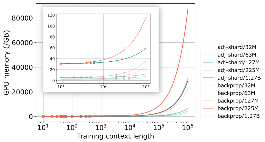
Despite very fast progress, efficiently training large language models (LLMs) in very long contexts remains challenging. Existing methods fall back to training LLMs with short contexts (a maximum of a few thousands tokens in training) and use inference time techniques when evaluating on long contexts (above 1M tokens context window at inference). As opposed to long-context-inference, training on very long context input prompts is quickly limited by GPU memory availability and by the prohibitively long training times it requires on state-of-the-art hardware. Meanwhile, many real-life applications require not only inference but also training/fine-tuning with long context on specific tasks. Such applications include, for example, augmenting the context with various sources of raw reference information for fact extraction, fact summarization, or fact reconciliation tasks. We propose adjoint sharding, a novel technique that comprises sharding gradient calculation during training to reduce memory requirements by orders of magnitude, making training on very long context computationally tractable. Adjoint sharding is based on the adjoint method and computes equivalent gradients to backpropagation. We also propose truncated adjoint sharding to speed up the algorithm while maintaining performance. We provide a distributed version, and a paralleled version of adjoint sharding to further speed up training. Empirical results show the proposed adjoint sharding algorithm reduces memory usage by up to 3X with a 1.27B parameter large language model on 1M context length training. This allows to increase the maximum context length during training or fine-tuning of a 1.27B parameter model from 35K tokens to above 100K tokens on a training infrastructure composed of five AWS P4 instances. 333Additional material for this paper can be found at: https://adjoint-sharding.github.io.

Refer to caption
Figure 1: Compared to backpropagation (red lines), adjoint sharding (blue lines) significantly reduces memory requirements at training. Showing memory cost to train 32M32\mathrm{M}, 63M63\mathrm{M}, 127M127\mathrm{M}, 225M225\mathrm{M}, and 1.27B1.27\mathrm{B} parameter State Space Model (SSM) with batch size 22 and Adam optimizer on one GPU.

1 Introduction

Foundation models are a new paradigm in artificial intelligence research focused on building large, general-purpose models that adapt to different tasks [44, 40, 7, 51]. Extensive training on large datasets equips foundation models with broad capabilities, which are then fine-tuned on smaller datasets for specific applications. Foundation models commonly employ the transformer architecture [60]. Despite the immense success, training transformer-based models requires memory growing quadratically with the context length LL, limiting their applications on long context tasks [36]. Researchers developed various techniques to conquer this problem, ranging from inference time context window expansion [19, 18], IO-aware algorithms [16, 13, 55], and various linearly scaling language model architectures [23, 15, 49, 6]. On another note, distributed learning enables training large models with a big number of GPUs, and efficient training methods like activation checkpointing, model/gradient sharding, and mixed-precision computing have further reduced the memory requirement of training a large model [61, 69, 53, 41, 30]. However, current methodologies are entirely based on backpropagation and compute the gradient as a whole, inevitably requiring a memory growing rapidly with model size and context length [12]. Current sharding methods ignore the activations and only consider the model weights and optimizer states, constituting only a small fraction of the total memory cost [56]. Activation checkpointing is among the limited techniques that consider activation values. Activation checkpointing offloads necessary intermediate states to the CPU and recompute them on the fly, trading compute time for memory reduction [56, 52]. The substantial time required for offloading to the CPU hinders the effectiveness of activation checkpointing.

We propose adjoint sharding to dissemble gradient computation of residual and/or recurrent based models to achieve orders of magnitude lower memory usage during training.

Refer to caption
Figure 2: Adjoint sharding dissembles large models’ gradient computations along the sequence dimension tt and the layer dimension kk. When evaluating the gradient at time tt, we perform tt vector-Jacobian products along the adjoint dimension ii for every layer indices kk.

Adjoint method

The adjoint sharding method is based on the adjoint method for recurrent models [8, 32]. Given an optimization problem of a parametric recurrent forward process, the adjoint method is concerned with computations of the gradients regarding the process’s parameters. Backpropagation saves intermediate states to calculate gradients, whereas the adjoint method relies on a backward adjoint process to compute gradients. The adjoint method is a constant-memory optimization technique for dynamical systems [9, 66]. In this paper, we are only concerned with the adjoint method for recurrent relations.

Vector-Jacobian product

Adjoint sharding dissembles the gradient computation of a large language model (LLM) into independent vector-Jacobian product (VJP) computations. By left-multiplying the Jacobian with a vector, it becomes unnecessary to compute the expensive Jacobian. Modern VJPs are as fast as a forward function call of the model, and can be thousands of times faster than Jacobian computations [2]. We speed up adjoint sharding by employing the VJPs.

Truncated adjoint sharding

Sharding the gradient computation allows us to prioritize the important gradients and disregard the rest, resulting in faster computation. We term this novel method truncated adjoint sharding, and empirically showcase its performance.

Distributed and parallel computation

In addition, we have developed a distributed multi-GPU variant of adjoint sharding to further improve the scalability of LLM training. We also analyze the memory cost of parallel computation of adjoint sharding, opening up directions for massive speedups.

State-space models and residual networks

Residual networks (ResNets) are a commonly applied neural network structure. We illustrate adjoint sharding assuming a ResNet structure [28]. State-space models (Mamba) have achieved performances on par with attention based models while possessing a linear scaling regarding the context length LL, a polynomial speedup compared to the L2L^{2} scaling of transformers [60, 22].

2 Related works

Linear LLMs

[17, 5, 49] proposed LLM architectures with a linear inference time complexity. Each of them is formed by stacking KK residual layers together, where each layer has a recurrent relation. However, their temporal relationships are nonlinear, which limits the application of adjoint sharding to dissemble the gradients into independent vector-Jacobian products.

Backpropagation through time

Applying the adjoint method for recurrent models leads to backpropagation through time (BPTT) [64]. BPTT is a training algorithm developed for recurrent neural networks (RNNs). RNN models suffer from the exploding and vanishing gradient because of the j=i+1t𝐟(𝐱j,𝐡j1,𝐖𝐡)/𝐡j1\prod_{j=i+1}^{t}\partial\mathbf{f}(\mathbf{x}^{j},\mathbf{h}^{j-1},\mathbf{W}_{\mathbf{h}})/\partial\mathbf{h}^{j-1} term [46]. SSMs provide remedies with careful parameterization of the recurrent dynamics inspired by classical SSM theory [21, 24, 25, 27, 45, 33]. Linear temporal relations allow efficient evaluations of the model, while preserving universal approximation capabilities [63]. By a similar token, truncated adjoint sharding can be seen as a more general version of the truncated backpropagation through time [31, 57].

Neural ordinary differential equations

The adjoint method has also been applied to the optimization of continuous systems, especially the ordinary differential equations (ODEs) [9, 20]. Optimizing neural ODEs with autograd requires backpropagating through numerical solvers along every step, using an unrealistic amount of memory. The adjoint method does not backpropagate through the operations of the solver and uses a constant amount of memory. However, applying the adjoint method for continuous systems requires solving a costly ODE initial value problem with dimensionality of the number of parameters.

Low memory training methods

Researchers proposed various low memory training techniques to train big models in long contexts. ZERO provides data- and model-parallel training while retaining low communication volume, while eliminating memory redundancies [53]. PyTorch FSDP provides a streamline for model, gradient, and data parallelization [69]. Activation checkpointing discards intermediate values during the forward step, and recompute on the fly during the training phase [56]. CPU offloading scales large model training by offloading data and computations to the CPU, trading computing time for memory reduction [54]. Ring attention leverages the blockwise computation of self-attention and feedforward to distribute long sequences across multiple devices while fully overlapping the communication of key-value blocks with the computation of blockwise attention, enabling very-long context training of attention-based methods [38, 39]. The proposed adjoint sharding distributes state-space model computations across multiple devices as well as multiple multi-GPU-instances (MIG) to enable very-long context training of state-space models.

Context length extension methods

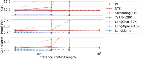
Existing context length extension method separate into two classes. The first type is fine-tuning free methods, including Positional Interpolation (PI) [10], the NTKAware Scale ROPE (NTK) [59], and StreamingLLM [65]. The second type is fine-tuning methods, including LongChat [35], LongAlpaca [11], YaRN [50], and LongLlama [11]. Additional methods such as activation beacon do tune a network seperate from the LLM [68]. As shown in Figure 3, fine-tuning methods achieve better performances than that of fine-tuning free methods at lengths that they have been fine-tuned on. However, fine-tuning methods suffer from a high computational cost and require a potentially intractable amount of GPU memory during fine-tuning.

Refer to caption
Figure 3: Lines in red are fine-tuning free methods and lines in blue are fine-tuning methods. Fine-tuning methods achieve better performances than fine-tuning free method but often suffer from out of memory issues [10, 59, 65, 35, 11, 50, 68, 58]. Lower values are better across all three tasks.

3 Background

We first give a concise introduction to the state-space models, the residual networks, and the adjoint method.

3.1 State-space models

While our method generally applies to all recurrent models, we illustrate the idea using state-space models (SSM\mathrm{SSM}s), which have shown performances at least on par with transformers at small to medium scale [14]. Given an input token sequence {𝐱t}t=1T\{\mathbf{x}_{t}\}_{t=1}^{T}, the SSM\mathrm{SSM}s first calculate the corresponding matrices 𝐀t\mathbf{A}^{t}, 𝐁t\mathbf{B}^{t}, and 𝐂t\mathbf{C}^{t} to evolve the dynamics as follows:

𝐀t=𝓐(𝐱t);𝐁t=𝓑(𝐱t);𝐂t=𝓒(𝐱t).\displaystyle\mathbf{A}^{t}=\boldsymbol{\mathcal{A}}(\mathbf{x}^{t});\;\mathbf{B}^{t}=\boldsymbol{\mathcal{B}}(\mathbf{x}^{t});\;\mathbf{C}^{t}=\boldsymbol{\mathcal{C}}(\mathbf{x}^{t}).

The SSM\mathrm{SSM}s evolve a latent dynamics 𝐡t\mathbf{h}^{t}, whose initial condition 𝐡0\mathbf{h}^{0} is often assumed to be zero. With 𝐡0\mathbf{h}^{0} and 𝐀t,𝐁t\mathbf{A}^{t},\,\mathbf{B}^{t} defined, the dynamics evolves as:

𝐡t=𝐀t𝐡t1+𝐁t𝐱t.\displaystyle\mathbf{h}^{t}=\mathbf{A}^{t}\mathbf{h}^{t-1}+\mathbf{B}^{t}\mathbf{x}^{t}.

The matrices 𝐂t\mathbf{C}^{t} then maps the latent dynamics 𝐡t\mathbf{h}^{t} back to token space as 𝐲t=𝐂t𝐡t\mathbf{y}^{t}=\mathbf{C}^{t}\mathbf{h}^{t}, with 𝐲t\mathbf{y}^{t} being the predicted token at tt. For a sequence of TT tokens, we denote:

𝐀\displaystyle\mathbf{A} =(𝐀1,𝐀2,,𝐀T),𝐁=(𝐁1,𝐁2,,𝐁T),𝐂=(𝐂1,𝐂2,,𝐂T),\displaystyle=(\mathbf{A}^{1},\mathbf{A}^{2},\dots,\mathbf{A}^{T}),\;\mathbf{B}=(\mathbf{B}^{1},\mathbf{B}^{2},\dots,\mathbf{B}^{T}),\;\mathbf{C}=(\mathbf{C}^{1},\mathbf{C}^{2},\dots,\mathbf{C}^{T}),
𝐇\displaystyle\mathbf{H} =(𝐡1,𝐡2,,𝐡T),𝐗=(𝐱1,𝐱2,,𝐱T),𝐘=(𝐲1,𝐲2,,𝐲T).\displaystyle=(\mathbf{h}^{1},\mathbf{h}^{2},\dots,\mathbf{h}^{T}),\;\mathbf{X}=(\mathbf{x}^{1},\mathbf{x}^{2},\dots,\mathbf{x}^{T}),\;\mathbf{Y}=(\mathbf{y}^{1},\mathbf{y}^{2},\dots,\mathbf{y}^{T}).

In the most general case, we have 𝐇T×N,𝐀T×N×N,𝐁T×N×P,𝐂T×P×N,𝐗T×P,𝐘T×P\mathbf{H}\in\mathbb{R}^{T\times N},\mathbf{A}\in\mathbb{R}^{T\times N\times N},\mathbf{B}\in\mathbb{R}^{T\times N\times P},\mathbf{C}\in\mathbb{R}^{T\times P\times N},\mathbf{X}\in\mathbb{R}^{T\times P},\mathbf{Y}\in\mathbb{R}^{T\times P}, where NN is the hidden state dimension, and PP is the input/output dimension. We evolve the dynamics for t=1,,Tt=1,\dots,T, and assume that 𝐡0\mathbf{h}^{0} is a fixed and predefined constant.

The input to an SSM\mathrm{SSM} is 𝐗\mathbf{X} and 𝐡0\mathbf{h}^{0}, and the output is 𝐘\mathbf{Y}. We define SSM()\mathrm{SSM}(\cdot) as performing the following five steps:

  1. 1.

    {𝐀t}t=1T={𝓐(𝐱t)}t=1T,\begin{aligned} \{\mathbf{A}^{t}\}_{t=1}^{T}=\{\boldsymbol{\mathcal{A}}(\mathbf{x}^{t})\}_{t=1}^{T},\end{aligned}

  2. 2.

    {𝐁t}t=1T={𝓑(𝐱t)}t=1T,\begin{aligned} \{\mathbf{B}^{t}\}_{t=1}^{T}=\{\boldsymbol{\mathcal{B}}(\mathbf{x}^{t})\}_{t=1}^{T},\end{aligned}

  3. 3.

    {𝐂t}t=1T={𝓒(𝐱t)}t=1T,\begin{aligned} \{\mathbf{C}^{t}\}_{t=1}^{T}=\{\boldsymbol{\mathcal{C}}(\mathbf{x}^{t})\}_{t=1}^{T},\end{aligned}

  4. 4.

    {𝐡t}t=1T={𝐀t𝐡t1+𝐁t𝐱t}t=1T;\begin{aligned} \{\mathbf{h}^{t}\}_{t=1}^{T}=\{\mathbf{A}^{t}\mathbf{h}^{t-1}+\mathbf{B}^{t}\mathbf{x}^{t}\}_{t=1}^{T};\end{aligned}

  5. 5.

    {𝐲t}t=1T={𝐂t𝐡t}t=1T.\begin{aligned} \{\mathbf{y}^{t}\}_{t=1}^{T}=\{\mathbf{C}^{t}\mathbf{h}^{t}\}_{t=1}^{T}.\end{aligned}

The input to the five steps is 𝐗\mathbf{X}, and the output is 𝐘\mathbf{Y}. We can then write SSM(𝐗)=𝐘\mathrm{SSM}(\mathbf{X})=\mathbf{Y}. SSMs decrease the quadratic computational complexity with sequence length on transformers to linear and decrease the large inference-time memory requirements from the key-value cache. SSM-based models at a small to medium scale have shown performances on par with or better than transformer-based models. For instance, [51, 1] shows that SSM-based mixture-of-experts (MOE) model outperforms baseline transformer-based MOE model on model sizes as big as 2400M parameters. [62] performed an extensive empirical study and found that while SSMs outperform transformers on various tasks, they underperform on tasks which require strong copying, in-context learning, or long-context reasoning abilities. [62] also experimented with a SSM-transformer hybrid model, which outperforms transformers and is up to eight times faster when generating tokens at inference time. [37] trained a 52B parameter model and further affirmed the hybrid models performances.

3.2 Residual Networks

In practice, we have KK SSM\mathrm{SSM}s stacked together, and we have a large language head (LLH) Ω𝕋×P\Omega\in\mathbb{R}^{\mathbb{T}\times P}, where 𝕋\mathbb{T} is the number of all possible tokens. To predict a token, we have 𝐨t=Ω𝐲^Kt\mathbf{o}^{t}=\Omega\hat{\mathbf{y}}_{K}^{t}. Define (𝐲K1,,𝐲KT)=𝐘K(\mathbf{y}_{K}^{1},\dots,\mathbf{y}_{K}^{T})=\mathbf{Y}_{K}, a ResNet computes 𝐘K\mathbf{Y}_{K} as follows:

(𝐲K1,,𝐲KT)\displaystyle(\mathbf{y}_{K}^{1},\dots,\mathbf{y}_{K}^{T}) =𝐘K1+SSMK(𝐘^K1)\displaystyle=\mathbf{Y}_{K-1}+\mathrm{SSM}_{K}(\hat{\mathbf{Y}}_{K-1})
=𝐘0+SSM1(𝐘^0)++SSMK(𝐘^K1)\displaystyle=\mathbf{Y}_{0}+\mathrm{SSM}_{1}(\hat{\mathbf{Y}}_{0})+\dots+\mathrm{SSM}_{K}(\hat{\mathbf{Y}}_{K-1})
=𝐘0+k=1KSSMk(𝐘^k1)=𝐘0+k=1K𝐘~k,\displaystyle=\mathbf{Y}_{0}+\sum_{k=1}^{K}\mathrm{SSM}_{k}(\hat{\mathbf{Y}}_{k-1})=\mathbf{Y}_{0}+\sum_{k=1}^{K}\tilde{\mathbf{Y}}_{k},

where 𝐘^k=(𝐲^k1,,𝐲^kT)=(Norm(𝐲k1),,Norm(𝐲kT))\hat{\mathbf{Y}}_{k}=(\hat{\mathbf{y}}_{k}^{1},\dots,\hat{\mathbf{y}}_{k}^{T})=(\mathrm{Norm}(\mathbf{y}_{k}^{1}),\dots,\mathrm{Norm}(\mathbf{y}_{k}^{T})) and SSMk(𝐘^k1)=𝐘~k\mathrm{SSM}_{k}(\hat{\mathbf{Y}}_{k-1})=\tilde{\mathbf{Y}}_{k}. Therefore, for a latent state at time tt we have 𝐲Kt=𝐲0t+k=1K𝐲~kt\mathbf{y}_{K}^{t}=\mathbf{y}_{0}^{t}+\sum_{k=1}^{K}\tilde{\mathbf{y}}_{k}^{t}.

ResNet has been the foundation of numerous modern networks, including the transformers, diffusion models, segmentation models, SSMs, and more [29, 26, 34, 48]. ResNet’s residual structure allows for a separation between gradients of each layer by applying differentiation on summations.

3.3 Adjoint method

The adjoint method is concerned with optimizing 𝐲(𝐡(𝜽),𝜽)\mathbf{y}(\mathbf{h}(\boldsymbol{\theta}),\boldsymbol{\theta}) with respect to 𝜽\boldsymbol{\theta}, where 𝐡(𝜽)P\mathbf{h}(\boldsymbol{\theta})\in\mathbb{R}^{P} is the solution to 𝐟(𝐡(𝜽),𝜽)=0\mathbf{f}(\mathbf{h}(\boldsymbol{\theta}),\boldsymbol{\theta})=0 [8]. To employ gradient based algorithms like the stochastic gradient descent (SGD) or the Adam, we compute the derivative of 𝐲\mathbf{y} regarding 𝜽|𝜽|\boldsymbol{\theta}\in\mathbb{R}^{|\boldsymbol{\theta}|}:

d𝐲d𝜽=𝐲𝜽+𝐲𝐡𝐡𝜽,\frac{\mathrm{d}\mathbf{y}}{\mathrm{d}\boldsymbol{\theta}}=\frac{\partial\mathbf{y}}{\partial\boldsymbol{\theta}}+\frac{\partial\mathbf{y}}{\partial\mathbf{h}}\frac{\partial\mathbf{h}}{\partial\boldsymbol{\theta}}, (1)

with d\mathrm{d} being the total derivative, and \partial being the partial derivative. The adjoint method converts computing d𝐲/d𝜽\mathrm{d}\mathbf{y}/\mathrm{d}\boldsymbol{\theta} to solving an adjoint equation. In our case, we need the adjoint method for recurrence relations, where 𝐲\mathbf{y} is given by 𝐲=𝐲t𝐲(𝐡t(𝜽),𝜽)\mathbf{y}=\mathbf{y}^{t}\equiv\mathbf{y}(\mathbf{h}^{t}(\boldsymbol{\theta}),\boldsymbol{\theta}), and 𝐡\mathbf{h} is given by

{𝐡0=𝐛(𝜽),𝐡t=𝐟(t,𝐡t1,𝜽).\begin{cases}\mathbf{h}^{0}&=\mathbf{b}(\boldsymbol{\theta}),\\ \mathbf{h}^{t}&=\mathbf{f}(t,\mathbf{h}^{t-1},\boldsymbol{\theta}).\end{cases} (2)

We have

d𝐟(t,𝐡t1,𝜽)d𝜽=𝐟(t,𝐡t1,𝜽)𝜽+𝐟(t,𝐡t1,𝜽)𝐡t1𝐡t1𝜽.\frac{\mathrm{d}\mathbf{f}(t,\mathbf{h}^{t-1},\boldsymbol{\theta})}{\mathrm{d}\boldsymbol{\theta}}=\frac{\partial\mathbf{f}(t,\mathbf{h}^{t-1},\boldsymbol{\theta})}{\partial\boldsymbol{\theta}}+\frac{\partial\mathbf{f}(t,\mathbf{h}^{t-1},\boldsymbol{\theta})}{\partial\mathbf{h}^{t-1}}\frac{\partial\mathbf{h}^{t-1}}{\partial\boldsymbol{\theta}}. (3)
Proposition 1

[8] When the states 𝐡\mathbf{h} are defined as Equation 2, the gradient of 𝐲\mathbf{y} with respect to 𝛉\boldsymbol{\theta} is given as:

{d𝐲t/d𝜽=𝐲t/𝜽+𝝀0𝐛(𝜽)+i=1t𝝀i(𝐟(i,𝐡i1,𝜽)/𝜽),𝝀t=𝐲t/𝐡t,𝝀i1=𝝀i(𝐟(i,𝐡i1,𝜽)/𝐡i1).\begin{cases}\mathrm{d}\mathbf{y}^{t}/\mathrm{d}\boldsymbol{\theta}&=\partial\mathbf{y}^{t}/\partial\boldsymbol{\theta}+\boldsymbol{\lambda}^{0}\mathbf{b}(\boldsymbol{\theta})+\sum_{i=1}^{t}\boldsymbol{\lambda}^{i}\left(\partial\mathbf{f}(i,\mathbf{h}^{i-1},\boldsymbol{\theta})/\partial\boldsymbol{\theta}\right),\\ \boldsymbol{\lambda}^{t}&=\partial\mathbf{y}^{t}/\partial\mathbf{h}^{t},\\ \boldsymbol{\lambda}^{i-1}&=\boldsymbol{\lambda}^{i}\left(\partial\mathbf{f}(i,\mathbf{h}^{i-1},\boldsymbol{\theta})/\partial\mathbf{h}^{i-1}\right).\end{cases} (4)

Equivalently, we have 𝛌i=(𝐲t/𝐡t)(j=ti+1(𝐟(j,𝐡j1,𝛉)/𝐡j1))\boldsymbol{\lambda}^{i}=(\partial\mathbf{y}^{t}/\partial\mathbf{h}^{t})\left(\prod_{j=t}^{i+1}\left(\partial\mathbf{f}(j,\mathbf{h}^{j-1},\boldsymbol{\theta})/\partial\mathbf{h}^{j-1}\right)\right) [32].

After computing adjoint states {𝝀i}i=0t\{\boldsymbol{\lambda}^{i}\}_{i=0}^{t}, the computation of the elements of 𝝀i(𝐟(i,𝐡i1,𝜽)/𝜽)\boldsymbol{\lambda}^{i}(\partial\mathbf{f}(i,\mathbf{h}^{i-1},\boldsymbol{\theta})/\partial\boldsymbol{\theta}) are independent, allowing parallelism. This computation is a vector-Jacobian product (vjp\mathrm{vjp}), with 𝝀i\boldsymbol{\lambda}^{i} as the vector and 𝐟(i,𝐡i1,𝜽)/𝜽\partial\mathbf{f}(i,\mathbf{h}^{i-1},\boldsymbol{\theta})/\partial\boldsymbol{\theta} as the Jacobian. vjp\mathrm{vjp}s can be evaluated with the reverse-mode automatic differentiation and initializing the reverse phase with 𝝀i\boldsymbol{\lambda}^{i} [3]. As each vjp\mathrm{vjp} only requires saving their corresponding computation graph, and can be disposed after the computation, we can compute vjp\mathrm{vjp}s in parallel on modern GPUs. We will discuss this in more details in subsection 4.5. Adjoint sharding aims to use the adjoint method to replace backpropagation, which solves:

d𝐲td𝜽\displaystyle\frac{\mathrm{d}\mathbf{y}^{t}}{\mathrm{d}\boldsymbol{\theta}} =𝐲t𝜽+𝐲t𝐡t(𝐟(t,𝐡t1,𝜽)𝜽+𝐟(t,𝐡t1,𝜽)𝒉t1\displaystyle=\frac{\partial\mathbf{y}^{t}}{\partial\boldsymbol{\theta}}+\frac{\partial\mathbf{y}^{t}}{\partial\mathbf{h}^{t}}\biggl{(}\frac{\partial\mathbf{f}(t,\mathbf{h}^{t-1},\boldsymbol{\theta})}{\partial\boldsymbol{\theta}}+\frac{\partial\mathbf{f}(t,\mathbf{h}^{t-1},\boldsymbol{\theta})}{\partial\boldsymbol{h}^{t-1}}
[𝐟(t1,𝐡t2,𝜽)𝜽+𝐟(t1,𝐡t2,𝜽)𝒉t2{𝐟(t2,𝐡t3,𝜽)𝜽+}]).\displaystyle\biggl{[}\frac{\partial\mathbf{f}(t-1,\mathbf{h}^{t-2},\boldsymbol{\theta})}{\partial\boldsymbol{\theta}}+\frac{\partial\mathbf{f}(t-1,\mathbf{h}^{t-2},\boldsymbol{\theta})}{\partial\boldsymbol{h}^{t-2}}\biggl{\{}\frac{\partial\mathbf{f}(t-2,\mathbf{h}^{t-3},\boldsymbol{\theta})}{\partial\boldsymbol{\theta}}+\dots\biggl{\}}\biggl{]}\biggl{)}.

The backpropagation requires a sequential accumulation of the gradients, computing from the outmost layer inwards, therefore needs to save the computation graph for computations at all time tt’s and creates memory bottlenecks.

4 Adjoint sharding

We now introduce the adjoint sharding technique. We first illustrate the method assuming only one layer of SSM\mathrm{SSM}, and generalize to KK layers.

4.1 Adjoint sharding for one SSM

Large scale neural networks are usually trained with the autograd framework [4, 47]. However, this framework suffers from a high memory cost when used with networks of recurrent nature [4]. Although activation checkpointing has been developed, which discards part of the intermediate values and recomputes them later on the fly, the memory cost is still high [30]. We employ the adjoint method for recurrence relations to further reduce the memory cost, and more importantly, to break the temporal dependencies of activations and parallelize their computations.

Define θ=θ𝓐,θ𝓑,θ𝓒\theta=\langle\theta_{\boldsymbol{\mathcal{A}}},\theta_{\boldsymbol{\mathcal{B}}},\theta_{\boldsymbol{\mathcal{C}}}\rangle as 𝓐\boldsymbol{\mathcal{A}}’s, 𝓑\boldsymbol{\mathcal{B}}’s, and 𝓒\boldsymbol{\mathcal{C}}’s parameters, for loss lt=l(𝐲t)l^{t}=l(\mathbf{y}^{t}), in the context of a single-layer SSM\mathrm{SSM}, we prove:

Proposition 2

The gradient dlt/d𝛉\mathrm{d}l^{t}/\mathrm{d}\boldsymbol{\theta} is given as

dltd𝜽=[i=1tvjp𝓐i(dltd𝐲t𝝀t,i𝐡i1)][i=1tvjp𝓑i(dltd𝐲t𝝀t,i𝐱^i)]vjp𝓒t(dltd𝐲t𝐡t),\frac{\mathrm{d}l^{t}}{\mathrm{d}\boldsymbol{\theta}}=\left[\sum_{i=1}^{t}\mathrm{vjp}_{\boldsymbol{\mathcal{A}}^{i}}(\frac{\mathrm{d}l^{t}}{\mathrm{d}\mathbf{y}^{t}}\boldsymbol{\lambda}^{t,i}\otimes\mathbf{h}^{i-1})\right]\oplus\left[\sum_{i=1}^{t}\mathrm{vjp}_{\boldsymbol{\mathcal{B}}^{i}}(\frac{\mathrm{d}l^{t}}{\mathrm{d}\mathbf{y}^{t}}\boldsymbol{\lambda}^{t,i}\otimes\hat{\mathbf{x}}^{i})\right]\oplus\mathrm{vjp}_{\boldsymbol{\mathcal{C}}^{t}}(\frac{\mathrm{d}l^{t}}{\mathrm{d}\mathbf{y}^{t}}\otimes\mathbf{h}^{t}), (5)

where the adjoint state 𝛌t,τ=𝐂t(i=1tτ𝐀t+1i)\boldsymbol{\lambda}^{t,\tau}=\mathbf{C}^{t}(\prod_{i=1}^{t-\tau}\mathbf{A}^{t+1-i}), vjpNeti(v)=vNet𝛉(Inputi)\mathrm{vjp}_{\mathrm{Net}^{i}}(v)=v\cdot\mathrm{Net}_{\boldsymbol{\theta}}(\mathrm{Input}^{i}), with 𝛉\boldsymbol{\theta} being Net\mathrm{Net}’s parameters and ii being the index of Input\mathrm{Input}, \otimes is the vector outer product, and \oplus is vector concatenation.

The proof of proposition 2 is in section A.1. The gradient for parameters of 𝓐\boldsymbol{\mathcal{A}}, and 𝓑\boldsymbol{\mathcal{B}} are each separated into {vjp𝓐i(dltd𝐲t𝝀t,i𝐡i1)}i=1t\{\mathrm{vjp}_{\boldsymbol{\mathcal{A}}^{i}}(\frac{\mathrm{d}l^{t}}{\mathrm{d}\mathbf{y}^{t}}\boldsymbol{\lambda}^{t,i}\otimes\mathbf{h}^{i-1})\}_{i=1}^{t}, {vjp𝓑i(dltd𝐲t𝝀t,i𝐱^i}i=1t\{\mathrm{vjp}_{\boldsymbol{\mathcal{B}}^{i}}(\frac{\mathrm{d}l^{t}}{\mathrm{d}\mathbf{y}^{t}}\boldsymbol{\lambda}^{t,i}\otimes\hat{\mathbf{x}}^{i}\}_{i=1}^{t}, and the gradient for parameters of 𝓒\boldsymbol{\mathcal{C}} only depend on inputs at time tt. After computing the adjoint states, these vjp\mathrm{vjp} computations are separate from each other on both the network and the temporal level.

Refer to caption
Figure 4: The adjoint states are computed sequentially backwards.

4.2 Adjoint sharding for multiple SSMs

We now generalize the results from subsection 4.1 to the general case of KK SSM\mathrm{SSM}s concatenated together. As introduced in subsection 3.2, the outputs of each SSM\mathrm{SSM} layer are added to the results of the last layer and normalized before it is fed into the next layer. Define the loss over all token predictions L=t=1TltL=\sum_{t=1}^{T}l^{t}, using the residual structure we have

dLd𝜽=t=1Tdltd𝐲Ktd𝐲Ktd𝜽=t=1Tdltd𝐲Ktd(𝐲0t+k=1K𝐲~kt)d𝜽=t=1Tdltd𝐲Ktk=1Kd𝐲~ktd𝜽.\displaystyle\frac{\mathrm{d}L}{\mathrm{d}\boldsymbol{\theta}}=\sum_{t=1}^{T}\frac{\mathrm{d}l^{t}}{\mathrm{d}\mathbf{y}_{K}^{t}}\frac{\mathrm{d}\mathbf{y}_{K}^{t}}{\mathrm{d}\boldsymbol{\theta}}=\sum_{t=1}^{T}\frac{\mathrm{d}l^{t}}{\mathrm{d}\mathbf{y}_{K}^{t}}\frac{\mathrm{d}(\mathbf{y}_{0}^{t}+\sum_{k=1}^{K}\tilde{\mathbf{y}}_{k}^{t})}{\mathrm{d}\boldsymbol{\theta}}=\sum_{t=1}^{T}\frac{\mathrm{d}l^{t}}{\mathrm{d}\mathbf{y}_{K}^{t}}\sum_{k=1}^{K}\frac{\mathrm{d}\tilde{\mathbf{y}}_{k}^{t}}{\mathrm{d}\boldsymbol{\theta}}.

Combining with proposition 2, we have

Proposition 3

The gradient of the total loss LL with respect to the SSM\mathrm{SSM} parameters 𝛉\boldsymbol{\theta} is given as

dLd𝜽=(t=1Tk=1Ki=1tvjp𝓐ki(dltd𝐲Kt𝝀kt,i𝐡ki1))(t=1Tk=1Ki=1tvjp𝓑ki(dltd𝐲Kt𝝀kt,i𝐲^k1i))(t=1Tk=1Kvjp𝓒kt(dltd𝐲Kt𝐡kt)),\begin{split}\frac{\mathrm{d}L}{\mathrm{d}\boldsymbol{\theta}}&=\left(\sum_{t=1}^{T}\sum_{k=1}^{K}\sum_{i=1}^{t}\mathrm{vjp}_{\boldsymbol{\mathcal{A}}^{i}_{k}}(\frac{\mathrm{d}l^{t}}{\mathrm{d}\mathbf{y}_{K}^{t}}\boldsymbol{\lambda}^{t,i}_{k}\otimes\mathbf{h}^{i-1}_{k})\right)\\ &\oplus\left(\sum_{t=1}^{T}\sum_{k=1}^{K}\sum_{i=1}^{t}\mathrm{vjp}_{\boldsymbol{\mathcal{B}}^{i}_{k}}(\frac{\mathrm{d}l^{t}}{\mathrm{d}\mathbf{y}_{K}^{t}}\boldsymbol{\lambda}^{t,i}_{k}\otimes\hat{\mathbf{y}}^{i}_{k-1})\right)\\ &\oplus\left(\sum_{t=1}^{T}\sum_{k=1}^{K}\mathrm{vjp}_{\boldsymbol{\mathcal{C}}^{t}_{k}}(\frac{\mathrm{d}l^{t}}{\mathrm{d}\mathbf{y}_{K}^{t}}\otimes\mathbf{h}^{t}_{k})\right),\end{split} (6)

where the input to vjp𝓒kt(dltd𝐲Kt𝐡kt),vjp𝓐ki(dltd𝐲Kt𝛌kt,i𝐡ki1),andvjp𝓑ki(dltd𝐲Kt𝛌kt,i𝐲^k1i)\mathrm{vjp}_{\boldsymbol{\mathcal{C}}^{t}_{k}}(\frac{\mathrm{d}l^{t}}{\mathrm{d}\mathbf{y}_{K}^{t}}\otimes\mathbf{h}^{t}_{k}),\,\mathrm{vjp}_{\boldsymbol{\mathcal{A}}^{i}_{k}}(\frac{\mathrm{d}l^{t}}{\mathrm{d}\mathbf{y}_{K}^{t}}\boldsymbol{\lambda}^{t,i}_{k}\otimes\mathbf{h}^{i-1}_{k}),\,\mathrm{and}\,\mathrm{vjp}_{\boldsymbol{\mathcal{B}}^{i}_{k}}(\frac{\mathrm{d}l^{t}}{\mathrm{d}\mathbf{y}_{K}^{t}}\boldsymbol{\lambda}^{t,i}_{k}\otimes\hat{\mathbf{y}}^{i}_{k-1}) are computed with the k-th SSM\mathrm{SSM} and the 𝐲^k1i=Norm(𝐲k2i+SSMk1(𝐘^k2)i)\hat{\mathbf{y}}_{k-1}^{i}=\mathrm{Norm}(\mathbf{y}_{k-2}^{i}+\mathrm{SSM}_{k-1}(\hat{\mathbf{Y}}_{k-2})^{i}) (the normalized output sequence of the (k-1)-th SSM\mathrm{SSM}). The adjoint state at layer kk is defined as 𝛌kt,τ=𝐂kt(i=1tτ𝐀kt+1i)\boldsymbol{\lambda}^{t,\tau}_{k}=\mathbf{C}^{t}_{k}(\prod_{i=1}^{t-\tau}\mathbf{A}_{k}^{t+1-i}).

Refer to caption
Figure 5: Computation schematic of dlt/d𝜽𝓐k\mathrm{d}l^{t}/\mathrm{d}\boldsymbol{\theta}_{\boldsymbol{\mathcal{A}}_{k}}, dlt/d𝜽𝓑k\mathrm{d}l^{t}/\mathrm{d}\boldsymbol{\theta}_{\boldsymbol{\mathcal{B}}_{k}}, and dlt/d𝜽𝓒k\mathrm{d}l^{t}/\mathrm{d}\boldsymbol{\theta}_{\boldsymbol{\mathcal{C}}_{k}}.

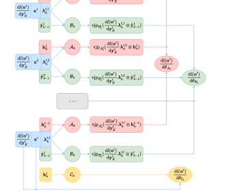
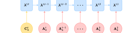
We provide the proof to proposition 3 in section A.2. Define 𝚲kt={𝝀kt,τ}τ=1t\boldsymbol{\Lambda}_{k}^{t}=\{\boldsymbol{\lambda}^{t,\tau}_{k}\}_{\tau=1}^{t}, proposition 3 shows that the gradients of each network’s parameters computed with each token only correlate through the adjoint states {𝚲kt}k,t=1,1K,T\{\boldsymbol{\Lambda}_{k}^{t}\}_{k,t=1,1}^{K,T}. The adjoint states can be easily computed after a forward pass. The adjoint states can also be computed on the fly in the gradient computation phase, as it only depends on 𝐂kt\mathbf{C}_{k}^{t} and 𝐀kt\mathbf{A}_{k}^{t} and has no dependencies on the network Jacobians regarding the network parameters. The adjoint sharding method breaks down the backpropagation computation both layer-wise and token-wise into foundational vjp\mathrm{vjp} computations that do not have any dependencies on each other.

We show a schematic of the computations to dlt/d𝜽𝓐k\mathrm{d}l^{t}/\mathrm{d}\boldsymbol{\theta}_{\boldsymbol{\mathcal{A}}_{k}}, dlt/d𝜽𝓑k\mathrm{d}l^{t}/\mathrm{d}\boldsymbol{\theta}_{\boldsymbol{\mathcal{B}}_{k}}, and dlt/d𝜽𝓒k\mathrm{d}l^{t}/\mathrm{d}\boldsymbol{\theta}_{\boldsymbol{\mathcal{C}}_{k}} in Figure 5 and a schematic for computing the adjoint states in Figure 4.

4.3 Truncated adjoint sharding

One limitation of adjoint sharding is that the number of vjp\mathrm{vjp}s performed increases polynomially regarding the number of tokens TT. In particular, adjoint sharding computes the vjp\mathrm{vjp} for 𝓐𝒌\boldsymbol{\mathcal{A}_{k}} and 𝓑𝒌\boldsymbol{\mathcal{B}_{k}} (1+T)T/2(1+T)T/2 times, and for 𝓒𝒌\boldsymbol{\mathcal{C}_{k}} TT times. When training large networks with many layers and long context length TT, applying adjoint sharding becomes computationally expensive. We propose truncated adjoint sharding, with which we argue that we can get similar results by computing a linearly growing number of vjp\mathrm{vjp}s, and empirically showcase its performance.

Attention mechanisms have suffered from the 𝒪(T2)\mathcal{O}(T^{2}) complexities arising from the self-attention structure [60]. To enable training with longer context lengths, global-local attention has been proposed, where we divide the contexts into sections, and compute the attention between sections rather than tokens [67]. [57] proposed truncated backpropagation through time (T-BPTT) to avoid gradient explosion/vanishing when training with long contexts by only counting a fixed number of state transitions. Here, inspired by global-local attention and T-BPTT, instead of computing the full gradient given in Equation 11, we propose to train the SSM\mathrm{SSM}s to depend on up to T¯\bar{T} states:

dLd𝜽=(t=1Tk=1Kvjp𝓒kt(dltd𝐲Kt𝐡kt))(t=1T¯k=1Ki=1tvjp𝓐ki(dltd𝐲Kt𝝀kt,i𝐡ki1)+t=T¯+1Tk=1Ki=t+1T¯tvjp𝓐ki(dltd𝐲Kt𝝀kt,i𝐡ki1))(t=1T¯k=1Ki=1tvjp𝓑ki(dltd𝐲Kt𝝀kt,i𝐲^k1i)+t=T¯+1Tk=1Ki=t+1T¯tvjp𝓑ki(dltd𝐲Kt𝝀kt,i𝐲^k1i)\begin{split}\frac{\mathrm{d}L}{\mathrm{d}\boldsymbol{\theta}}&=\left(\sum_{t=1}^{T}\sum_{k=1}^{K}\mathrm{vjp}_{\boldsymbol{\mathcal{C}}^{t}_{k}}(\frac{\mathrm{d}l^{t}}{\mathrm{d}\mathbf{y}_{K}^{t}}\otimes\mathbf{h}^{t}_{k})\right)\\ &\oplus\left(\sum_{t=1}^{\bar{T}}\sum_{k=1}^{K}\sum_{i=1}^{t}\mathrm{vjp}_{\boldsymbol{\mathcal{A}}^{i}_{k}}(\frac{\mathrm{d}l^{t}}{\mathrm{d}\mathbf{y}_{K}^{t}}\boldsymbol{\lambda}^{t,i}_{k}\otimes\mathbf{h}^{i-1}_{k})+\sum_{t=\bar{T}+1}^{T}\sum_{k=1}^{K}\sum_{i=t+1-\bar{T}}^{t}\mathrm{vjp}_{\boldsymbol{\mathcal{A}}^{i}_{k}}(\frac{\mathrm{d}l^{t}}{\mathrm{d}\mathbf{y}_{K}^{t}}\boldsymbol{\lambda}^{t,i}_{k}\otimes\mathbf{h}^{i-1}_{k})\right)\\ &\oplus\left(\sum_{t=1}^{\bar{T}}\sum_{k=1}^{K}\sum_{i=1}^{t}\mathrm{vjp}_{\boldsymbol{\mathcal{B}}^{i}_{k}}(\frac{\mathrm{d}l^{t}}{\mathrm{d}\mathbf{y}_{K}^{t}}\boldsymbol{\lambda}^{t,i}_{k}\otimes\hat{\mathbf{y}}^{i}_{k-1})+\sum_{t=\bar{T}+1}^{T}\sum_{k=1}^{K}\sum_{i=t+1-\bar{T}}^{t}\mathrm{vjp}_{\boldsymbol{\mathcal{B}}^{i}_{k}}(\frac{\mathrm{d}l^{t}}{\mathrm{d}\mathbf{y}_{K}^{t}}\boldsymbol{\lambda}^{t,i}_{k}\otimes\hat{\mathbf{y}}^{i}_{k-1}\right)\end{split} (7)

As shown in Equation 7 above, we perform the same computations for t=1,,T¯t=1,\dots,\bar{T} as before, and only perform the vjp\mathrm{vjp}s back to the last T¯\bar{T} states for t>T¯t>\bar{T}. With truncated adjoint sharding, we perform T¯T+T¯(T¯1)/2\bar{T}T+\bar{T}(\bar{T}-1)/2 vjp\mathrm{vjp}s, which grows linearly. We show the number of vjp\mathrm{vjp}s performed with and without truncated adjoint sharding in Figure 6. When T¯=2000\bar{T}=2000, truncated adjoint sharding reduces 64%64\% of the vjp\mathrm{vjp}s when training with a context length of 10K10\mathrm{K}.

The essence of the truncated adjoint sharding method is that we only explicitly count gradients related to the last T¯\bar{T} states. As each state depends on its prior state, states still implicitly depend on all their prior states. We leave investigation of T¯\bar{T}’s impact on performances for future works.

4.4 Distributed training

We now discuss how to distribute the storage and compute of the adjoint sharding method, assuming that we have Υ\Upsilon GPUs. Given the networks {𝒜k,k,𝒞k}k=1K\{\mathcal{A}_{k},\mathcal{B}_{k},\mathcal{C}_{k}\}_{k=1}^{K}, initial tokens {𝐲^0t}t=1T={Norm(𝐱t)}t=1T\{\hat{\mathbf{y}}_{0}^{t}\}_{t=1}^{T}=\{\mathrm{Norm}(\mathbf{x}^{t})\}_{t=1}^{T}, and initial conditions {𝐡k0}k=1K\{\mathbf{h}^{0}_{k}\}_{k=1}^{K} (usually set to 𝟎\mathbf{0}), we can call algorithm 1 to get all necessary vectors for computing the gradient with adjoint sharding.

Algorithm 1 Forward step in evaluation mode on a distributed system
1:Inputs: {𝐲^0t}t=1T\{\hat{\mathbf{y}}_{0}^{t}\}_{t=1}^{T}, {𝐡k0}k=1K\{\mathbf{h}^{0}_{k}\}_{k=1}^{K}, {𝒜k,k,𝒞k}k=1K\{\mathcal{A}_{k},\mathcal{B}_{k},\mathcal{C}_{k}\}_{k=1}^{K}, Ω\Omega
2:On devices υ=1,,Υ\upsilon=1,\dots,\Upsilon, in parallel do
3:for SSM model index k=(υ1)(K//Υ)+1,,υ(K//Υ)k=(\upsilon-1)(K//\Upsilon)+1,\dots,\upsilon(K//\Upsilon) do
4:     for Time step index t=1,,Tt=1,\dots,T do
5:         Compute: 𝐀kt=𝒜k(𝐲^k1t)\mathbf{A}_{k}^{t}=\mathcal{A}_{k}(\hat{\mathbf{y}}_{k-1}^{t}); 𝐁kt=k(𝐲^k1t)\mathbf{B}_{k}^{t}=\mathcal{B}_{k}(\hat{\mathbf{y}}_{k-1}^{t}); 𝐂kt=𝒞k(𝐲^k1t)\mathbf{C}_{k}^{t}=\mathcal{C}_{k}(\hat{\mathbf{y}}_{k-1}^{t}); 𝐡kt=𝐀kt𝐡kt1+𝐁kt𝐲^k1t\mathbf{h}_{k}^{t}=\mathbf{A}_{k}^{t}\mathbf{h}_{k}^{t-1}+\mathbf{B}_{k}^{t}\hat{\mathbf{y}}_{k-1}^{t}; 𝐲kt=𝐂kt𝐡kt\mathbf{y}_{k}^{t}=\mathbf{C}_{k}^{t}\mathbf{h}_{k}^{t}.
6:         Compute: 𝐲kt=𝐲k1t+𝐲~kt\mathbf{y}_{k}^{t}=\mathbf{y}_{k-1}^{t}+\tilde{\mathbf{y}}_{k}^{t}.
7:         Compute: 𝐲^kt=Norm(𝐲kt)\hat{\mathbf{y}}_{k}^{t}=\mathrm{Norm}(\mathbf{y}_{k}^{t}).
8:     end for
9:end for
10:Store: {𝐡kt}(t,k)=(1,(υ1)(K//Υ)+1)T,υ(K//Υ)\{\mathbf{h}_{k}^{t}\}_{(t,k)=(1,(\upsilon-1)(K//\Upsilon)+1)}^{T,\upsilon(K//\Upsilon)}, {𝐂kt}(t,k)=(1,(υ1)(K//Υ)+1)T,υ(K//Υ)\{\mathbf{C}_{k}^{t}\}_{(t,k)=(1,(\upsilon-1)(K//\Upsilon)+1)}^{T,\upsilon(K//\Upsilon)}, {𝐲^kt}(t,k)=(1,(υ1)(K//Υ))T,υ(K//Υ)1\{\hat{\mathbf{y}}_{k}^{t}\}_{(t,k)=(1,(\upsilon-1)(K//\Upsilon))}^{T,\upsilon(K//\Upsilon)-1}, {𝐀kt}(t,k)=(2,(υ1)(K//Υ)+1)T,υ(K//Υ)\{\mathbf{A}_{k}^{t}\}_{(t,k)=(2,(\upsilon-1)(K//\Upsilon)+1)}^{T,\upsilon(K//\Upsilon)} on device υ\upsilon.
11:Pass: {𝐲υ(K//Υ)1t}t=1T\{\mathbf{y}_{\upsilon(K//\Upsilon)-1}^{t}\}_{t=1}^{T}, {𝐲^υ(K//Υ)1t}t=1T\{\hat{\mathbf{y}}_{\upsilon(K//\Upsilon)-1}^{t}\}_{t=1}^{T} to device υ+1\upsilon+1
12:for Time step index t=1,,Tt=1,\dots,T do
13:     Compute: {𝐨t=Ω𝐲Kt}t=1T\{\mathbf{o}^{t}=\Omega\mathbf{y}_{K}^{t}\}_{t=1}^{T}, {l(𝐨t)}\{l(\mathbf{o}^{t})\}, {dl(𝐨t)d𝐲Kt}t=1T\{\frac{\mathrm{d}l(\mathbf{o}^{t})}{\mathrm{d}\mathbf{y}_{K}^{t}}\}_{t=1}^{T}.
14:end for
15:Store: {dl(𝐨t)d𝐲Kt}t=1T\{\frac{\mathrm{d}l(\mathbf{o}^{t})}{\mathrm{d}\mathbf{y}_{K}^{t}}\}_{t=1}^{T} on all Υ\Upsilon devices.
Algorithm 2 Evaluating adjoint states for token index tt and ResNet index kk with truncated adjoint sharding T¯\bar{T}
1:Inputs: tt, kk, T¯\bar{T}, 𝐂kt\mathbf{C}_{k}^{t}, {𝐀ki}i=t+2T¯t\{\mathbf{A}^{i}_{k}\}_{i=t+2-\bar{T}}^{t}
2:Initialize adjoint state 𝝀kt,t=𝐂kt\boldsymbol{\lambda}_{k}^{t,t}=\mathbf{C}_{k}^{t}
3:Compute: intermediate values:
4:𝜻T¯=(𝐀kt𝐀kt1𝐀kt+2T¯,𝐀kt𝐀kt1𝐀kt+3T¯,,𝐀kt𝐀kt1,𝐀kt,𝕀)\boldsymbol{\zeta}^{\bar{T}}=(\mathbf{A}_{k}^{t}\mathbf{A}_{k}^{t-1}\dots\mathbf{A}_{k}^{t+2-\bar{T}},\mathbf{A}_{k}^{t}\mathbf{A}_{k}^{t-1}\dots\mathbf{A}_{k}^{t+3-\bar{T}},\dots,\mathbf{A}_{k}^{t}\mathbf{A}_{k}^{t-1},\mathbf{A}_{k}^{t},\mathbb{I}).
5:Compute: adjoint states 𝚲¯kT¯=(𝝀kt,t+1T¯,𝝀kt,t+2T¯,,𝝀kt,t)=𝐂kt𝜻T¯\bar{\boldsymbol{\Lambda}}_{k}^{\bar{T}}=(\boldsymbol{\lambda}_{k}^{t,t+1-\bar{T}},\boldsymbol{\lambda}_{k}^{t,t+2-\bar{T}},\dots,\boldsymbol{\lambda}_{k}^{t,t})=\mathbf{C}_{k}^{t}\boldsymbol{\zeta}^{\bar{T}}.
6:Return: 𝚲¯kT¯\bar{\boldsymbol{\Lambda}}_{k}^{\bar{T}}.
Algorithm 3 Evaluating the vjp\mathrm{vjp}’s for token index tt and ResNet index kk with truncated adjoint sharding T¯\bar{T}
1:Inputs: tt, kk, T¯\bar{T}, dl(𝐨t)d𝐲Kt\frac{\mathrm{d}l(\mathbf{o}^{t})}{\mathrm{d}\mathbf{y}_{K}^{t}}, {𝐡ki}i=tT¯t\{\mathbf{h}_{k}^{i}\}_{i=t-\bar{T}}^{t}, 𝐂kt\mathbf{C}_{k}^{t}, {𝐲k1i}i=t+1T¯t\{\mathbf{y}^{i}_{k-1}\}_{i=t+1-\bar{T}}^{t}, {𝐀ki}i=t+2T¯t\{\mathbf{A}^{i}_{k}\}_{i=t+2-\bar{T}}^{t}
2:Call alg. 2 to compute {𝝀kt,i}i=t+1T¯t\{\boldsymbol{\lambda}_{k}^{t,i}\}_{i=t+1-\bar{T}}^{t}
3:Compute: dl(𝐨t)d𝐲Kt𝐡kt\frac{\mathrm{d}l(\mathbf{o}^{t})}{\mathrm{d}\mathbf{y}_{K}^{t}}\otimes\mathbf{h}^{t}_{k}, {dl(𝐨t)d𝐲Kt𝝀kt,i𝐡ki1}i=t+1T¯t\{\frac{\mathrm{d}l(\mathbf{o}^{t})}{\mathrm{d}\mathbf{y}_{K}^{t}}\boldsymbol{\lambda}^{t,i}_{k}\otimes\mathbf{h}^{i-1}_{k}\}_{i=t+1-\bar{T}}^{t}, {dl(𝐨t)d𝐲Kt𝝀kt,i𝐲^k1i}i=t+1T¯t\{\frac{\mathrm{d}l(\mathbf{o}^{t})}{\mathrm{d}\mathbf{y}_{K}^{t}}\boldsymbol{\lambda}^{t,i}_{k}\otimes\hat{\mathbf{y}}^{i}_{k-1}\}_{i=t+1-\bar{T}}^{t}
4:Compute:(vjp𝐂kt(dl(𝐨t)d𝐲Kt𝐡kt),i=t+1T¯tvjp𝐀ki(dl(𝐨t)d𝐲Kt𝝀kt,i𝐡ki1),i=t+1T¯tvjp𝐁ki(dl(𝐨t)d𝐲Kt𝝀kt,i𝐲^k1i))\left(\mathrm{vjp}_{\mathbf{C}^{t}_{k}}(\frac{\mathrm{d}l(\mathbf{o}^{t})}{\mathrm{d}\mathbf{y}_{K}^{t}}\otimes\mathbf{h}^{t}_{k}),\,\sum_{i=t+1-\bar{T}}^{t}\mathrm{vjp}_{\mathbf{A}^{i}_{k}}(\frac{\mathrm{d}l(\mathbf{o}^{t})}{\mathrm{d}\mathbf{y}_{K}^{t}}\boldsymbol{\lambda}^{t,i}_{k}\otimes\mathbf{h}^{i-1}_{k}),\,\sum_{i=t+1-\bar{T}}^{t}\mathrm{vjp}_{\mathbf{B}^{i}_{k}}(\frac{\mathrm{d}l(\mathbf{o}^{t})}{\mathrm{d}\mathbf{y}_{K}^{t}}\boldsymbol{\lambda}^{t,i}_{k}\otimes\hat{\mathbf{y}}^{i}_{k-1})\right)
5:Return: (vjp𝐂kt(dl(𝐨t)d𝐲Kt𝐡kt),i=t+1T¯tvjp𝐀ki(dl(𝐨t)d𝐲Ktλkt,i𝐡ki1),i=t+1T¯tvjp𝐁ki(dl(𝐨t)d𝐲Ktλkt,i𝐲^k1i))\left(\mathrm{vjp}_{\mathbf{C}^{t}_{k}}(\frac{\mathrm{d}l(\mathbf{o}^{t})}{\mathrm{d}\mathbf{y}_{K}^{t}}\otimes\mathbf{h}^{t}_{k}),\,\sum_{i=t+1-\bar{T}}^{t}\mathrm{vjp}_{\mathbf{A}^{i}_{k}}(\frac{\mathrm{d}l(\mathbf{o}^{t})}{\mathrm{d}\mathbf{y}_{K}^{t}}\boldsymbol{\lambda}^{t,i}_{k}\otimes\mathbf{h}^{i-1}_{k}),\,\sum_{i=t+1-\bar{T}}^{t}\mathrm{vjp}_{\mathbf{B}^{i}_{k}}(\frac{\mathrm{d}l(\mathbf{o}^{t})}{\mathrm{d}\mathbf{y}_{K}^{t}}\boldsymbol{\lambda}^{t,i}_{k}\otimes\hat{\mathbf{y}}^{i}_{k-1})\right)
Algorithm 4 Evaluating dLd𝜽\frac{\mathrm{d}L}{\mathrm{d}\boldsymbol{\theta}} with truncated adjoint sharding T¯\bar{T} on Υ\Upsilon devices
1:Inputs: {𝐲0t}t=1T\{\mathbf{y}_{0}^{t}\}_{t=1}^{T}, {𝐡k0}k=1K\{\mathbf{h}^{0}_{k}\}_{k=1}^{K}, {𝒜k,k,𝒞k}k=1K\{\mathcal{A}_{k},\mathcal{B}_{k},\mathcal{C}_{k}\}_{k=1}^{K}, Ω\Omega, T¯\bar{T}, Υ\Upsilon
2:Call alg. 1 for {𝐀kt,𝐂kt,𝐡kt,𝐲^kt}(t,k)=(1,1)(T,K),{dl(𝐨t)d𝐲Kt}t=1T\{\mathbf{A}_{k}^{t},\mathbf{C}_{k}^{t},\mathbf{h}_{k}^{t},\hat{\mathbf{y}}_{k}^{t}\}_{(t,k)=(1,1)}^{(T,K)},\{\frac{\mathrm{d}l(\mathbf{o}^{t})}{\mathrm{d}\mathbf{y}_{K}^{t}}\}_{t=1}^{T} and saved on each GPU device.
3:On each device υ\upsilon, in parallel do
4:Initialize gradient dLd𝜽\frac{\mathrm{d}L}{\mathrm{d}\boldsymbol{\theta}}
5:for Time step index t=1,,T¯t=1,\dots,\bar{T}, layer index k=(υ1)(K//Υ)+1,,υ(K//Υ)k=(\upsilon-1)(K//\Upsilon)+1,\dots,\upsilon(K//\Upsilon) do
6:     Call alg. 3 for Ξ=(vjp𝐂kt(dl(𝐨t)d𝐲Kt𝐡kt),i=1tvjp𝐀ki(dl(𝐨t)d𝐲Kt𝝀kt,i𝐡ki1),i=1tvjp𝐁ki(dl(𝐨t)d𝐲Kt𝝀kt,i𝐲^k1i))\Xi=\left(\mathrm{vjp}_{\mathbf{C}^{t}_{k}}(\frac{\mathrm{d}l(\mathbf{o}^{t})}{\mathrm{d}\mathbf{y}_{K}^{t}}\otimes\mathbf{h}^{t}_{k}),\,\sum_{i=1}^{t}\mathrm{vjp}_{\mathbf{A}^{i}_{k}}(\frac{\mathrm{d}l(\mathbf{o}^{t})}{\mathrm{d}\mathbf{y}_{K}^{t}}\boldsymbol{\lambda}^{t,i}_{k}\otimes\mathbf{h}^{i-1}_{k}),\,\sum_{i=1}^{t}\mathrm{vjp}_{\mathbf{B}^{i}_{k}}(\frac{\mathrm{d}l(\mathbf{o}^{t})}{\mathrm{d}\mathbf{y}_{K}^{t}}\boldsymbol{\lambda}^{t,i}_{k}\otimes\hat{\mathbf{y}}^{i}_{k-1})\right)
7:     Compute: dLd𝜽+=Ξ\frac{\mathrm{d}L}{\mathrm{d}\boldsymbol{\theta}}+=\Xi
8:end for
9:for Time step index t=T¯+1,,Tt=\bar{T}+1,\dots,T, layer index k=(υ1)(K//Υ)+1,,υ(K//Υ)k=(\upsilon-1)(K//\Upsilon)+1,\dots,\upsilon(K//\Upsilon) do
10:      Call alg. 3 for Ξ=(vjp𝐂kt(dl(𝐨t)d𝐲Kt𝐡kt),i=t+1T¯tvjp𝐀ki(dl(𝐨t)d𝐲Kt𝝀kt,i𝐡ki1),\Xi=\Biggl{(}\mathrm{vjp}_{\mathbf{C}^{t}_{k}}(\frac{\mathrm{d}l(\mathbf{o}^{t})}{\mathrm{d}\mathbf{y}_{K}^{t}}\otimes\mathbf{h}^{t}_{k}),\,\sum_{i=t+1-\bar{T}}^{t}\mathrm{vjp}_{\mathbf{A}^{i}_{k}}(\frac{\mathrm{d}l(\mathbf{o}^{t})}{\mathrm{d}\mathbf{y}_{K}^{t}}\boldsymbol{\lambda}^{t,i}_{k}\otimes\mathbf{h}^{i-1}_{k}), i=t+1T¯tvjp𝐁ki(dl(𝐨t)d𝐲Kt𝝀kt,i𝐲^k1i))\sum_{i=t+1-\bar{T}}^{t}\mathrm{vjp}_{\mathbf{B}^{i}_{k}}(\frac{\mathrm{d}l(\mathbf{o}^{t})}{\mathrm{d}\mathbf{y}_{K}^{t}}\boldsymbol{\lambda}^{t,i}_{k}\otimes\hat{\mathbf{y}}^{i}_{k-1})\Biggl{)}
11:     Compute: dLd𝜽+=Ξ\frac{\mathrm{d}L}{\mathrm{d}\boldsymbol{\theta}}+=\Xi
12:end for
13:Return: dLdθ\frac{\mathrm{d}L}{\mathrm{d}\boldsymbol{\theta}}

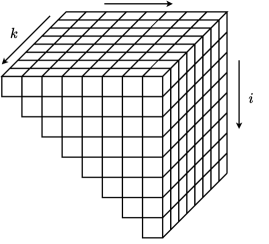
As shown in algorithm 3, to compute the vjp\mathrm{vjp}s’ for token index tt and ResNet index kk, we only need t,k,dl(𝐨t)/d𝐲Kt,{𝐡ki}i=0t,𝐂kt,{𝐲^k1i}i=1t,{𝐀ki}i=2tt,k,\mathrm{d}l(\mathbf{o}^{t})/\mathrm{d}\mathbf{y}_{K}^{t},\{\mathbf{h}_{k}^{i}\}_{i=0}^{t},\mathbf{C}_{k}^{t},\{\hat{\mathbf{y}}_{k-1}^{i}\}_{i=1}^{t},\{\mathbf{A}_{k}^{i}\}_{i=2}^{t}. To compute all the gradients for layer kk, we only need 𝐀\mathbf{A}, 𝐡\mathbf{h}, and 𝐂\mathbf{C} from the kk-th layer, and 𝐲^\hat{\mathbf{y}} from the k1k-1-th layer. Therefore, we can divide the KK layers into Υ\Upsilon pieces, as shown in the appendix A.4.

As the computations are fully independent and we compute the gradients using only data on local devices, we additionally distribute the model and the gradients, as shown in Table 6, where 𝜽k\boldsymbol{\theta}_{k} represents the parameters of 𝒜k\mathcal{A}_{k}, k\mathcal{B}_{k}, and 𝒞k\mathcal{C}_{k}, and Gradientk\mathrm{Gradient}_{k} represents the optimizer states for 𝜽k\boldsymbol{\theta}_{k}.

The complete training streamline is then as shown in algorithm 4. We fully distribute the activations, computations, gradients, and optimization states across Υ\Upsilon devices. While the forward evaluation pass results across different devices, as shown in algorithm 1, the computation of gradients is parallel across the Υ\Upsilon devices. This will speed up the training as the gradient computation takes most of the computation budget. We will also get a memory per GPU close to Mem/Υ\mathrm{Mem}/\Upsilon, with Mem\mathrm{Mem} being the memory cost if we only have a single GPU. If we have Υ>K\Upsilon>K devices, we can further speed up the forward evaluation by first evaluating 𝒜\mathcal{A}, \mathcal{B}, 𝒞\mathcal{C} in parallel, and then sequentially add them together on the distributed devices.

4.5 Parallel computing

Adjoint sharding converts the sequential process of backpropagation gradient computation into individual independent vjp\mathrm{vjp}s, allowing for parallel computation. We analyze the time and memory cost of vjp𝓐ki((dlt/d𝐲Kt)𝝀kt,i𝐡ki1)\mathrm{vjp}_{\boldsymbol{\mathcal{A}}^{i}_{k}}((\mathrm{d}l^{t}/\mathrm{d}\mathbf{y}_{K}^{t})\boldsymbol{\lambda}^{t,i}_{k}\otimes\mathbf{h}^{i-1}_{k}), vjp𝓑ki((dlt/d𝐲Kt)𝝀kt,i𝐲^k1i)\mathrm{vjp}_{\boldsymbol{\mathcal{B}}^{i}_{k}}((\mathrm{d}l^{t}/\mathrm{d}\mathbf{y}_{K}^{t})\boldsymbol{\lambda}^{t,i}_{k}\otimes\hat{\mathbf{y}}^{i}_{k-1}), and vjp𝓒kt((dlt/d𝐲Kt)𝐡kt)\mathrm{vjp}_{\boldsymbol{\mathcal{C}}^{t}_{k}}((\mathrm{d}l^{t}/\mathrm{d}\mathbf{y}_{K}^{t})\otimes\mathbf{h}^{t}_{k}).

vjp\mathrm{vjp} has a similar time complexity as a forward pass, and a memory complexity of bs(|𝜽|+𝕆)+|𝜽|\mathrm{bs}(|\boldsymbol{\theta}|+\mathbb{O})+|\boldsymbol{\theta}|, where bs\mathrm{bs} is the batch size, 𝕆\mathbb{O} is the number of elements in the network output, and |𝜽||\boldsymbol{\theta}| is the number of parameters [42]. We provide the memory and FLOPs required to compute the vjp\mathrm{vjp}s in Table 1 [43].

vjp𝓐\mathrm{vjp}_{\boldsymbol{\mathcal{A}}} vjp𝓑\mathrm{vjp}_{\boldsymbol{\mathcal{B}}} vjp𝓒\mathrm{vjp}_{\boldsymbol{\mathcal{C}}}
Unstructured SSM Memory bs(N2+|𝜽𝓐|)+|𝜽𝓐|\mathrm{bs}(N^{2}+|\boldsymbol{\theta}_{\boldsymbol{\mathcal{A}}}|^{*})+|\boldsymbol{\theta}_{\boldsymbol{\mathcal{A}}}| bs(NP+|𝜽𝓑|)+|𝜽𝓑|\mathrm{bs}(NP+|\boldsymbol{\theta}_{\boldsymbol{\mathcal{B}}}|^{*})+|\boldsymbol{\theta}_{\boldsymbol{\mathcal{B}}}| bs(NP+|𝜽𝓒|)+|𝜽𝓒|\mathrm{bs}(NP+|\boldsymbol{\theta}_{\boldsymbol{\mathcal{C}}}|^{*})+|\boldsymbol{\theta}_{\boldsymbol{\mathcal{C}}}|
FLOPs bs(N2(2P+1))\mathrm{bs}(N^{2}(2P+1)) bs(NP(2P+1))\mathrm{bs}(NP(2P+1)) bs(NP×(2P+1))\mathrm{bs}(NP\times(2P+1))
Diagonal SSM Memory bs(N+|𝜽𝓐|)+|𝜽𝓐|\mathrm{bs}(N+|\boldsymbol{\theta}_{\boldsymbol{\mathcal{A}}}|^{*})+|\boldsymbol{\theta}_{\boldsymbol{\mathcal{A}}}| bs(N+|𝜽𝓑|)+|𝜽𝓑|\mathrm{bs}(N+|\boldsymbol{\theta}_{\boldsymbol{\mathcal{B}}}|^{*})+|\boldsymbol{\theta}_{\boldsymbol{\mathcal{B}}}| bs(N+|𝜽𝓒|)+|𝜽𝓒|\mathrm{bs}(N+|\boldsymbol{\theta}_{\boldsymbol{\mathcal{C}}}|^{*})+|\boldsymbol{\theta}_{\boldsymbol{\mathcal{C}}}|
FLOPs bs(N(2P+1))\mathrm{bs}(N(2P+1)) bs(N(2P+1))\mathrm{bs}(N(2P+1)) bs(N(2P+1))\mathrm{bs}(N(2P+1))
Scalar SSM Memory bs(1+|𝜽𝓐|)+|𝜽𝓐|\mathrm{bs}(1+|\boldsymbol{\theta}_{\boldsymbol{\mathcal{A}}}|^{*})+|\boldsymbol{\theta}_{\boldsymbol{\mathcal{A}}}| bs(N+|𝜽𝓑|)+|𝜽𝓑|\mathrm{bs}(N+|\boldsymbol{\theta}_{\boldsymbol{\mathcal{B}}}|^{*})+|\boldsymbol{\theta}_{\boldsymbol{\mathcal{B}}}| bs(N+|𝜽𝓒|)+|𝜽𝓒|\mathrm{bs}(N+|\boldsymbol{\theta}_{\boldsymbol{\mathcal{C}}}|^{*})+|\boldsymbol{\theta}_{\boldsymbol{\mathcal{C}}}|
FLOPs bs(2P+1)\mathrm{bs}(2P+1) bs((N(2P+1))\mathrm{bs}((N(2P+1)) bs(N(2P+1))\mathrm{bs}(N(2P+1))
Table 1: Memory and FLOPs required to compute the vjp\mathrm{vjp}s. |𝜽𝓐||\boldsymbol{\theta}_{\boldsymbol{\mathcal{A}}}|^{*}, |𝜽𝓑||\boldsymbol{\theta}_{\boldsymbol{\mathcal{B}}}|^{*}, and |𝜽𝓒||\boldsymbol{\theta}_{\boldsymbol{\mathcal{C}}}|^{*} represents the number of elements of the biggest parameter vector of 𝓐\boldsymbol{\mathcal{A}}, 𝓑\boldsymbol{\mathcal{B}}, and 𝓒\boldsymbol{\mathcal{C}}.

We analyze training with a dataset containing contexts of lengths TT, with Υ\Upsilon NVIDIA H100 GPUs, and performing computations in FP16. We use a selective diagonal SSM with KK layers, and each 𝓐k\boldsymbol{\mathcal{A}}_{k}, 𝓑k\boldsymbol{\mathcal{B}}_{k}, and 𝓒k\boldsymbol{\mathcal{C}}_{k} network is a single-layer multi-layer perceptron (MLP).

For each data point {𝐱t}t=1T\{\mathbf{x}^{t}\}_{t=1}^{T}, we store {𝐀kt,𝐂kt,𝐡kt,𝐲kt}(t,k)=(1,1)(T,K)\{\mathbf{A}^{t}_{k},\mathbf{C}^{t}_{k},\mathbf{h}^{t}_{k},\mathbf{y}^{t}_{k}\}_{(t,k)=(1,1)}^{(T,K)} and {dl(𝐨t)/d𝐲Kt}t=1T\{\mathrm{d}l(\mathbf{o}^{t})/\mathrm{d}\mathbf{y}_{K}^{t}\}_{t=1}^{T}, which is TK(2N+P)+TPTK(2N+P)+TP FP16 numbers. We also save 𝜽𝓐\boldsymbol{\theta}_{\boldsymbol{\mathcal{A}}}, 𝜽𝓑\boldsymbol{\theta}_{\boldsymbol{\mathcal{B}}}, and 𝜽𝓒\boldsymbol{\theta}_{\boldsymbol{\mathcal{C}}}, each taking PN+NPN+N FP16 numbers. We need to store T(2NK+PK+P)+3N(P+1)T(2NK+PK+P)+3N(P+1) FP16 numbers before computing the vjp\mathrm{vjp}.

As computing all adjoint state sequences takes up to N(2P+1)(1+T)T/2N(2P+1)(1+T)T/2 FLOPs, it takes NP(1+T)/TNP(1+T)/T FLOPs on average for each adjoint state. For TT large enough, (1+T)/T1(1+T)/T\approx 1, and we approximate the average FLOPs for each adjoint state with NPNP. Each vjp\mathrm{vjp} then takes bs(7NP+3N)\mathrm{bs}(7NP+3N) FLOPs of computation.

Refer to caption
Figure 6: Training time (/day) per epoch comparison for adjoint sharding, truncated adjoint sharding, and backpropagation with different context lengths. Assumed a 100-layer SSM\mathrm{SSM}-ResNet model, a 280x acceleration for adjoint sharding from parallel computing (achievable with five Amazon P4 instances), and T¯\bar{T} from 1515 to 25002500.

When computing with a selective diagonal SSM with P=128P=128, N=225N=225, and bs=8\mathrm{bs}=8, while storing and performing computations in FP16, computing vjp𝓐\mathrm{vjp}_{\boldsymbol{\mathcal{A}}}, vjp𝓑\mathrm{vjp}_{\boldsymbol{\mathcal{B}}}, and vjp𝓒\mathrm{vjp}_{\boldsymbol{\mathcal{C}}} each takes around 0.6MB0.6\mathrm{MB} memory and 17981441798144 FLOPs. The capacity of a modern GPU is mostly characterized by FLOPs/sec, which measures the computation speed; GPU memory bandwidth, which is the rate at which a GPU can move data between its memory and processing cores; GPU Memory, which is the amount of data a GPU can hold; and number of Multi-Instance GPU (MIG) instances, which is the number of fully isolated GPU instances with its own high-bandwidth memory, cache, and compute cores a GPU can host.

An NVIDIA H100 Tensor Core GPU has a GPU memory bandwidth 3.35TB/s3.35\mathrm{TB/s} and performs 1,9791,979 tera FP16 FLOPS per second. Therefore, the memory bandwidth allows computing (3.35TB/s)/0.6MB=5.58×10E6(3.35\mathrm{TB/s})/0.6\mathrm{MB}=5.58\times 10\mathrm{E}6 batches of vjp\mathrm{vjp}s per second, and the computing speed allows computing (1979tera/s)/1798144=3.76×1.1E9(1979\mathrm{tera/s})/1798144=3.76\times 1.1\mathrm{E}9 batches of vjp\mathrm{vjp}s per second. At the same time, since the H100 GPU has 80GB80\mathrm{GB} memory, it can hold up to 80GB/(0.6MB/vjp)=13380\mathrm{GB}/(0.6\mathrm{MB}/\mathrm{vjp})=133 batches of vjp\mathrm{vjp}s at the same time if we do not consider any memory overhead. As each H100 GPU can hold up to 77 instances in parallel, we perform the adjoint sharding algorithm with 7Υ7\Upsilon instances, offering as much as a 56x speedup on one AWS P4 instance (8 H100 GPUs). Such speedup cannot be achieved for backpropagation because of its sequential nature.

Limitation

The adjoint sharding method provides an alternative method of computing gradients to backpropagation. While we analytically proved that the gradients computed from adjoint sharding equals to that from backpropagation, adjoint sharding suffer from a time complexity polynomial regarding the training context length when computing equivalent gradients. We provided the truncated adjoint sharding as a linear time complexity alternative, and leave the analysis of its convergence and further improvements on it for future works. We also provided a distributed and parallel computing algorithm for performing adjoint sharding. However, the overhead of naïve implementation of such algorithm with multi-threading or multiprocessing overweights the speedups when the training context length is small. We leave efficient implementation of the parallel algorithm on a CUDA kernel for future work.

Conclusion

We introduced adjoint sharding, a distributed and parallel computing algorithm, to facilitate training of LLMs on long contexts. Unlike the sequential backpropagation, the adjoint sharding computes gradients of each LLM layer against each token independently through vector-Jacobian product, allowing for parallel computation. To avoid the limitation of vjp\mathrm{vjp}s increasing polynomially regarding context length, we propose truncated adjoint sharding to focus on important gradients. We analyzed the memory and FLOP cost of each computation block in adjoint sharding and proposed a method to accelerate it through parallel computing. Empirical results suggest orders of magnitude of memory reduction in training while maintaining the same training results as backpropagation.

References

  • Anthony et al. [2024] Quentin Anthony, Yury Tokpanov, Paolo Glorioso, and Beren Millidge. Blackmamba: Mixture of experts for state-space models, 2024. URL https://arxiv.org/abs/2402.01771.
  • Balestriero and Baraniuk [2021] Randall Balestriero and Richard Baraniuk. Fast jacobian-vector product for deep networks, 2021. URL https://arxiv.org/abs/2104.00219.
  • Baydin et al. [2018a] Atilim Gunes Baydin, Barak A. Pearlmutter, Alexey Andreyevich Radul, and Jeffrey Mark Siskind. Automatic differentiation in machine learning: a survey, 2018a. URL https://arxiv.org/abs/1502.05767.
  • Baydin et al. [2018b] Atilim Gunes Baydin, Barak A. Pearlmutter, Alexey Andreyevich Radul, and Jeffrey Mark Siskind. Automatic differentiation in machine learning: a survey, 2018b. URL https://arxiv.org/abs/1502.05767.
  • Beck et al. [2024] Maximilian Beck, Korbinian Pöppel, Markus Spanring, Andreas Auer, Oleksandra Prudnikova, Michael Kopp, Günter Klambauer, Johannes Brandstetter, and Sepp Hochreiter. xlstm: Extended long short-term memory, 2024. URL https://arxiv.org/abs/2405.04517.
  • Beltagy et al. [2020] Iz Beltagy, Matthew E. Peters, and Arman Cohan. Longformer: The long-document transformer, 2020. URL https://arxiv.org/abs/2004.05150.
  • Cai et al. [2024] Zheng Cai, Maosong Cao, Haojiong Chen, Kai Chen, Keyu Chen, Xin Chen, et al. Internlm2 technical report, 2024. URL https://arxiv.org/abs/2403.17297.
  • Cao et al. [2002] Yang Cao, Shengtai Li, and Linda Petzold. Adjoint sensitivity analysis for differential-algebraic equations: algorithms and software. Journal of Computational and Applied Mathematics, 149(1):171–191, 2002. ISSN 0377-0427. doi: https://doi.org/10.1016/S0377-0427(02)00528-9. URL https://www.sciencedirect.com/science/article/pii/S0377042702005289. Scientific and Engineering Computations for the 21st Century - Me thodologies and Applications Proceedings of the 15th Toyota Conference.
  • Chen et al. [2019] Ricky T. Q. Chen, Yulia Rubanova, Jesse Bettencourt, and David Duvenaud. Neural ordinary differential equations, 2019. URL https://arxiv.org/abs/1806.07366.
  • Chen et al. [2023] Shouyuan Chen, Sherman Wong, Liangjian Chen, and Yuandong Tian. Extending context window of large language models via positional interpolation, 2023. URL https://arxiv.org/abs/2306.15595.
  • Chen et al. [2024] Yukang Chen, Shengju Qian, Haotian Tang, Xin Lai, Zhijian Liu, Song Han, and Jiaya Jia. Longlora: Efficient fine-tuning of long-context large language models, 2024. URL https://arxiv.org/abs/2309.12307.
  • Damadi et al. [2023] Saeed Damadi, Golnaz Moharrer, and Mostafa Cham. The backpropagation algorithm for a math student, 2023. URL https://arxiv.org/abs/2301.09977.
  • Dao [2023] Tri Dao. Flashattention-2: Faster attention with better parallelism and work partitioning, 2023. URL https://arxiv.org/abs/2307.08691.
  • Dao and Gu [2024a] Tri Dao and Albert Gu. Transformers are ssms: Generalized models and efficient algorithms through structured state space duality, 2024a. URL https://arxiv.org/abs/2405.21060.
  • Dao and Gu [2024b] Tri Dao and Albert Gu. Transformers are ssms: Generalized models and efficient algorithms through structured state space duality, 2024b. URL https://arxiv.org/abs/2405.21060.
  • Dao et al. [2022] Tri Dao, Daniel Y. Fu, Stefano Ermon, Atri Rudra, and Christopher Ré. Flashattention: Fast and memory-efficient exact attention with io-awareness, 2022. URL https://arxiv.org/abs/2205.14135.
  • De et al. [2024] Soham De, Samuel L. Smith, Anushan Fernando, Aleksandar Botev, George Cristian-Muraru, Albert Gu, Ruba Haroun, Leonard Berrada, Yutian Chen, Srivatsan Srinivasan, Guillaume Desjardins, Arnaud Doucet, David Budden, Yee Whye Teh, Razvan Pascanu, Nando De Freitas, and Caglar Gulcehre. Griffin: Mixing gated linear recurrences with local attention for efficient language models, 2024. URL https://arxiv.org/abs/2402.19427.
  • Ding et al. [2024a] Yiran Ding, Li Lyna Zhang, Chengruidong Zhang, Yuanyuan Xu, Ning Shang, Jiahang Xu, Fan Yang, and Mao Yang. Longrope: Extending llm context window beyond 2 million tokens. arXiv preprint arXiv:2402.13753, 2024a.
  • Ding et al. [2024b] Yiran Ding, Li Lyna Zhang, Chengruidong Zhang, Yuanyuan Xu, Ning Shang, Jiahang Xu, Fan Yang, and Mao Yang. Longrope: Extending llm context window beyond 2 million tokens, 2024b. URL https://arxiv.org/abs/2402.13753.
  • Dupont et al. [2019] Emilien Dupont, Arnaud Doucet, and Yee Whye Teh. Augmented neural odes, 2019. URL https://arxiv.org/abs/1904.01681.
  • Fu et al. [2023] Daniel Y. Fu, Tri Dao, Khaled K. Saab, Armin W. Thomas, Atri Rudra, and Christopher Ré. Hungry hungry hippos: Towards language modeling with state space models, 2023. URL https://arxiv.org/abs/2212.14052.
  • Gu and Dao [2024a] Albert Gu and Tri Dao. Mamba: Linear-time sequence modeling with selective state spaces, 2024a. URL https://arxiv.org/abs/2312.00752.
  • Gu and Dao [2024b] Albert Gu and Tri Dao. Mamba: Linear-time sequence modeling with selective state spaces, 2024b. URL https://arxiv.org/abs/2312.00752.
  • Gu et al. [2021] Albert Gu, Isys Johnson, Karan Goel, Khaled Saab, Tri Dao, Atri Rudra, and Christopher Ré. Combining recurrent, convolutional, and continuous-time models with linear state-space layers, 2021. URL https://arxiv.org/abs/2110.13985.
  • Gu et al. [2022] Albert Gu, Isys Johnson, Aman Timalsina, Atri Rudra, and Christopher Ré. How to train your hippo: State space models with generalized orthogonal basis projections, 2022. URL https://arxiv.org/abs/2206.12037.
  • Guo et al. [2022] Meng-Hao Guo, Tian-Xing Xu, Jiang-Jiang Liu, Zheng-Ning Liu, Peng-Tao Jiang, Tai-Jiang Mu, Song-Hai Zhang, Ralph R Martin, Ming-Ming Cheng, and Shi-Min Hu. Attention mechanisms in computer vision: A survey. Computational visual media, 8(3):331–368, 2022.
  • Gupta et al. [2023] Ankit Gupta, Harsh Mehta, and Jonathan Berant. Simplifying and understanding state space models with diagonal linear rnns, 2023. URL https://arxiv.org/abs/2212.00768.
  • He et al. [2015] Kaiming He, Xiangyu Zhang, Shaoqing Ren, and Jian Sun. Deep residual learning for image recognition, 2015. URL https://arxiv.org/abs/1512.03385.
  • He et al. [2016] Kaiming He, Xiangyu Zhang, Shaoqing Ren, and Jian Sun. Deep residual learning for image recognition. In Proceedings of the IEEE Conference on Computer Vision and Pattern Recognition (CVPR), June 2016.
  • Herrmann et al. [2019] Julien Herrmann, Olivier Beaumont, Lionel Eyraud-Dubois, Julien Hermann, Alexis Joly, and Alena Shilova. Optimal checkpointing for heterogeneous chains: how to train deep neural networks with limited memory, 2019. URL https://arxiv.org/abs/1911.13214.
  • Jaeger [2005] Herbert Jaeger. A tutorial on training recurrent neural networks , covering bppt , rtrl , ekf and the ” echo state network ” approach - semantic scholar. In National Research Center for Information Technology, 2002, 2005. URL https://api.semanticscholar.org/CorpusID:192593367.
  • Johnson [2007] Steven Johnson. Adjoint methods and sensitivity analysis for recurrence, 01 2007.
  • Kaul [2020] Shiva Kaul. Linear dynamical systems as a core computational primitive. In H. Larochelle, M. Ranzato, R. Hadsell, M.F. Balcan, and H. Lin, editors, Advances in Neural Information Processing Systems, volume 33, pages 16808–16820. Curran Associates, Inc., 2020. URL https://proceedings.neurips.cc/paper_files/paper/2020/file/c3581d2150ff68f3b33b22634b8adaea-Paper.pdf.
  • Kirillov et al. [2023] Alexander Kirillov, Eric Mintun, Nikhila Ravi, Hanzi Mao, Chloe Rolland, Laura Gustafson, Tete Xiao, Spencer Whitehead, Alexander C Berg, Wan-Yen Lo, et al. Segment anything. In Proceedings of the IEEE/CVF International Conference on Computer Vision, pages 4015–4026, 2023.
  • Li* et al. [2023] Dacheng Li*, Rulin Shao*, Anze Xie, Ying Sheng, Lianmin Zheng, Joseph E. Gonzalez, Ion Stoica, Xuezhe Ma, and Hao Zhang. How long can open-source llms truly promise on context length?, June 2023. URL https://lmsys.org/blog/2023-06-29-longchat.
  • Li et al. [2024] Tianle Li, Ge Zhang, Quy Duc Do, Xiang Yue, and Wenhu Chen. Long-context llms struggle with long in-context learning, 2024. URL https://arxiv.org/abs/2404.02060.
  • Lieber et al. [2024] Opher Lieber, Barak Lenz, Hofit Bata, Gal Cohen, Jhonathan Osin, Itay Dalmedigos, Erez Safahi, Shaked Meirom, Yonatan Belinkov, Shai Shalev-Shwartz, Omri Abend, Raz Alon, Tomer Asida, Amir Bergman, Roman Glozman, Michael Gokhman, Avashalom Manevich, Nir Ratner, Noam Rozen, Erez Shwartz, Mor Zusman, and Yoav Shoham. Jamba: A hybrid transformer-mamba language model, 2024. URL https://arxiv.org/abs/2403.19887.
  • Liu et al. [2023] Hao Liu, Matei Zaharia, and Pieter Abbeel. Ring attention with blockwise transformers for near-infinite context, 2023. URL https://arxiv.org/abs/2310.01889.
  • Liu et al. [2024] Hao Liu, Wilson Yan, Matei Zaharia, and Pieter Abbeel. World model on million-length video and language with blockwise ringattention, 2024. URL https://arxiv.org/abs/2402.08268.
  • Meta et al. [2024] Meta et al. The llama 3 herd of models, 2024. URL https://arxiv.org/abs/2407.21783.
  • Micikevicius et al. [2018] Paulius Micikevicius, Sharan Narang, Jonah Alben, Gregory Diamos, Erich Elsen, David Garcia, Boris Ginsburg, Michael Houston, Oleksii Kuchaiev, Ganesh Venkatesh, and Hao Wu. Mixed precision training, 2018. URL https://arxiv.org/abs/1710.03740.
  • Novak et al. [2022] Roman Novak, Jascha Sohl-Dickstein, and Samuel S. Schoenholz. Fast finite width neural tangent kernel, 2022. URL https://arxiv.org/abs/2206.08720.
  • NVIDIA [2024] NVIDIA. Matrix multiplication background user’s guide, 2024. URL https://docs.nvidia.com/deeplearning/performance/dl-performance-matrix-multiplication/index.html.
  • OpenAI et al. [2024] OpenAI et al. Gpt-4 technical report, 2024. URL https://arxiv.org/abs/2303.08774.
  • Orvieto et al. [2023] Antonio Orvieto, Samuel L Smith, Albert Gu, Anushan Fernando, Caglar Gulcehre, Razvan Pascanu, and Soham De. Resurrecting recurrent neural networks for long sequences, 2023. URL https://arxiv.org/abs/2303.06349.
  • Pascanu et al. [2013] Razvan Pascanu, Tomas Mikolov, and Yoshua Bengio. On the difficulty of training recurrent neural networks, 2013. URL https://arxiv.org/abs/1211.5063.
  • Paszke et al. [2019] Adam Paszke, Sam Gross, Francisco Massa, Adam Lerer, James Bradbury, Gregory Chanan, Trevor Killeen, Zeming Lin, Natalia Gimelshein, Luca Antiga, Alban Desmaison, Andreas Köpf, Edward Yang, Zach DeVito, Martin Raison, Alykhan Tejani, Sasank Chilamkurthy, Benoit Steiner, Lu Fang, Junjie Bai, and Soumith Chintala. Pytorch: An imperative style, high-performance deep learning library, 2019. URL https://arxiv.org/abs/1912.01703.
  • Peebles and Xie [2023] William Peebles and Saining Xie. Scalable diffusion models with transformers. In Proceedings of the IEEE/CVF International Conference on Computer Vision, pages 4195–4205, 2023.
  • Peng et al. [2023a] Bo Peng, Eric Alcaide, Quentin Anthony, Alon Albalak, Samuel Arcadinho, Stella Biderman, Huanqi Cao, Xin Cheng, Michael Chung, Matteo Grella, Kranthi Kiran GV, Xuzheng He, Haowen Hou, Jiaju Lin, Przemyslaw Kazienko, Jan Kocon, Jiaming Kong, Bartlomiej Koptyra, Hayden Lau, Krishna Sri Ipsit Mantri, Ferdinand Mom, Atsushi Saito, Guangyu Song, Xiangru Tang, Bolun Wang, Johan S. Wind, Stanislaw Wozniak, Ruichong Zhang, Zhenyuan Zhang, Qihang Zhao, Peng Zhou, Qinghua Zhou, Jian Zhu, and Rui-Jie Zhu. Rwkv: Reinventing rnns for the transformer era, 2023a. URL https://arxiv.org/abs/2305.13048.
  • Peng et al. [2023b] Bowen Peng, Jeffrey Quesnelle, Honglu Fan, and Enrico Shippole. Yarn: Efficient context window extension of large language models, 2023b. URL https://arxiv.org/abs/2309.00071.
  • Pióro et al. [2024] Maciej Pióro, Kamil Ciebiera, Krystian Król, Jan Ludziejewski, Michał Krutul, Jakub Krajewski, Szymon Antoniak, Piotr Miłoś, Marek Cygan, and Sebastian Jaszczur. Moe-mamba: Efficient selective state space models with mixture of experts, 2024. URL https://arxiv.org/abs/2401.04081.
  • Rajbhandari et al. [2020a] Samyam Rajbhandari, Jeff Rasley, Olatunji Ruwase, and Yuxiong He. Zero: Memory optimizations toward training trillion parameter models, 2020a. URL https://arxiv.org/abs/1910.02054.
  • Rajbhandari et al. [2020b] Samyam Rajbhandari, Jeff Rasley, Olatunji Ruwase, and Yuxiong He. Zero: Memory optimizations toward training trillion parameter models, 2020b. URL https://arxiv.org/abs/1910.02054.
  • Ren et al. [2021] Jie Ren, Samyam Rajbhandari, Reza Yazdani Aminabadi, Olatunji Ruwase, Shuangyan Yang, Minjia Zhang, Dong Li, and Yuxiong He. Zero-offload: Democratizing billion-scale model training, 2021. URL https://arxiv.org/abs/2101.06840.
  • Shah et al. [2024] Jay Shah, Ganesh Bikshandi, Ying Zhang, Vijay Thakkar, Pradeep Ramani, and Tri Dao. Flashattention-3: Fast and accurate attention with asynchrony and low-precision, 2024. URL https://arxiv.org/abs/2407.08608.
  • Sohoni et al. [2022] Nimit S. Sohoni, Christopher R. Aberger, Megan Leszczynski, Jian Zhang, and Christopher Ré. Low-memory neural network training: A technical report, 2022. URL https://arxiv.org/abs/1904.10631.
  • Tallec and Ollivier [2017] Corentin Tallec and Yann Ollivier. Unbiasing truncated backpropagation through time, 2017. URL https://arxiv.org/abs/1705.08209.
  • Tworkowski et al. [2023] Szymon Tworkowski, Konrad Staniszewski, Mikołaj Pacek, Yuhuai Wu, Henryk Michalewski, and Piotr Miłoś. Focused transformer: Contrastive training for context scaling, 2023. URL https://arxiv.org/abs/2307.03170.
  • users [2023] Reddit users. Ntk-aware scaled rope, 2023. URL https://www.reddit.com/r/LocalLLaMA/comments/14lz7j5/ntkaware_scaled_rope_allows_llama_models_to_have/.
  • Vaswani et al. [2023] Ashish Vaswani, Noam Shazeer, Niki Parmar, Jakob Uszkoreit, Llion Jones, Aidan N. Gomez, Lukasz Kaiser, and Illia Polosukhin. Attention is all you need, 2023. URL https://arxiv.org/abs/1706.03762.
  • Verbraeken et al. [2020] Joost Verbraeken, Matthijs Wolting, Jonathan Katzy, Jeroen Kloppenburg, Tim Verbelen, and Jan S. Rellermeyer. A survey on distributed machine learning. ACM Computing Surveys, 53(2):1–33, March 2020. ISSN 1557-7341. doi: 10.1145/3377454. URL http://dx.doi.org/10.1145/3377454.
  • Waleffe et al. [2024] Roger Waleffe, Wonmin Byeon, Duncan Riach, Brandon Norick, Vijay Korthikanti, Tri Dao, Albert Gu, Ali Hatamizadeh, Sudhakar Singh, Deepak Narayanan, Garvit Kulshreshtha, Vartika Singh, Jared Casper, Jan Kautz, Mohammad Shoeybi, and Bryan Catanzaro. An empirical study of mamba-based language models, 2024. URL https://arxiv.org/abs/2406.07887.
  • Wang and Xue [2023] Shida Wang and Beichen Xue. State-space models with layer-wise nonlinearity are universal approximators with exponential decaying memory, 2023. URL https://arxiv.org/abs/2309.13414.
  • Werbos [1990] P.J. Werbos. Backpropagation through time: what it does and how to do it. Proceedings of the IEEE, 78(10):1550–1560, 1990. doi: 10.1109/5.58337.
  • Xiao et al. [2024] Guangxuan Xiao, Yuandong Tian, Beidi Chen, Song Han, and Mike Lewis. Efficient streaming language models with attention sinks, 2024. URL https://arxiv.org/abs/2309.17453.
  • Xu et al. [2022] Xingzi Xu, Ali Hasan, Khalil Elkhalil, Jie Ding, and Vahid Tarokh. Characteristic neural ordinary differential equations, 2022. URL https://arxiv.org/abs/2111.13207.
  • Yang et al. [2021] Jianwei Yang, Chunyuan Li, Pengchuan Zhang, Xiyang Dai, Bin Xiao, Lu Yuan, and Jianfeng Gao. Focal self-attention for local-global interactions in vision transformers, 2021. URL https://arxiv.org/abs/2107.00641.
  • Zhang et al. [2024] Peitian Zhang, Zheng Liu, Shitao Xiao, Ninglu Shao, Qiwei Ye, and Zhicheng Dou. Soaring from 4k to 400k: Extending llm’s context with activation beacon, 2024. URL https://arxiv.org/abs/2401.03462.
  • Zhao et al. [2023] Yanli Zhao, Andrew Gu, Rohan Varma, Liang Luo, Chien-Chin Huang, Min Xu, Less Wright, Hamid Shojanazeri, Myle Ott, Sam Shleifer, Alban Desmaison, Can Balioglu, Pritam Damania, Bernard Nguyen, Geeta Chauhan, Yuchen Hao, Ajit Mathews, and Shen Li. Pytorch fsdp: Experiences on scaling fully sharded data parallel, 2023. URL https://arxiv.org/abs/2304.11277.

Appendix A Appendix

A.1 Proof for proposition 2

Proof 1

Define 𝐲~/𝐡t=𝐲~𝐡tt\partial\tilde{\mathbf{y}}/\partial\mathbf{h}^{t}=\tilde{\mathbf{y}}^{t}_{\mathbf{h}^{t}}, 𝐡~t/𝐡t1=𝐡~𝐡t1t\partial\tilde{\mathbf{h}}^{t}/\partial\mathbf{h}^{t-1}=\tilde{\mathbf{h}}^{t}_{\mathbf{h}^{t-1}}, and 𝐲~/𝛉=𝐲~𝛉t\partial\tilde{\mathbf{y}}/\partial\boldsymbol{\theta}=\tilde{\mathbf{y}}^{t}_{\boldsymbol{\theta}}, 𝐡~t/𝛉=𝐡~𝛉t\partial\tilde{\mathbf{h}}^{t}/\partial\boldsymbol{\theta}=\tilde{\mathbf{h}}^{t}_{\boldsymbol{\theta}}, by plugging in the expression for 𝐲~t\tilde{\mathbf{y}}^{t} from subsection 3.2, proposition 1 states that

d𝐲~td𝜽=𝐲~𝐡tt[(i=1t1𝐡𝐡titi+1)𝐡𝜽1+(i=1t2𝐡𝐡titi+1)𝐡𝜽2++𝐡𝐡t1t𝐡𝜽t1+𝐡𝜽t]+𝐲~𝜽t.\frac{\mathrm{d}\tilde{\mathbf{y}}^{t}}{\mathrm{d}\boldsymbol{\theta}}=\tilde{\mathbf{y}}^{t}_{\mathbf{h}^{t}}\left[(\prod_{i=1}^{t-1}\mathbf{h}^{t-i+1}_{\mathbf{h}^{t-i}})\mathbf{h}^{1}_{\boldsymbol{\theta}}+(\prod_{i=1}^{t-2}\mathbf{h}^{t-i+1}_{\mathbf{h}^{t-i}})\mathbf{h}^{2}_{\boldsymbol{\theta}}+\dots+\mathbf{h}^{t}_{\mathbf{h}^{t-1}}\mathbf{h}^{t-1}_{\boldsymbol{\theta}}+\mathbf{h}^{t}_{\boldsymbol{\theta}}\right]+\tilde{\mathbf{y}}^{t}_{\boldsymbol{\theta}}.

In the context of SSM\mathrm{SSM}, we have:

𝐡t=𝐀t𝐡t1+𝐁t𝐱^t,𝐡𝐡t1t=𝐀t,𝐡𝜽t=𝐀𝜽t𝐡t1+𝐁𝜽t𝐱^t,𝐲~t=𝐂t𝐡t,𝐲~𝐡tt=𝐂t,𝐲~𝜽t=𝐂𝜽t𝐡t.\mathbf{h}^{t}=\mathbf{A}^{t}\mathbf{h}^{t-1}+\mathbf{B}^{t}\hat{\mathbf{x}}^{t},\mathbf{h}^{t}_{\mathbf{h}^{t-1}}=\mathbf{A}^{t},\mathbf{h}^{t}_{\boldsymbol{\theta}}=\mathbf{A}^{t}_{\boldsymbol{\theta}}\mathbf{h}^{t-1}+\mathbf{B}^{t}_{\boldsymbol{\theta}}\hat{\mathbf{x}}^{t},\tilde{\mathbf{y}}^{t}=\mathbf{C}^{t}\mathbf{h}^{t},\tilde{\mathbf{y}}^{t}_{\mathbf{h}^{t}}=\mathbf{C}^{t},\tilde{\mathbf{y}}^{t}_{\boldsymbol{\theta}}=\mathbf{C}^{t}_{\boldsymbol{\theta}}\mathbf{h}^{t}. (8)

Plugging in these relations, we get:

d𝐲~td𝜽=𝐂t[(i=1t1𝐀t+1i)𝐡𝜽1+(i=1t2𝐀t+1i)𝐡𝜽2++(i=12𝐀t+1i)𝐡𝜽t2+𝐀t𝐡𝜽t1+𝐡𝜽t]+𝐲~𝜽t.\frac{\mathrm{d}\tilde{\mathbf{y}}^{t}}{\mathrm{d}\boldsymbol{\theta}}=\mathbf{C}^{t}\left[(\prod_{i=1}^{t-1}\mathbf{A}^{t+1-i})\mathbf{h}^{1}_{\boldsymbol{\theta}}+(\prod_{i=1}^{t-2}\mathbf{A}^{t+1-i})\mathbf{h}^{2}_{\boldsymbol{\theta}}+\dots+(\prod_{i=1}^{2}\mathbf{A}^{t+1-i})\mathbf{h}^{t-2}_{\boldsymbol{\theta}}+\mathbf{A}^{t}\mathbf{h}^{t-1}_{\boldsymbol{\theta}}+\mathbf{h}^{t}_{\boldsymbol{\theta}}\right]+\tilde{\mathbf{y}}^{t}_{\boldsymbol{\theta}}. (9)

Define the adjoint state 𝛌t,τ=𝐂t(i=1tτ𝐀t+1i)\boldsymbol{\lambda}^{t,\tau}=\mathbf{C}^{t}(\prod_{i=1}^{t-\tau}\mathbf{A}^{t+1-i}), we have

d𝐲~td𝜽\displaystyle\frac{\mathrm{d}\tilde{\mathbf{y}}^{t}}{\mathrm{d}\boldsymbol{\theta}} =𝝀t,1𝐡𝜽1+𝝀t,2𝐡𝜽2++𝝀t,t1𝐡𝜽t1+𝝀t,t𝐡𝜽t+𝐲~𝜽t\displaystyle=\boldsymbol{\lambda}^{t,1}\mathbf{h}^{1}_{\boldsymbol{\theta}}+\boldsymbol{\lambda}^{t,2}\mathbf{h}^{2}_{\boldsymbol{\theta}}+\dots+\boldsymbol{\lambda}^{t,t-1}\mathbf{h}^{t-1}_{\boldsymbol{\theta}}+\boldsymbol{\lambda}^{t,t}\mathbf{h}^{t}_{\boldsymbol{\theta}}+\tilde{\mathbf{y}}^{t}_{\boldsymbol{\theta}}

Therefore, we have

dltd𝜽\displaystyle\frac{\mathrm{d}l^{t}}{\mathrm{d}\boldsymbol{\theta}} =dltd𝐲td(𝐲~t+𝐱^t)d𝜽\displaystyle=\frac{\mathrm{d}l^{t}}{\mathrm{d}\mathbf{y}^{t}}\frac{\mathrm{d}(\tilde{\mathbf{y}}^{t}+\hat{\mathbf{x}}^{t})}{\mathrm{d}\boldsymbol{\theta}}
=dltd𝐲td𝐲~td𝜽\displaystyle=\frac{\mathrm{d}l^{t}}{\mathrm{d}\mathbf{y}^{t}}\frac{\mathrm{d}\tilde{\mathbf{y}}^{t}}{\mathrm{d}\boldsymbol{\theta}}
=dltd𝐲t[𝝀t,1𝐡𝜽1+𝝀t,2𝐡𝜽2++𝝀t,t1𝐡𝜽t1+𝝀t,t𝐡𝜽t+𝐲~𝜽t]\displaystyle=\frac{\mathrm{d}l^{t}}{\mathrm{d}\mathbf{y}^{t}}[\boldsymbol{\lambda}^{t,1}\mathbf{h}^{1}_{\boldsymbol{\theta}}+\boldsymbol{\lambda}^{t,2}\mathbf{h}^{2}_{\boldsymbol{\theta}}+\dots+\boldsymbol{\lambda}^{t,t-1}\mathbf{h}^{t-1}_{\boldsymbol{\theta}}+\boldsymbol{\lambda}^{t,t}\mathbf{h}^{t}_{\boldsymbol{\theta}}+\tilde{\mathbf{y}}^{t}_{\boldsymbol{\theta}}]

Plug in everything, we have

dltd𝜽\displaystyle\frac{\mathrm{d}l^{t}}{\mathrm{d}\boldsymbol{\theta}} =dltd𝐲t[𝝀t,1(𝐀𝜽1𝐡0+𝐁𝜽1𝐱^1)+𝝀t,2(𝐀𝜽2𝐡1+𝐁𝜽2𝐱^2)++𝝀t,t(𝐀𝜽t𝐡t1+𝐁𝜽t𝐱^t)+𝐂𝜽t𝐡t\displaystyle=\frac{\mathrm{d}l^{t}}{\mathrm{d}\mathbf{y}^{t}}[\boldsymbol{\lambda}^{t,1}(\mathbf{A}^{1}_{\boldsymbol{\theta}}\mathbf{h}^{0}+\mathbf{B}^{1}_{\boldsymbol{\theta}}\hat{\mathbf{x}}^{1})+\boldsymbol{\lambda}^{t,2}(\mathbf{A}^{2}_{\boldsymbol{\theta}}\mathbf{h}^{1}+\mathbf{B}^{2}_{\boldsymbol{\theta}}\hat{\mathbf{x}}^{2})+\dots+\boldsymbol{\lambda}^{t,t}(\mathbf{A}^{t}_{\boldsymbol{\theta}}\mathbf{h}^{t-1}+\mathbf{B}^{t}_{\boldsymbol{\theta}}\hat{\mathbf{x}}^{t})+\mathbf{C}^{t}_{\boldsymbol{\theta}}\mathbf{h}^{t}
=[i=1tdltd𝐲t𝝀t,i(𝐀𝜽i𝐡i1+𝐁𝜽i𝐱^i)]+dltd𝐲t𝐂𝜽t𝐡t\displaystyle=\left[\sum_{i=1}^{t}\frac{\mathrm{d}l^{t}}{\mathrm{d}\mathbf{y}^{t}}\boldsymbol{\lambda}^{t,i}(\mathbf{A}^{i}_{\boldsymbol{\theta}}\mathbf{h}^{i-1}+\mathbf{B}^{i}_{\boldsymbol{\theta}}\hat{\mathbf{x}}^{i})\right]+\frac{\mathrm{d}l^{t}}{\mathrm{d}\mathbf{y}^{t}}\mathbf{C}^{t}_{\boldsymbol{\theta}}\mathbf{h}^{t}
=[i=1tvjp𝓐i(dltd𝐲t𝝀t,i𝐡i1)+vjp𝓑i(dltd𝐲t𝝀t,i𝐱^i)]+vjp𝓒t(dltd𝐲t𝐡t)\displaystyle=\left[\sum_{i=1}^{t}\mathrm{vjp}_{\boldsymbol{\mathcal{A}}^{i}}(\frac{\mathrm{d}l^{t}}{\mathrm{d}\mathbf{y}^{t}}\boldsymbol{\lambda}^{t,i}\otimes\mathbf{h}^{i-1})+\mathrm{vjp}_{\boldsymbol{\mathcal{B}}^{i}}(\frac{\mathrm{d}l^{t}}{\mathrm{d}\mathbf{y}^{t}}\boldsymbol{\lambda}^{t,i}\otimes\hat{\mathbf{x}}^{i})\right]+\mathrm{vjp}_{\boldsymbol{\mathcal{C}}^{t}}(\frac{\mathrm{d}l^{t}}{\mathrm{d}\mathbf{y}^{t}}\otimes\mathbf{h}^{t})

where we define vjpNNi(v)=vNN𝛉(Inputi)\mathrm{vjp}_{NN^{i}}(v)=v\cdot NN_{\boldsymbol{\theta}}(\mathrm{Input}^{i}), with 𝛉\boldsymbol{\theta} being NNNN’s parameters and ii being the index of Input\mathrm{Input}. Now, as vjp𝓐i(dltd𝐲t𝛌t,i𝐡i1)\mathrm{vjp}_{\boldsymbol{\mathcal{A}}^{i}}(\frac{\mathrm{d}l^{t}}{\mathrm{d}\mathbf{y}^{t}}\boldsymbol{\lambda}^{t,i}\otimes\mathbf{h}^{i-1}), vjp𝓑i(dltd𝐲t𝛌t,i𝐱^i)\mathrm{vjp}_{\boldsymbol{\mathcal{B}}^{i}}(\frac{\mathrm{d}l^{t}}{\mathrm{d}\mathbf{y}^{t}}\boldsymbol{\lambda}^{t,i}\otimes\hat{\mathbf{x}}^{i}), and vjp𝓒t(dltd𝐲t𝐡t)\mathrm{vjp}_{\boldsymbol{\mathcal{C}}^{t}}(\frac{\mathrm{d}l^{t}}{\mathrm{d}\mathbf{y}^{t}}\otimes\mathbf{h}^{t})are separate, we have

dltd𝜽=[i=1tvjp𝓐i(dltd𝐲t𝝀t,i𝐡i1)][i=1tvjp𝓑i(dltd𝐲t𝝀t,i𝐱^i)]vjp𝓒t(dltd𝐲t𝐡t),\frac{\mathrm{d}l^{t}}{\mathrm{d}\boldsymbol{\theta}}=\left[\sum_{i=1}^{t}\mathrm{vjp}_{\boldsymbol{\mathcal{A}}^{i}}(\frac{\mathrm{d}l^{t}}{\mathrm{d}\mathbf{y}^{t}}\boldsymbol{\lambda}^{t,i}\otimes\mathbf{h}^{i-1})\right]\oplus\left[\sum_{i=1}^{t}\mathrm{vjp}_{\boldsymbol{\mathcal{B}}^{i}}(\frac{\mathrm{d}l^{t}}{\mathrm{d}\mathbf{y}^{t}}\boldsymbol{\lambda}^{t,i}\otimes\hat{\mathbf{x}}^{i})\right]\oplus\mathrm{vjp}_{\boldsymbol{\mathcal{C}}^{t}}(\frac{\mathrm{d}l^{t}}{\mathrm{d}\mathbf{y}^{t}}\otimes\mathbf{h}^{t}), (10)

where \oplus is vector concatenation.

A.2 Proof for proposition 3

Proof 2

First, using the structure of ResNet, we have

dLd𝜽\displaystyle\frac{\mathrm{d}L}{\mathrm{d}\boldsymbol{\theta}} =t=1Tdltd𝐲Ktd𝐲Ktd𝜽\displaystyle=\sum_{t=1}^{T}\frac{\mathrm{d}l^{t}}{\mathrm{d}\mathbf{y}_{K}^{t}}\frac{\mathrm{d}\mathbf{y}_{K}^{t}}{\mathrm{d}\boldsymbol{\theta}}
=t=1Tdltd𝐲Ktd(𝐲0t+k=1K𝐲~kt)d𝜽\displaystyle=\sum_{t=1}^{T}\frac{\mathrm{d}l^{t}}{\mathrm{d}\mathbf{y}_{K}^{t}}\frac{\mathrm{d}(\mathbf{y}_{0}^{t}+\sum_{k=1}^{K}\tilde{\mathbf{y}}_{k}^{t})}{\mathrm{d}\boldsymbol{\theta}}
=t=1Tdltd𝐲Ktk=1Kd𝐲~ktd𝜽\displaystyle=\sum_{t=1}^{T}\frac{\mathrm{d}l^{t}}{\mathrm{d}\mathbf{y}_{K}^{t}}\sum_{k=1}^{K}\frac{\mathrm{d}\tilde{\mathbf{y}}_{k}^{t}}{\mathrm{d}\boldsymbol{\theta}}
=t=1Tk=1Kdltd𝐲Ktd𝐲~ktd𝜽\displaystyle=\sum_{t=1}^{T}\sum_{k=1}^{K}\frac{\mathrm{d}l^{t}}{\mathrm{d}\mathbf{y}_{K}^{t}}\frac{\mathrm{d}\tilde{\mathbf{y}}_{k}^{t}}{\mathrm{d}\boldsymbol{\theta}}

from proposiiton 2, we have proven that for a single SSM model, we have

dltd𝜽=[i=1tvjp𝓐i(dltd𝐲t𝝀t,i𝐡i1)][i=1tvjp𝓑i(dltd𝐲t𝝀t,i𝐱^i)]vjp𝓒t(dltd𝐲t𝐡t),\frac{\mathrm{d}l^{t}}{\mathrm{d}\boldsymbol{\theta}}=\left[\sum_{i=1}^{t}\mathrm{vjp}_{\boldsymbol{\mathcal{A}}^{i}}(\frac{\mathrm{d}l^{t}}{\mathrm{d}\mathbf{y}^{t}}\boldsymbol{\lambda}^{t,i}\otimes\mathbf{h}^{i-1})\right]\oplus\left[\sum_{i=1}^{t}\mathrm{vjp}_{\boldsymbol{\mathcal{B}}^{i}}(\frac{\mathrm{d}l^{t}}{\mathrm{d}\mathbf{y}^{t}}\boldsymbol{\lambda}^{t,i}\otimes\hat{\mathbf{x}}^{i})\right]\oplus\mathrm{vjp}_{\boldsymbol{\mathcal{C}}^{t}}(\frac{\mathrm{d}l^{t}}{\mathrm{d}\mathbf{y}^{t}}\otimes\mathbf{h}^{t}),

so for the ResNet model, we have

dLd𝜽=t=1Tk=1Kdltd𝐲Ktd𝐲~ktd𝜽=t=1Tk=1K{[i=1tvjp𝓐ki(dltd𝐲Kt𝝀kt,i𝐡ki1)][i=1tvjp𝓑ki(dltd𝐲Kt𝝀kt,i𝐱^ki)]vjp𝓒kt(dltd𝐲Kt𝐡kt)}=(t=1Tk=1Kvjp𝓒kt(dltd𝐲Kt𝐡kt))(t=1Tk=1Ki=1tvjp𝓐ki(dltd𝐲Kt𝝀kt,i𝐡ki1))(t=1Tk=1Ki=1tvjp𝓑ki(dltd𝐲Kt𝝀kt,i𝐱^ki))=(t=1Tk=1Kvjp𝓒kt(dltd𝐲Kt𝐡kt))(t=1Tk=1Ki=1tvjp𝓐ki(dltd𝐲Kt𝝀kt,i𝐡ki1))(t=1Tk=1Ki=1tvjp𝓑ki(dltd𝐲Kt𝝀kt,i𝐲^k1i))\begin{split}\frac{\mathrm{d}L}{\mathrm{d}\boldsymbol{\theta}}&=\sum_{t=1}^{T}\sum_{k=1}^{K}\frac{\mathrm{d}l^{t}}{\mathrm{d}\mathbf{y}_{K}^{t}}\frac{\mathrm{d}\tilde{\mathbf{y}}_{k}^{t}}{\mathrm{d}\boldsymbol{\theta}}\\ &=\sum_{t=1}^{T}\sum_{k=1}^{K}\left\{\left[\sum_{i=1}^{t}\mathrm{vjp}_{\boldsymbol{\mathcal{A}}^{i}_{k}}(\frac{\mathrm{d}l^{t}}{\mathrm{d}\mathbf{y}_{K}^{t}}\boldsymbol{\lambda}^{t,i}_{k}\otimes\mathbf{h}^{i-1}_{k})\right]\oplus\left[\sum_{i=1}^{t}\mathrm{vjp}_{\boldsymbol{\mathcal{B}}^{i}_{k}}(\frac{\mathrm{d}l^{t}}{\mathrm{d}\mathbf{y}_{K}^{t}}\boldsymbol{\lambda}^{t,i}_{k}\otimes\hat{\mathbf{x}}^{i}_{k})\right]\oplus\mathrm{vjp}_{\boldsymbol{\mathcal{C}}^{t}_{k}}(\frac{\mathrm{d}l^{t}}{\mathrm{d}\mathbf{y}_{K}^{t}}\otimes\mathbf{h}^{t}_{k})\right\}\\ &=\left(\sum_{t=1}^{T}\sum_{k=1}^{K}\mathrm{vjp}_{\boldsymbol{\mathcal{C}}^{t}_{k}}(\frac{\mathrm{d}l^{t}}{\mathrm{d}\mathbf{y}_{K}^{t}}\otimes\mathbf{h}^{t}_{k})\right)\\ &\oplus\left(\sum_{t=1}^{T}\sum_{k=1}^{K}\sum_{i=1}^{t}\mathrm{vjp}_{\boldsymbol{\mathcal{A}}^{i}_{k}}(\frac{\mathrm{d}l^{t}}{\mathrm{d}\mathbf{y}_{K}^{t}}\boldsymbol{\lambda}^{t,i}_{k}\otimes\mathbf{h}^{i-1}_{k})\right)\\ &\oplus\left(\sum_{t=1}^{T}\sum_{k=1}^{K}\sum_{i=1}^{t}\mathrm{vjp}_{\boldsymbol{\mathcal{B}}^{i}_{k}}(\frac{\mathrm{d}l^{t}}{\mathrm{d}\mathbf{y}_{K}^{t}}\boldsymbol{\lambda}^{t,i}_{k}\otimes\hat{\mathbf{x}}^{i}_{k})\right)\\ &=\left(\sum_{t=1}^{T}\sum_{k=1}^{K}\mathrm{vjp}_{\boldsymbol{\mathcal{C}}^{t}_{k}}(\frac{\mathrm{d}l^{t}}{\mathrm{d}\mathbf{y}_{K}^{t}}\otimes\mathbf{h}^{t}_{k})\right)\\ &\oplus\left(\sum_{t=1}^{T}\sum_{k=1}^{K}\sum_{i=1}^{t}\mathrm{vjp}_{\boldsymbol{\mathcal{A}}^{i}_{k}}(\frac{\mathrm{d}l^{t}}{\mathrm{d}\mathbf{y}_{K}^{t}}\boldsymbol{\lambda}^{t,i}_{k}\otimes\mathbf{h}^{i-1}_{k})\right)\\ &\oplus\left(\sum_{t=1}^{T}\sum_{k=1}^{K}\sum_{i=1}^{t}\mathrm{vjp}_{\boldsymbol{\mathcal{B}}^{i}_{k}}(\frac{\mathrm{d}l^{t}}{\mathrm{d}\mathbf{y}_{K}^{t}}\boldsymbol{\lambda}^{t,i}_{k}\otimes\hat{\mathbf{y}}^{i}_{k-1})\right)\end{split} (11)

where the input to vjp𝓒kt(dltd𝐲Kt𝐡kt),vjp𝓐ki(dltd𝐲Kt𝛌kt,i𝐡ki1),andvjp𝓑ki(dltd𝐲Kt𝛌kt,i𝐲^k1i)\mathrm{vjp}_{\boldsymbol{\mathcal{C}}^{t}_{k}}(\frac{\mathrm{d}l^{t}}{\mathrm{d}\mathbf{y}_{K}^{t}}\otimes\mathbf{h}^{t}_{k}),\,\mathrm{vjp}_{\boldsymbol{\mathcal{A}}^{i}_{k}}(\frac{\mathrm{d}l^{t}}{\mathrm{d}\mathbf{y}_{K}^{t}}\boldsymbol{\lambda}^{t,i}_{k}\otimes\mathbf{h}^{i-1}_{k}),\,\mathrm{and}\,\mathrm{vjp}_{\boldsymbol{\mathcal{B}}^{i}_{k}}(\frac{\mathrm{d}l^{t}}{\mathrm{d}\mathbf{y}_{K}^{t}}\boldsymbol{\lambda}^{t,i}_{k}\otimes\hat{\mathbf{y}}^{i}_{k-1}) are computed with the k-th SSM\mathrm{SSM} and the 𝐱^ki=𝐲^k1i=RMSNorm(𝐲k2i+SSMk1(𝐘^k2)i)\hat{\mathbf{x}}_{k}^{i}=\hat{\mathbf{y}}_{k-1}^{i}=\mathrm{RMSNorm}(\mathbf{y}_{k-2}^{i}+\mathrm{SSM}_{k-1}(\hat{\mathbf{Y}}_{k-2})^{i}) (the normalized output sequence of the (k-1)-th SSM\mathrm{SSM}), and the adjoint state 𝛌kt,τ=𝐂kt(i=1tτ𝐀kt+1i)\boldsymbol{\lambda}^{t,\tau}_{k}=\mathbf{C}^{t}_{k}(\prod_{i=1}^{t-\tau}\mathbf{A}_{k}^{t+1-i}).

A.3 Proof of concept for VJP

As a proof of concept of why (dlt/d𝐲t)𝐂𝜽t𝐡t(\mathrm{d}l^{t}/\mathrm{d}\mathbf{y}^{t})\mathbf{C}^{t}_{\boldsymbol{\theta}}\mathbf{h}^{t} can computed with vjp\mathrm{vjp}, we present an explicit and simple example. We have 𝐲=[y1,y2]\mathbf{y}=[y_{1},y_{2}], 𝐡=[h1,h2,h3]\mathbf{h}=[h_{1},h_{2},h_{3}], 𝜽=𝜽\boldsymbol{\theta}=\vec{\boldsymbol{\theta}}. We then have

dld𝐲=[ly1ly2]1×P\frac{dl}{d\mathbf{y}}=\begin{bmatrix}l_{y_{1}}&l_{y_{2}}\end{bmatrix}\in\mathbb{R}^{1\times P}
𝐂𝜽=[C11𝜽C12𝜽C13𝜽C21𝜽C22𝜽C23𝜽]P×N×|𝜽|\mathbf{C}_{\boldsymbol{\theta}}=\begin{bmatrix}C_{11}^{\vec{\boldsymbol{\theta}}}&C_{12}^{\vec{\boldsymbol{\theta}}}&C_{13}^{\vec{\boldsymbol{\theta}}}\\ C_{21}^{\vec{\boldsymbol{\theta}}}&C_{22}^{\vec{\boldsymbol{\theta}}}&C_{23}^{\vec{\boldsymbol{\theta}}}\\ \end{bmatrix}\in\mathbb{R}^{P\times N\times|\boldsymbol{\theta}|}
𝐡=[h1h2h3]N×1\mathbf{h}=\begin{bmatrix}h_{1}\\ h_{2}\\ h_{3}\end{bmatrix}\in\mathbb{R}^{N\times 1}

With each Cij𝜽=[Cij/𝜽1,,Cij/𝜽|𝜽|]|𝜽|C_{ij}^{\vec{\boldsymbol{\theta}}}=[\partial C_{ij}/\partial\boldsymbol{\theta}_{1},\dots,\partial C_{ij}/\partial\boldsymbol{\theta}_{|\boldsymbol{\theta}|}]\in\mathbb{R}^{|\boldsymbol{\theta}|}. We have

dldy𝐂𝜽𝐡\displaystyle\frac{\mathrm{d}l}{\mathrm{d}y}\mathbf{C}_{\boldsymbol{\theta}}\mathbf{h} =C11𝜽ly1h1+C21𝜽ly2h1+C12𝜽ly1h2+C22𝜽ly2h2+C13𝜽ly1h3+C23𝜽ly2h3\displaystyle=C_{11}^{\vec{\boldsymbol{\theta}}}l_{y_{1}}h_{1}+C_{21}^{\vec{\boldsymbol{\theta}}}l_{y_{2}}h_{1}+C_{12}^{\vec{\boldsymbol{\theta}}}l_{y_{1}}h_{2}+C_{22}^{\vec{\boldsymbol{\theta}}}l_{y_{2}}h_{2}+C_{13}^{\vec{\boldsymbol{\theta}}}l_{y_{1}}h_{3}+C_{23}^{\vec{\boldsymbol{\theta}}}l_{y_{2}}h_{3}
=[ly1h1ly1h2ly1h3ly2h1ly2h2ly2h3][C11𝜽C12𝜽C13𝜽C21𝜽C22𝜽C23𝜽]\displaystyle=[l_{y_{1}}h_{1}\;l_{y_{1}}h_{2}\;l_{y_{1}}h_{3}\;l_{y_{2}}h_{1}\;l_{y_{2}}h_{2}\;l_{y_{2}}h_{3}]\cdot[C_{11}^{\vec{\boldsymbol{\theta}}}\;C_{12}^{\vec{\boldsymbol{\theta}}}\;C_{13}^{\vec{\boldsymbol{\theta}}}C_{21}^{\vec{\boldsymbol{\theta}}}\;C_{22}^{\vec{\boldsymbol{\theta}}}\;C_{23}^{\vec{\boldsymbol{\theta}}}]
=sum(([ly1ly2][h1h2h3])[C11𝜽C12𝜽C13𝜽C21𝜽C22𝜽C23𝜽])\displaystyle=\mathrm{sum}\left((\begin{bmatrix}l_{y_{1}}\\ l_{y_{2}}\end{bmatrix}\otimes\begin{bmatrix}h_{1}&h_{2}&h_{3}\end{bmatrix})\circ\begin{bmatrix}C_{11}^{\vec{\boldsymbol{\theta}}}&C_{12}^{\vec{\boldsymbol{\theta}}}&C_{13}^{\vec{\boldsymbol{\theta}}}\\ C_{21}^{\vec{\boldsymbol{\theta}}}&C_{22}^{\vec{\boldsymbol{\theta}}}&C_{23}^{\vec{\boldsymbol{\theta}}}\\ \end{bmatrix}\right)

where \cdot is vector dot product, \otimes is vector outer product, \circ is element-wise product, and sum\mathrm{sum} means summing all elements in a matrix.

A.4 Distributed tensors’ locations

We provide the specific location for each tensors in distributed training:

Table 2: Tensors stored on each GPU, part 1.
GPU index dl(𝐨t)/dyKt\mathrm{d}l(\mathbf{o}^{t})/\mathrm{d}y_{K}^{t} hkth_{k}^{t}
υ=1\upsilon=1 t=1,,Tt=1,\dots,T t=1,,T;k=1,K//Υt=1,\dots,T;\,k=1,\dots K//\Upsilon
υ=2\upsilon=2 t=1,,Tt=1,\dots,T t=1,,T;k=K//Υ+1,,2(K//Υ)t=1,\dots,T;\,k=K//\Upsilon+1,\dots,2(K//\Upsilon)
\dots \dots \dots
υ=Υ1\upsilon=\Upsilon-1 t=1,,Tt=1,\dots,T t=1,,T;k=(Υ2)(K//Υ)+1,,(Υ1)(K//Υ)t=1,\dots,T;\,k=(\Upsilon-2)(K//\Upsilon)+1,\dots,(\Upsilon-1)(K//\Upsilon)
υ=Υ\upsilon=\Upsilon t=1,,Tt=1,\dots,T t=1,,T;k=(Υ1)(K//Υ)+1,,Kt=1,\dots,T;\,k=(\Upsilon-1)(K//\Upsilon)+1,\dots,K
Table 3: Tensors stored on each GPU, part 2.
GPU index CktC_{k}^{t}
υ=1\upsilon=1 t=1,,T;k=1,K//Υt=1,\dots,T;\,k=1,\dots K//\Upsilon
υ=2\upsilon=2 t=1,,T;k=K//Υ+1,,2(K//Υ)t=1,\dots,T;\,k=K//\Upsilon+1,\dots,2(K//\Upsilon)
\dots \dots
υ=Υ1\upsilon=\Upsilon-1 t=1,,Tt=1,\dots,T
υ=Υ\upsilon=\Upsilon t=1,,T;k=(Υ1)(K//Υ)+1,,Kt=1,\dots,T;\,k=(\Upsilon-1)(K//\Upsilon)+1,\dots,K
Table 4: Tensors stored on each GPU, part 3.
GPU index y^kt\hat{y}_{k}^{t}
υ=1\upsilon=1 t=1,,T;k=0,K//Υ1t=1,\dots,T;\,k=0,\dots K//\Upsilon-1
υ=2\upsilon=2 t=1,,T;k=K//Υ,,2(K//Υ)1t=1,\dots,T;\,k=K//\Upsilon,\dots,2(K//\Upsilon)-1
\dots \dots
υ=Υ1\upsilon=\Upsilon-1 t=1,,T;k=(Υ2)(K//Υ),,(Υ1)(K//Υ)1t=1,\dots,T;\,k=(\Upsilon-2)(K//\Upsilon),\dots,(\Upsilon-1)(K//\Upsilon)-1
υ=Υ\upsilon=\Upsilon t=1,,T;k=(Υ1)(K//Υ),,K1t=1,\dots,T;\,k=(\Upsilon-1)(K//\Upsilon),\dots,K-1
Table 5: Tensors stored on each GPU, part 4.
GPU index AktA_{k}^{t}
υ=1\upsilon=1 t=2,,T;k=1,K//Υt=2,\dots,T;\,k=1,\dots K//\Upsilon
υ=2\upsilon=2 t=2,,T;k=K//Υ+1,,2(K//Υ)t=2,\dots,T;\,k=K//\Upsilon+1,\dots,2(K//\Upsilon)
\dots \dots
υ=Υ1\upsilon=\Upsilon-1 t=2,,T;k=(Υ2)(K//Υ)+1,,(Υ1)(K//Υ)t=2,\dots,T;\,k=(\Upsilon-2)(K//\Upsilon)+1,\dots,(\Upsilon-1)(K//\Upsilon)
υ=Υ\upsilon=\Upsilon t=2,,T;k=(Υ1)(K//Υ)+1,,Kt=2,\dots,T;\,k=(\Upsilon-1)(K//\Upsilon)+1,\dots,K
Table 6: Tensors stored on each GPU, part 5.
GPU index 𝜽k\boldsymbol{\theta}_{k} Gradientk\mathrm{Gradient}_{k}
υ=1\upsilon=1 k=1,K//Υk=1,\dots K//\Upsilon k=1,K//Υk=1,\dots K//\Upsilon
υ=2\upsilon=2 k=K//Υ+1,,2(K//Υ)k=K//\Upsilon+1,\dots,2(K//\Upsilon) k=K//Υ+1,,2(K//Υ)k=K//\Upsilon+1,\dots,2(K//\Upsilon)
\dots \dots \dots
υ=Υ1\upsilon=\Upsilon-1 k=(Υ2)(K//Υ)+1,,(Υ1)(K//Υ)k=(\Upsilon-2)(K//\Upsilon)+1,\dots,(\Upsilon-1)(K//\Upsilon) k=(Υ2)(K//Υ)+1,,(Υ1)(K//Υ)k=(\Upsilon-2)(K//\Upsilon)+1,\dots,(\Upsilon-1)(K//\Upsilon)
υ=Υ\upsilon=\Upsilon k=(Υ1)(K//Υ)+1,,Kk=(\Upsilon-1)(K//\Upsilon)+1,\dots,K k=(Υ1)(K//Υ)+1,,Kk=(\Upsilon-1)(K//\Upsilon)+1,\dots,K