AdS Ellis wormholes with scalar field

We consider the Einstein-Hilbert action including the Lagrangian for two massive Dirac fields and the phantom scalar field, the action is given by

$$S=\int\sqrt{-g}d^{4}x\left(\frac{R}{2\kappa}+\mathcal{L}_{p}+\mathcal{L}_{s}\right),$$

(1)

where $R$ is the Ricci scalar. The term $\mathcal{L}_{p}$ and $\mathcal{L}_{s}$ are the Lagrangians defined by with

	$\displaystyle\mathcal{L}_{s}$	$\displaystyle=$	$\displaystyle-\nabla_{a}\Psi^{*}\nabla^{a}\Psi-\mu_{0}^{2}\Psi\Psi^{*},$		(2)
	$\displaystyle\mathcal{L}_{p}$	$\displaystyle=$	$\displaystyle\nabla_{a}\Phi\nabla^{a}\Phi\ .$		(3)

Here $\Psi$ and $\Phi$ represent the complex scalar field and the phantom field, respectively. By varying the action (1) with respect to the metric, we can obtain the Einstein equations

$$R_{\mu\nu}-\frac{1}{2}g_{\mu\nu}R-\kappa T_{\mu\nu}+\Lambda g_{\mu\nu}=0\ ,$$

(4)

with stress-energy tensor

$$T_{\mu\nu}=g_{\mu\nu}({{\cal L}}_{s}+{{\cal L}}_{p})-2\frac{\partial({{\cal L}}_{s}+{{\cal L}}_{p})}{\partial g^{\mu\nu}}\ ,$$

(5)

and the matter field equations by varying with respect to the phantom field and Dirac fields.

$$\Box\Psi-\mu_{0}^{2}\Psi=0,$$

(6)

and

$$\Box\Phi=0.$$

(7)

We consider the general static spherically symmetric solution with a wormhole, and adopt the Ansatzes as follows, see e.g. Blazquez-Salcedo:2020nsa :

$$ds^{2}=-F(r)N(r)dt^{2}+\frac{p(r)}{F(r)}\left[\frac{1}{N(r)}dr^{2}+h(r)(d\theta^{2}+\sin^{2}\theta d\varphi^{2})\right]\,,$$

(8)

here $N(r)=1-\frac{\Lambda r^{2}}{3}$, $h(r)=r^{2}+r_{0}^{2}$ with the throat parameter $r_{0}$, and $r$ ranges from positive infinity to negative infinity. It should be emphasized that the two limits $r\rightarrow\pm\infty$ correspond to two distinct asymptotically flat spacetime and in the pure Einstein gravity ($\Lambda=0$), the above metric describes a static symmetric Ellis wormhole with scalar field Dzhunushaliev:2014bya ; Ding:2023syj . Furthermore, we assume stationary complex scalar field and phantom field in the form

$\displaystyle\Psi$

$\displaystyle=\psi(r)e^{i\omega t},\;\;\;\;\Phi$

$\displaystyle=\phi(r).$

(9)

Here, $\psi$ is only a real function of the radial coordinate $r$, and the constant $\omega$ is referred to as the synchronization frequency. Moreover, the phantom field $\Phi$ is also a real function and is independent of the time coordinate $t$.

Variation of the action with respect to the complex scalar field and the phantom field leads to the equations

$$\begin{split}2F^{2}N^{2}ph^{\prime}\psi{\prime}+h\left(2(\omega^{2}-\mu_{0}^{2}FN)p^{2}\psi+F^{2}N^{2}p^{\prime}\psi^{\prime}+2F^{2}Np\left(N^{\prime}\psi^{\prime}+N\psi^{\prime\prime}\right)\right)=0,\end{split}$$

(10)

$$(\phi^{\prime}hN\sqrt{p})^{\prime}=0\ .$$

(11)

Substituting the above Ansatzes into the Einstein equations leads to the following field equations

$$\begin{split}&-2hp(4\kappa\omega^{2}p\psi^{2}+N^{2}F^{\prime 2})+FN\bigl{(}2NpF^{\prime}h^{\prime}+h(4p^{2}(\Lambda+\kappa\mu_{0}^{2}\psi^{2})+NF^{\prime}p^{\prime}\\ &+2p(F^{\prime}N^{\prime}+NF^{\prime\prime}))\bigr{)}+F^{2}N\left(N^{\prime}\left(2ph^{\prime}+hp^{\prime}\right)+2hpN^{\prime\prime}\right)=0,\end{split}$$

(12)

$$\begin{split}&-8\kappa\omega^{2}hp^{3}\psi^{2}+8FhNp^{3}\left(\Lambda+\kappa\mu_{0}^{2}\psi^{2}\right)+F^{2}N\bigl{(}-hNp^{\prime 2}\\ &+2p^{2}(-2+2h^{\prime}N^{\prime}+Nh^{\prime\prime}+hN^{\prime\prime})+p(3(Nh^{\prime}+hN^{\prime})p^{\prime}+2hNp^{\prime\prime})\bigr{)}=0,\end{split}$$

(13)

$$\begin{split}&-h^{2}p^{2}\left(4\kappa\omega^{2}p\psi^{2}+N^{2}F^{\prime 2}\right)+2Fh^{2}Np^{2}\left(2p\left(\Lambda+\kappa\mu_{0}^{2}\psi^{2}\right)-F^{\prime}N^{\prime}\right)+\\ &F^{2}N\left(Np^{2}h^{\prime 2}+2hp\left(p\left(-2+h^{\prime}N^{\prime}\right)+Nh^{\prime}p^{\prime}\right)+h^{2}\left(2pN^{\prime}p^{\prime}+Np^{\prime 2}+2\kappa Np^{2}\left(\phi^{\prime 2}-2\psi^{2}\right)\right)\right)=0.\end{split}$$

(14)

These five equations are divided into three groups: three of these equations (10), (12), and (13) are solved together, by solving these OED equations numerically, we can get all information about metric functions $F(r)$ and $p(r)$, field $\psi(r)$. The remaining one equation (14) is treated as the constraint and used to check the numerical accuracy of the method. Furthermore, as the derivative in Eq. (11) happens to be zero, we can transform the last expression into the following form

$$\phi^{\prime}=\frac{\sqrt{\cal D}}{hN\sqrt{p}}\ ,$$

(15)

the $\cal D$ is a constant that represents the scalar charge of the phantom field and can be used to check the accuracy of numerical calculations. Its value as a function of frequency $\omega$ should be the same at different locations while fixing $r_{0}$ or $\Lambda$. We give the expression of scalar charge $\cal D$ by taking the above Eq. (15) into the Eq. (14)

$\displaystyle\begin{split}&{\cal D}=h^{2}p^{2}\left(4\kappa\omega^{2}p\psi^{2}+N^{2}F^{\prime 2}\right)+2Fh^{2}Np^{2}\left(-2p\left(\Lambda+\kappa\mu_{0}^{2}\psi^{2}\right)+F^{\prime}N^{\prime}\right)\\ &+F^{2}N\left(-Np^{2}h^{\prime 2}-2hp\left(p\left(-2+h^{\prime}N^{\prime}\right)+Nh^{\prime}p^{\prime}\right)+h^{2}\left(-p^{\prime}\left(2pN+Np^{\prime}\right)+4\kappa Np^{2}\psi^{2}\right)\right).\end{split}$

(16)

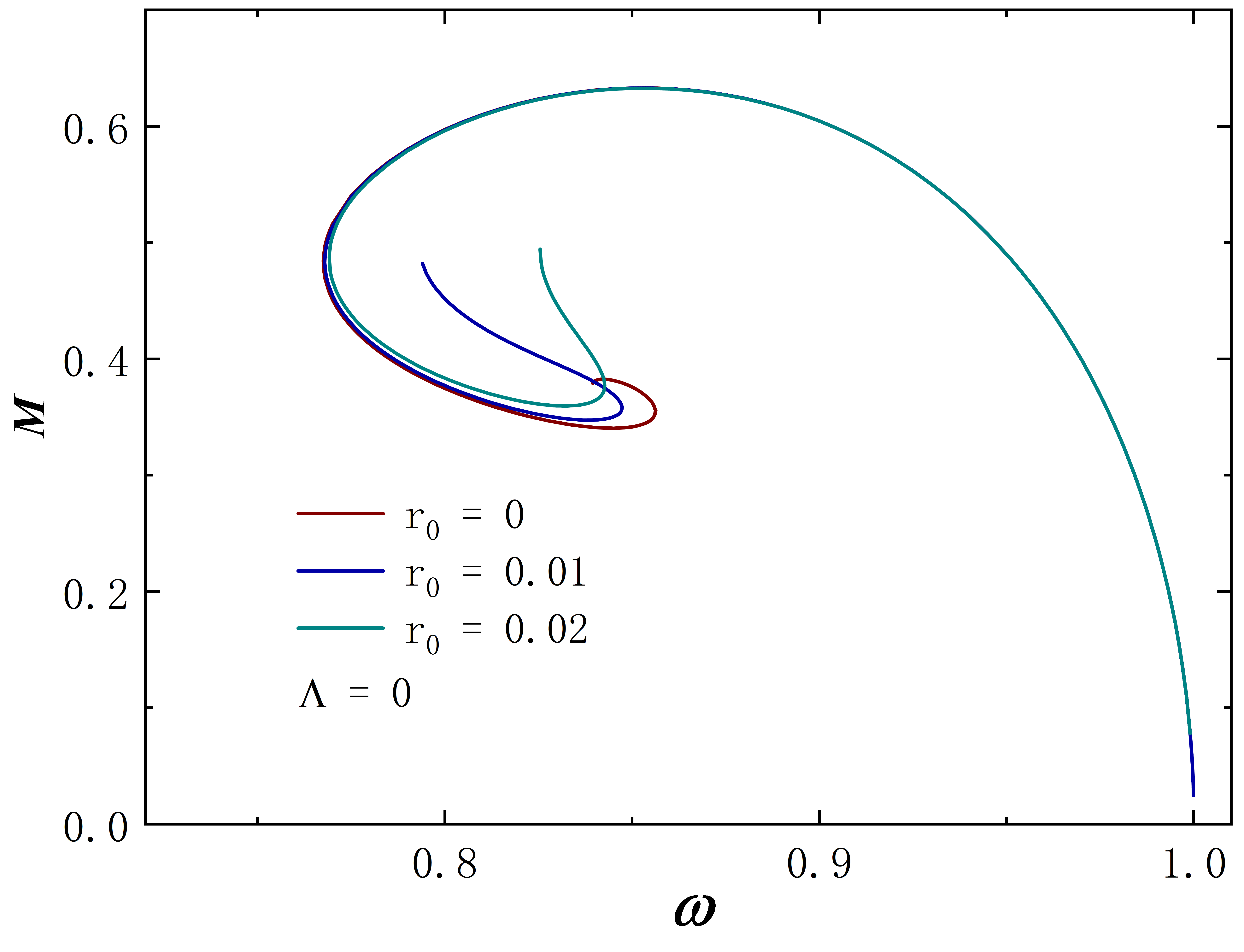
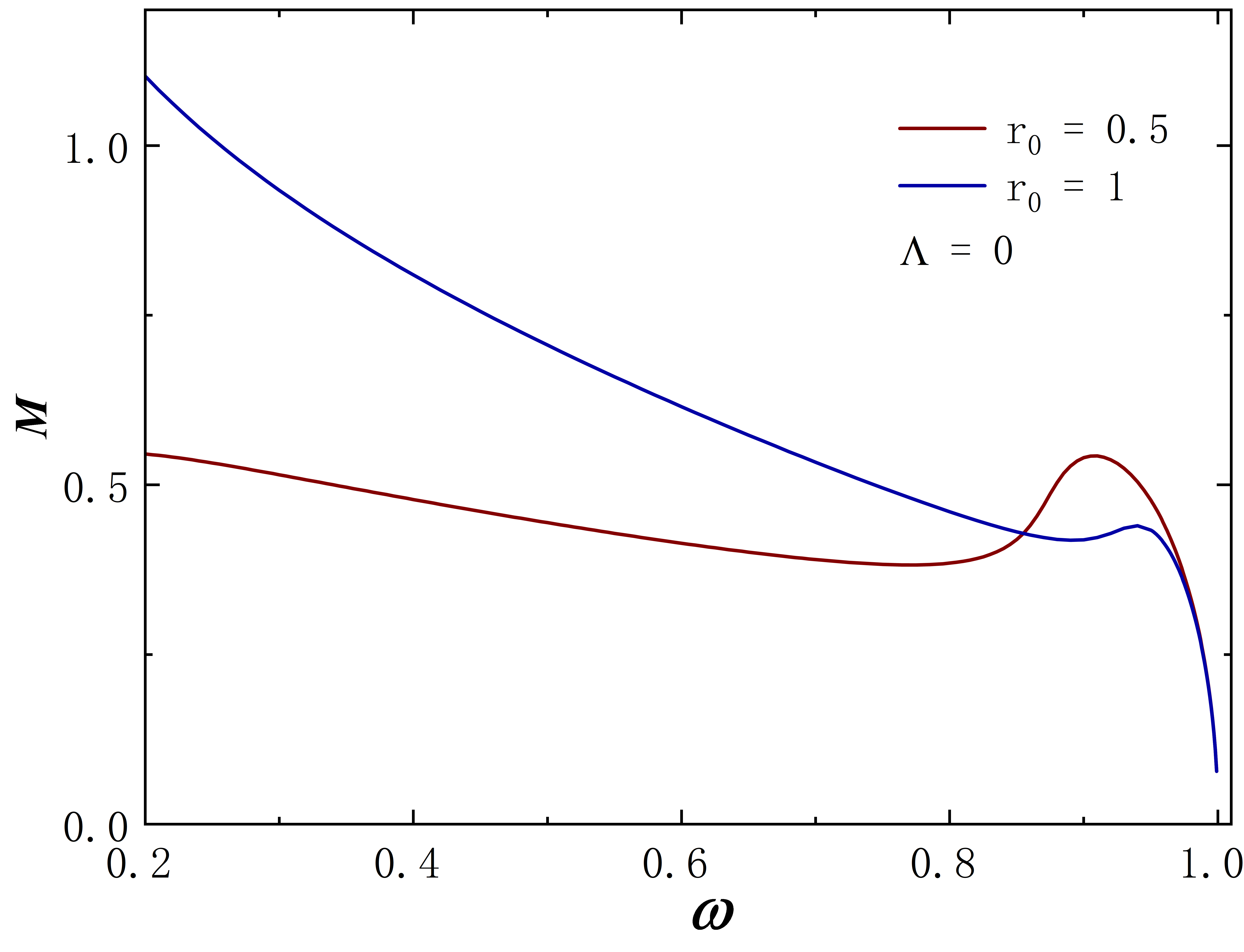
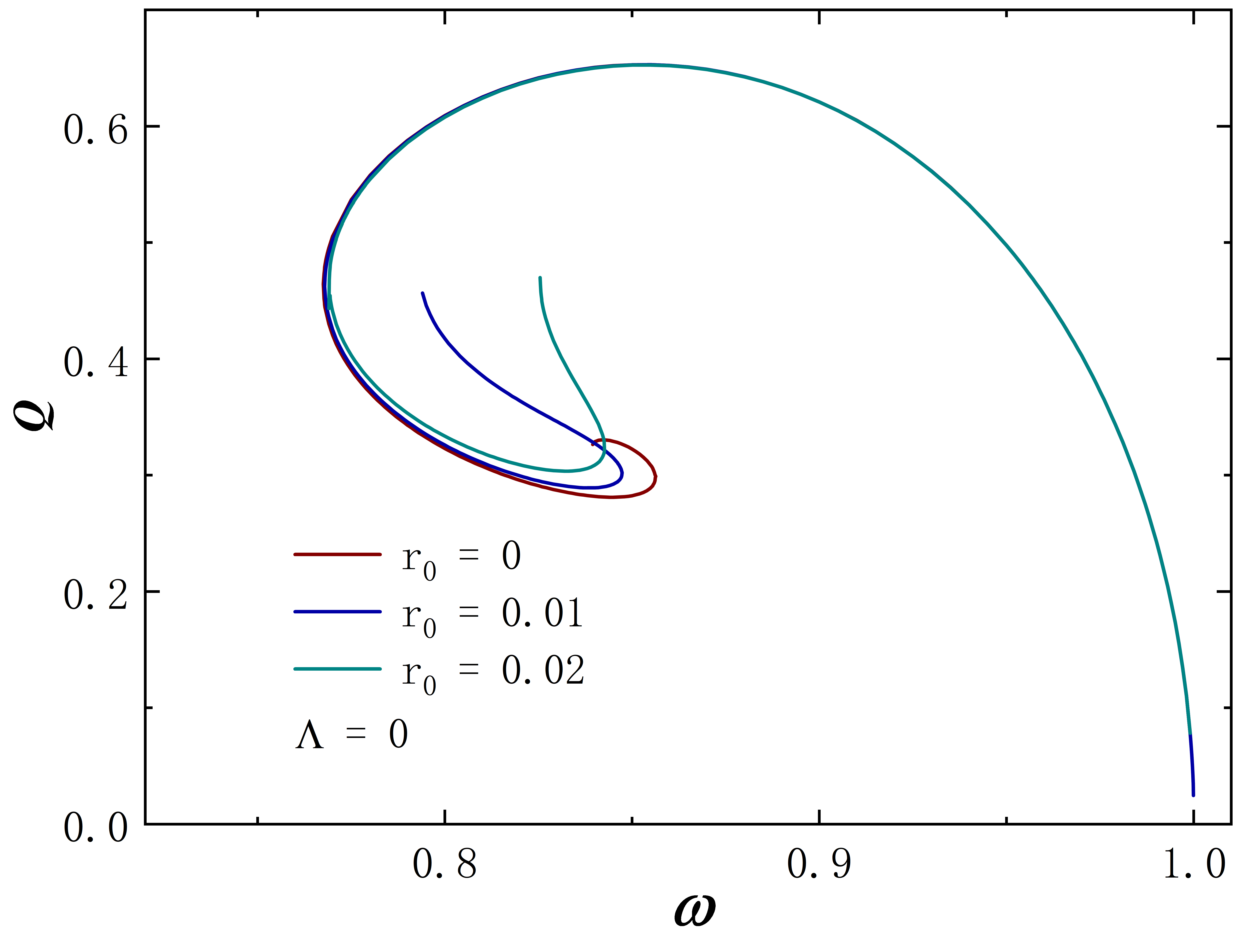
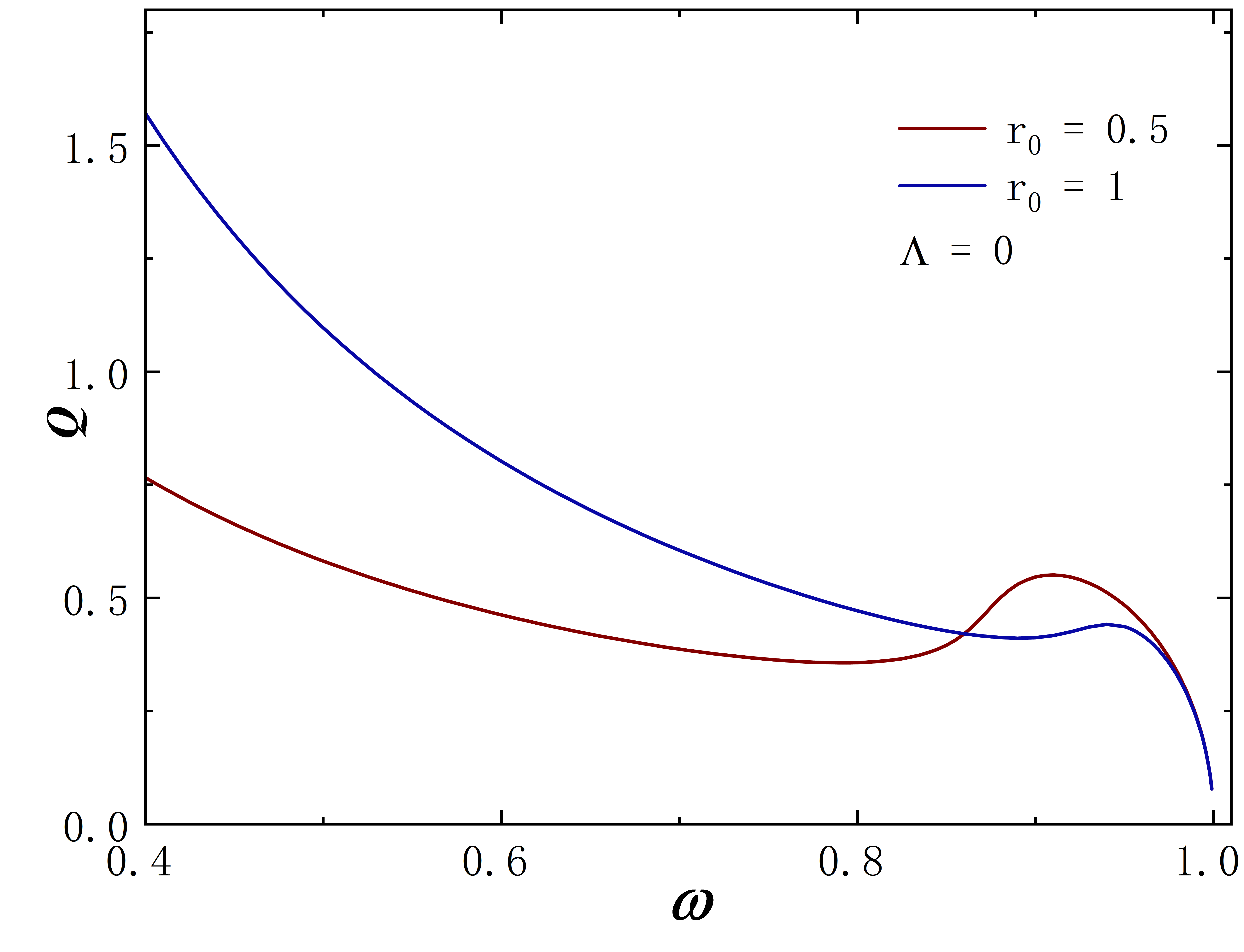
When the cosmological constant $\Lambda=0$, the solution degenerates to the static symmetric Ellis wormhole with a scalar field. At this juncture, we show the ADM mass $M$ and Noether charge $Q$ for this solution in Fig.1, and the numerical results are aligned with the Ding:2023syj . When $r_{0}$ is small, the solution will be limited in a tight range of $\omega$, and the curve shapes are just like the well-known spiral curve of Bonson stars. As $r_{0}$ increases, the spiral curve configuration gradually unfolds, eventually resulting in a single branch, such as the case of $r_{0}=1$. Notably, the mass $M$ and charge $Q$ at this time will sharply grow almost linearly as $\omega$ decreases, so we do not show the data when $\omega$ is very small. Further properties of this solution without cosmological constants will not be presented. Interested readers are encouraged to refer to the Ding:2023syj for additional details.

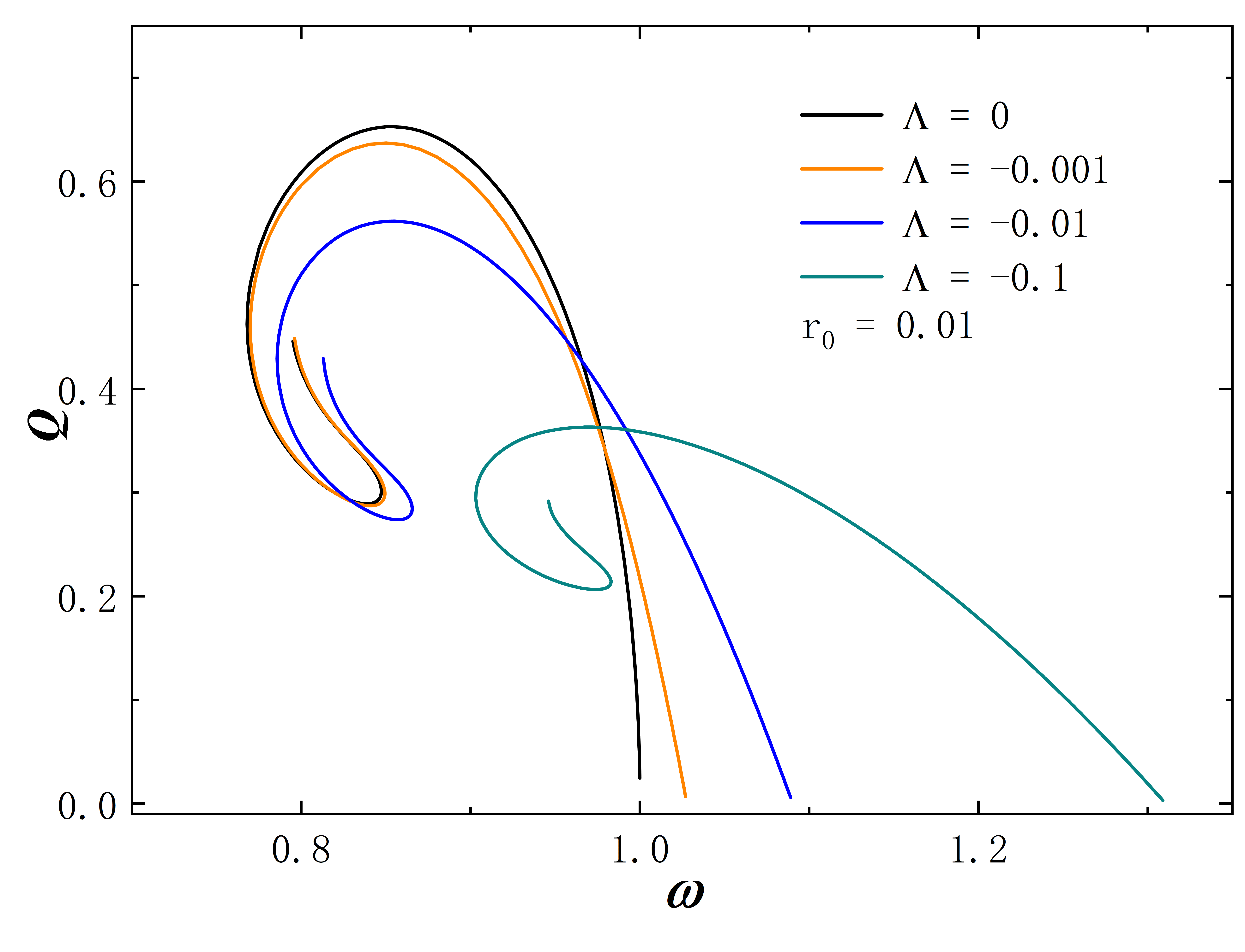
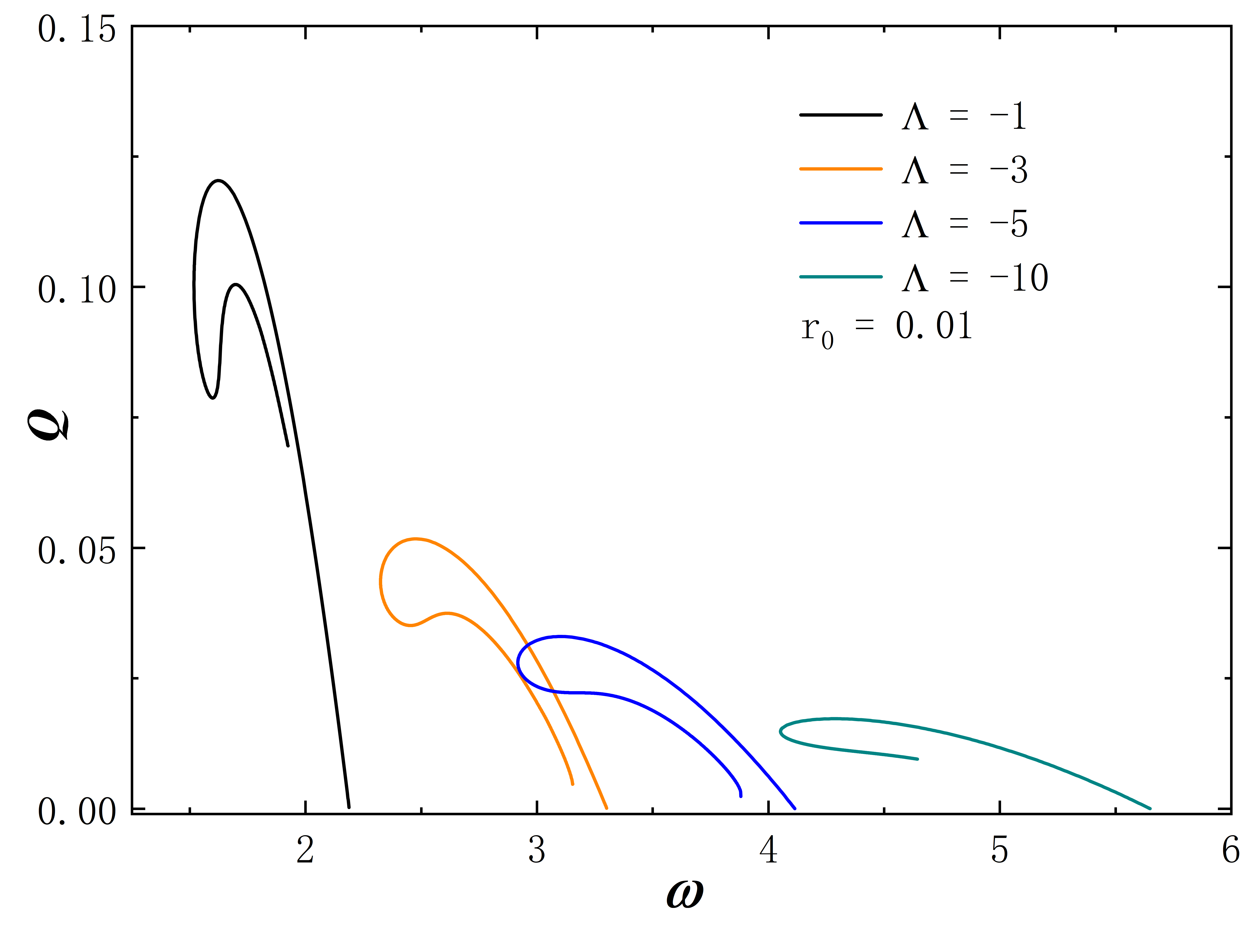
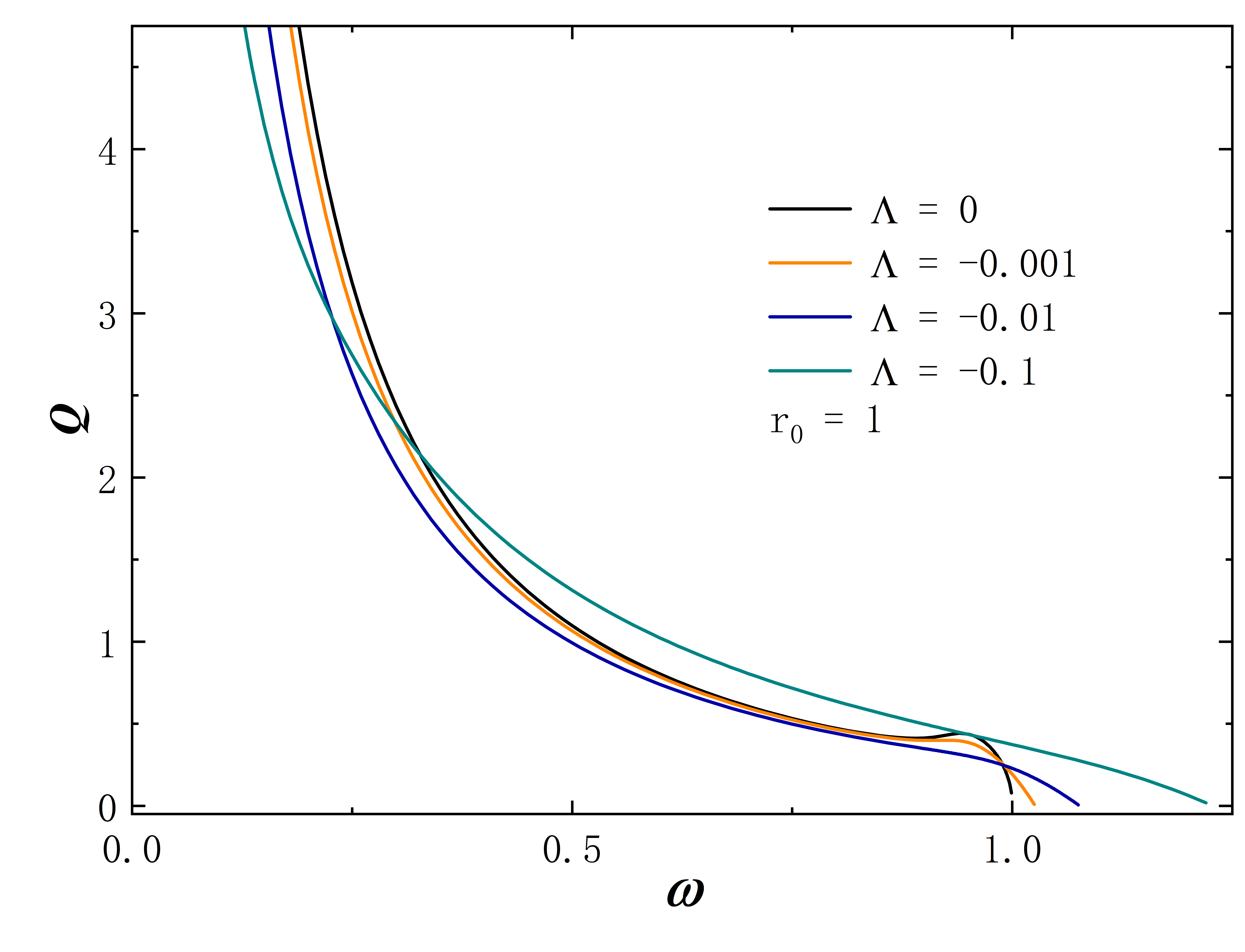
In the context of a negative cosmological constant, the odd terms in the metric $g_{tt}$ expansion vanish, implying that the ADM mass of the solution becomes zero. To investigate the solution’s properties, we study the functional relationship between the Noether charge $Q$ and frequency $\omega$ under varying cosmological constant $\Lambda$ for three distinct throat size $r_{0}$ groups, ranging from small to large.

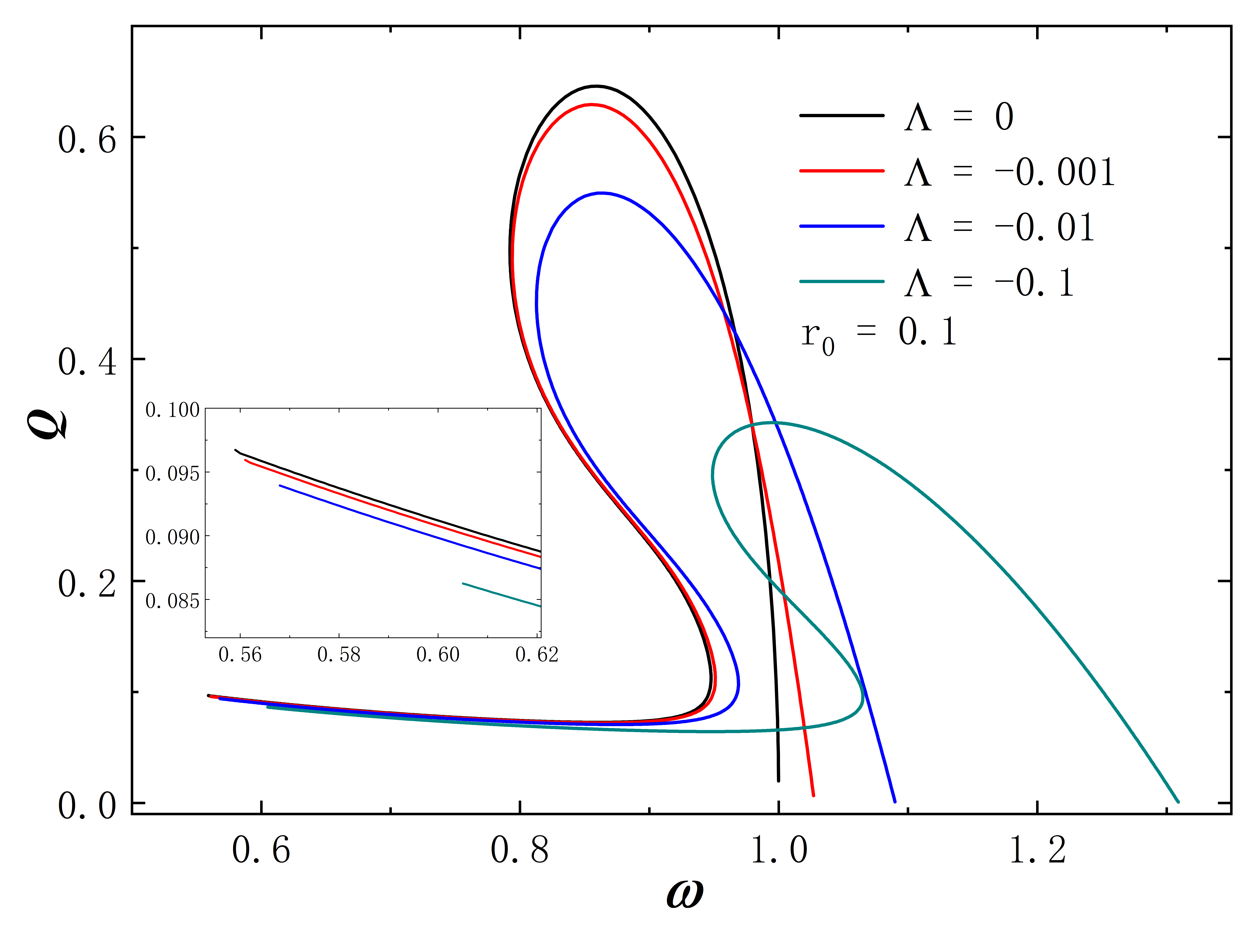
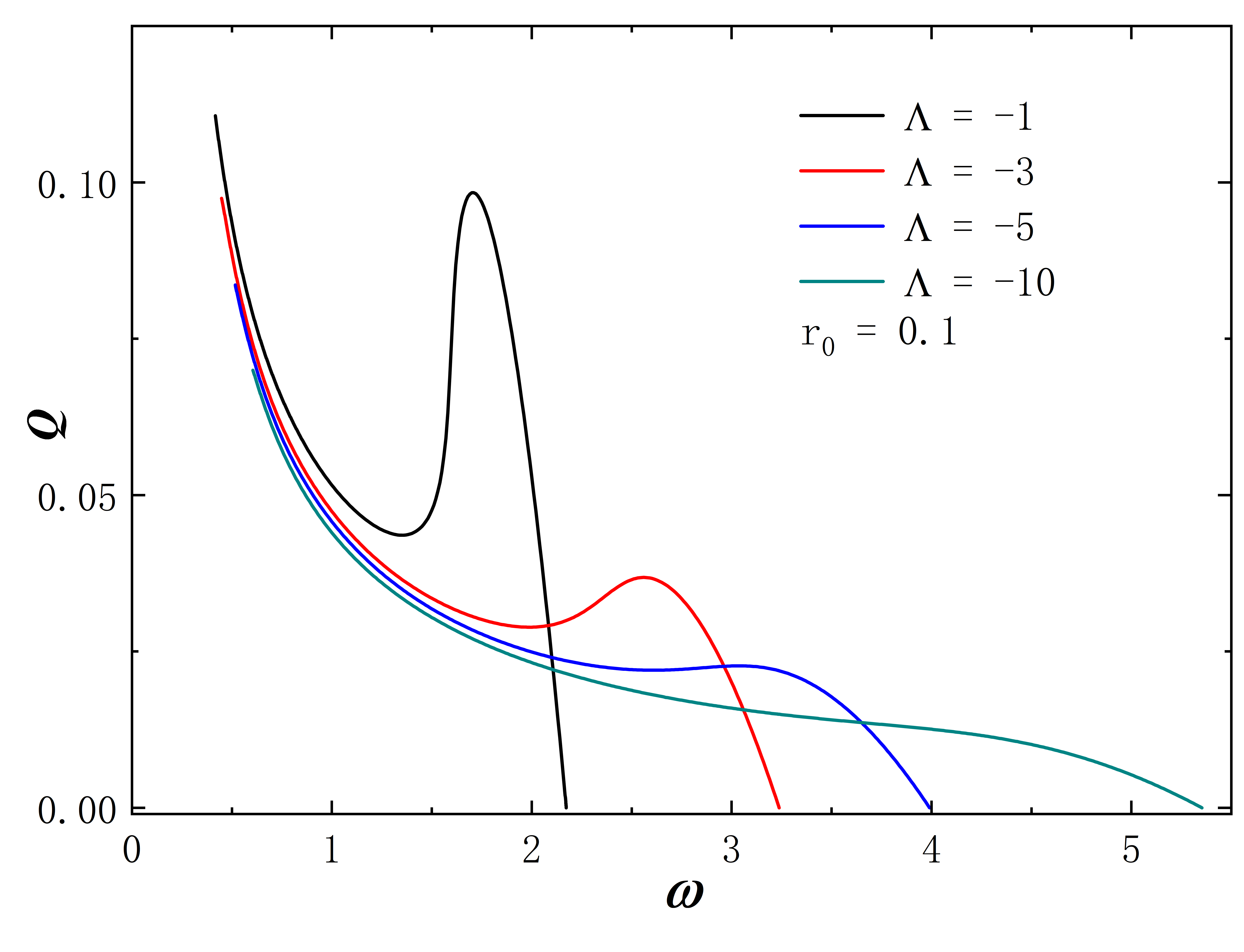
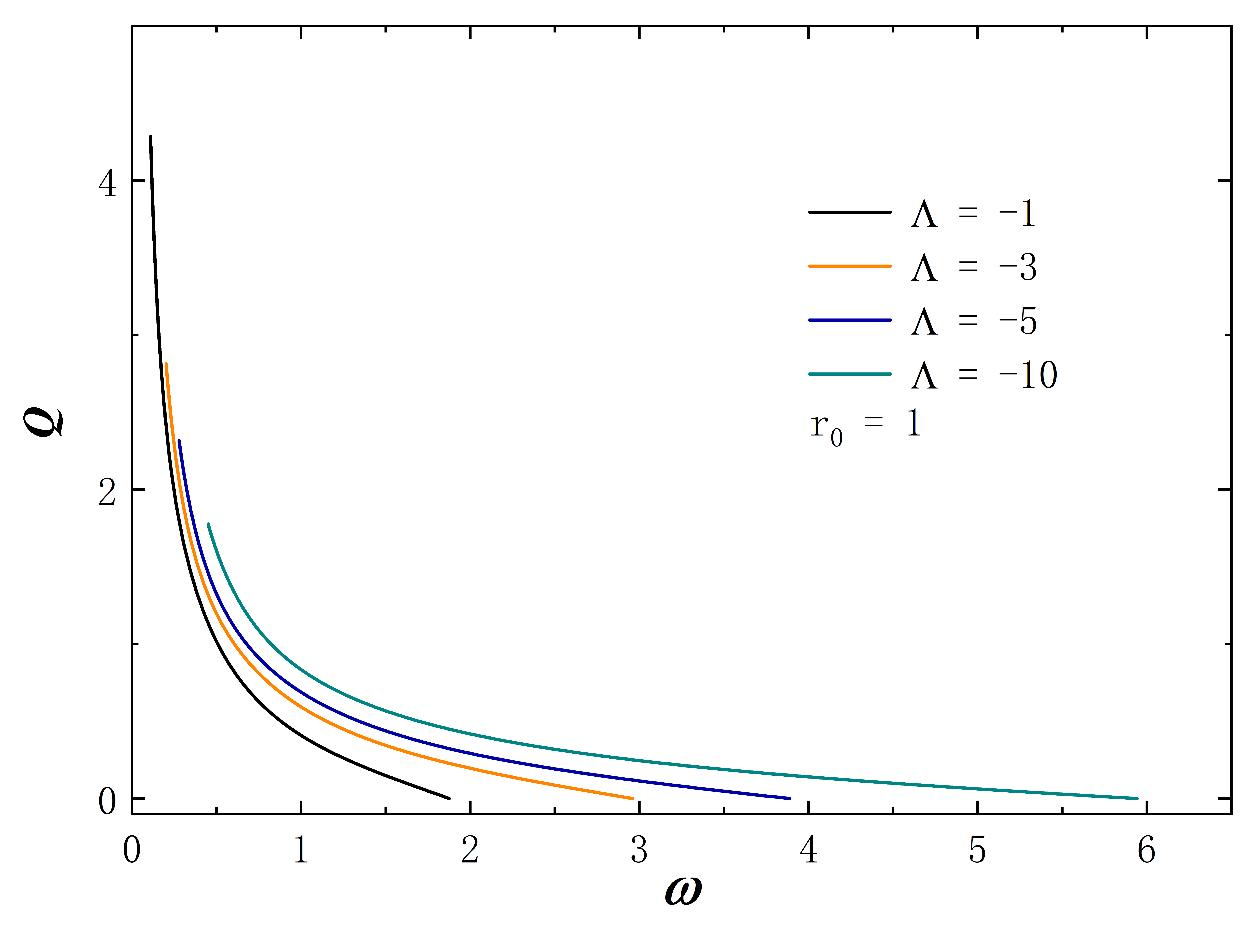
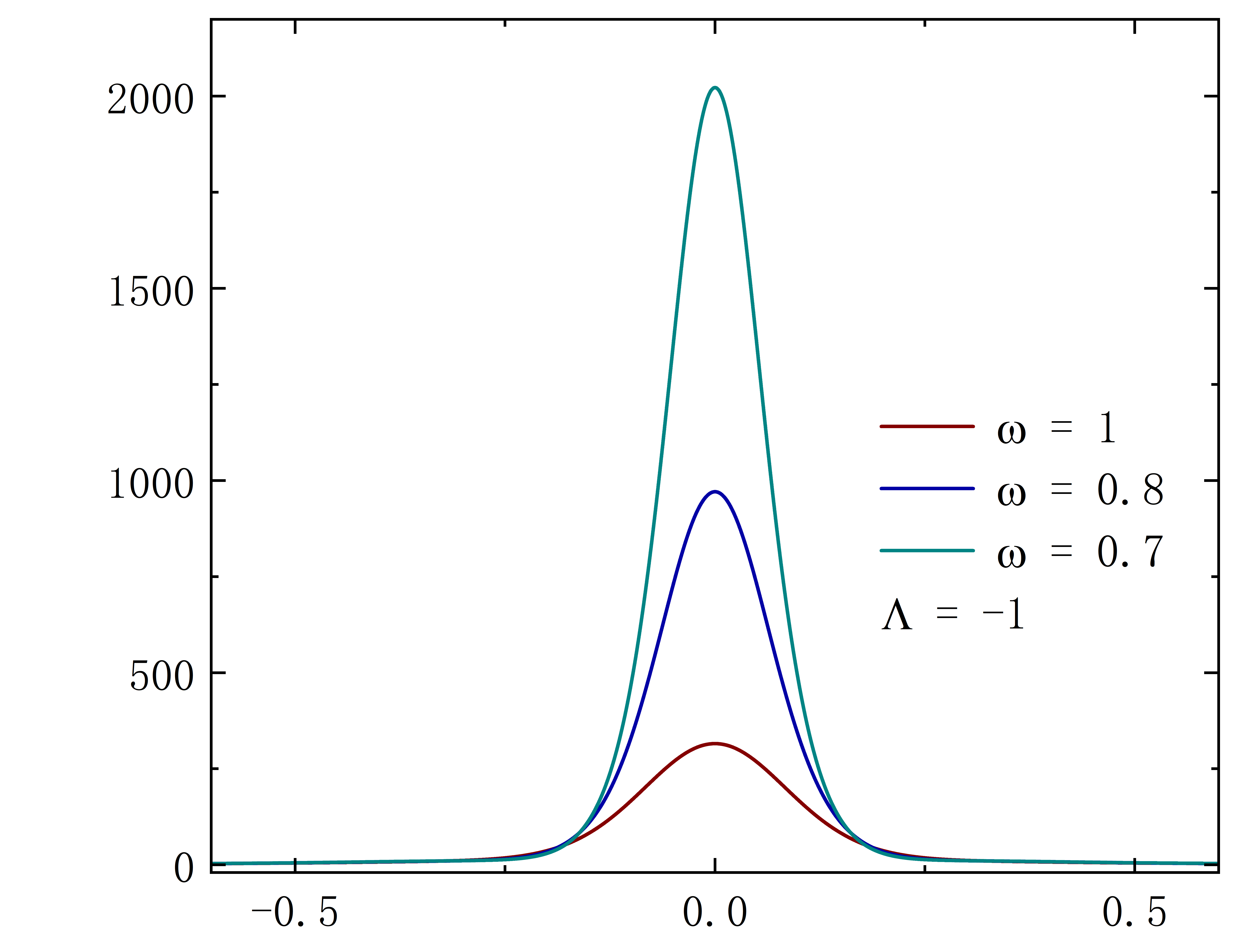
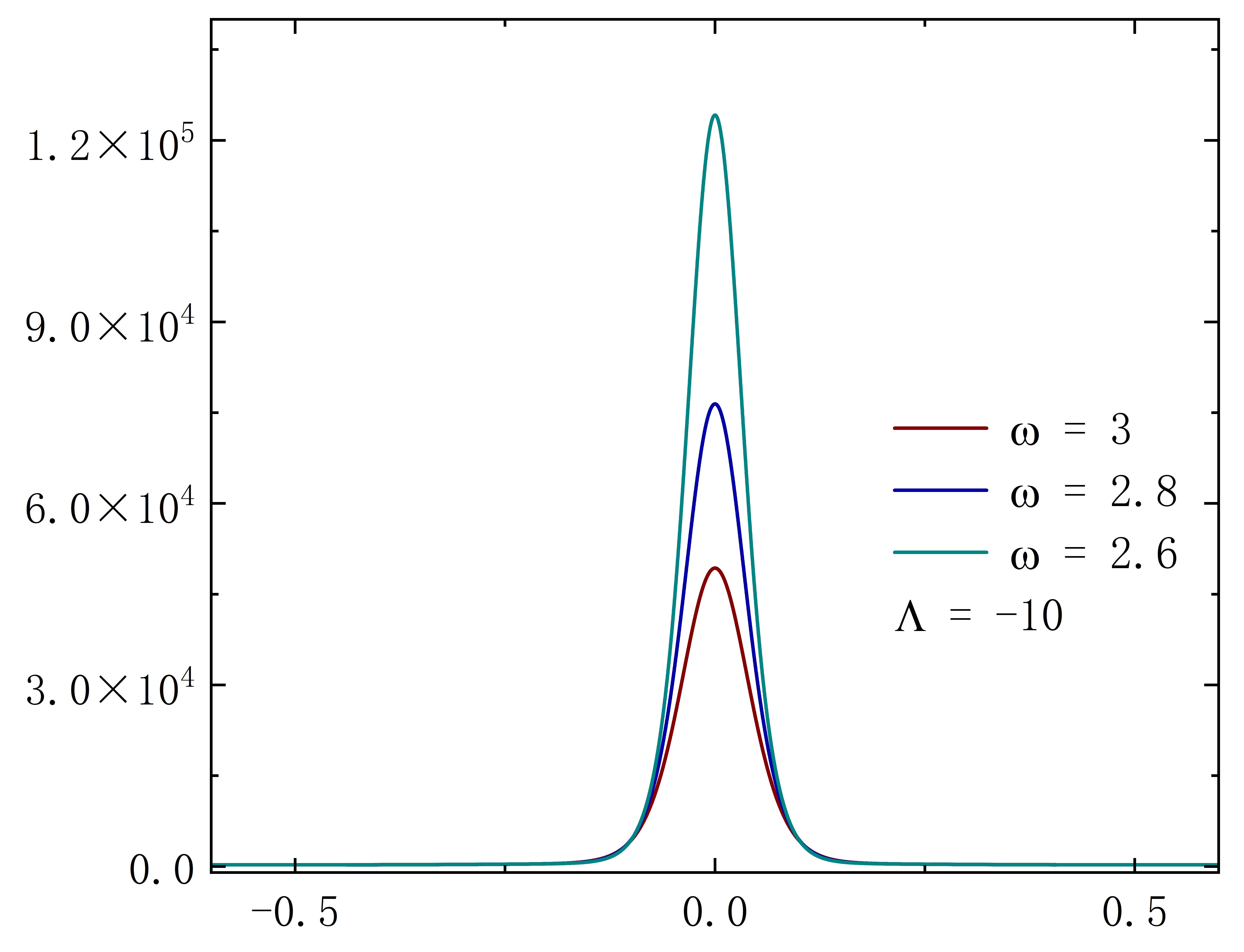
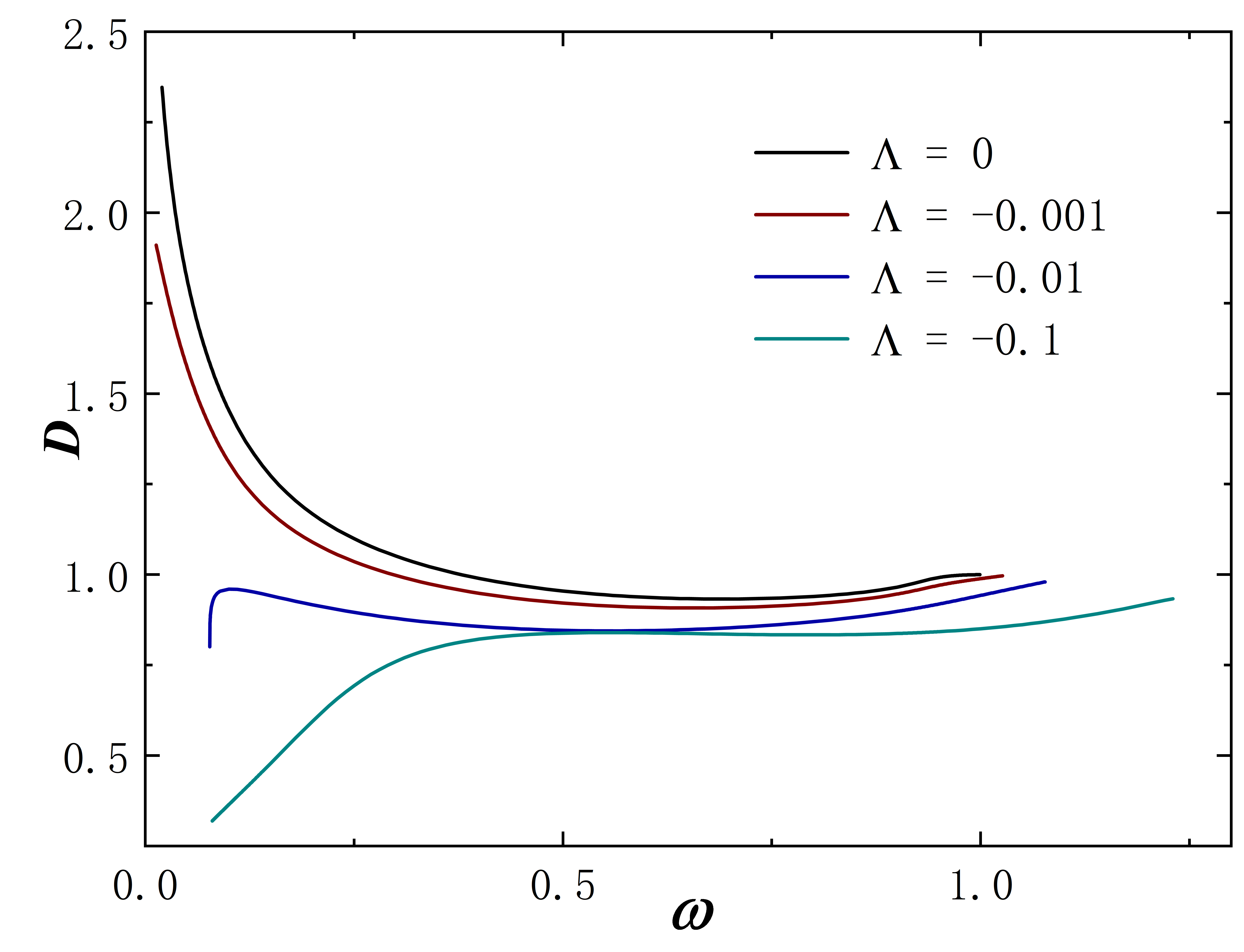
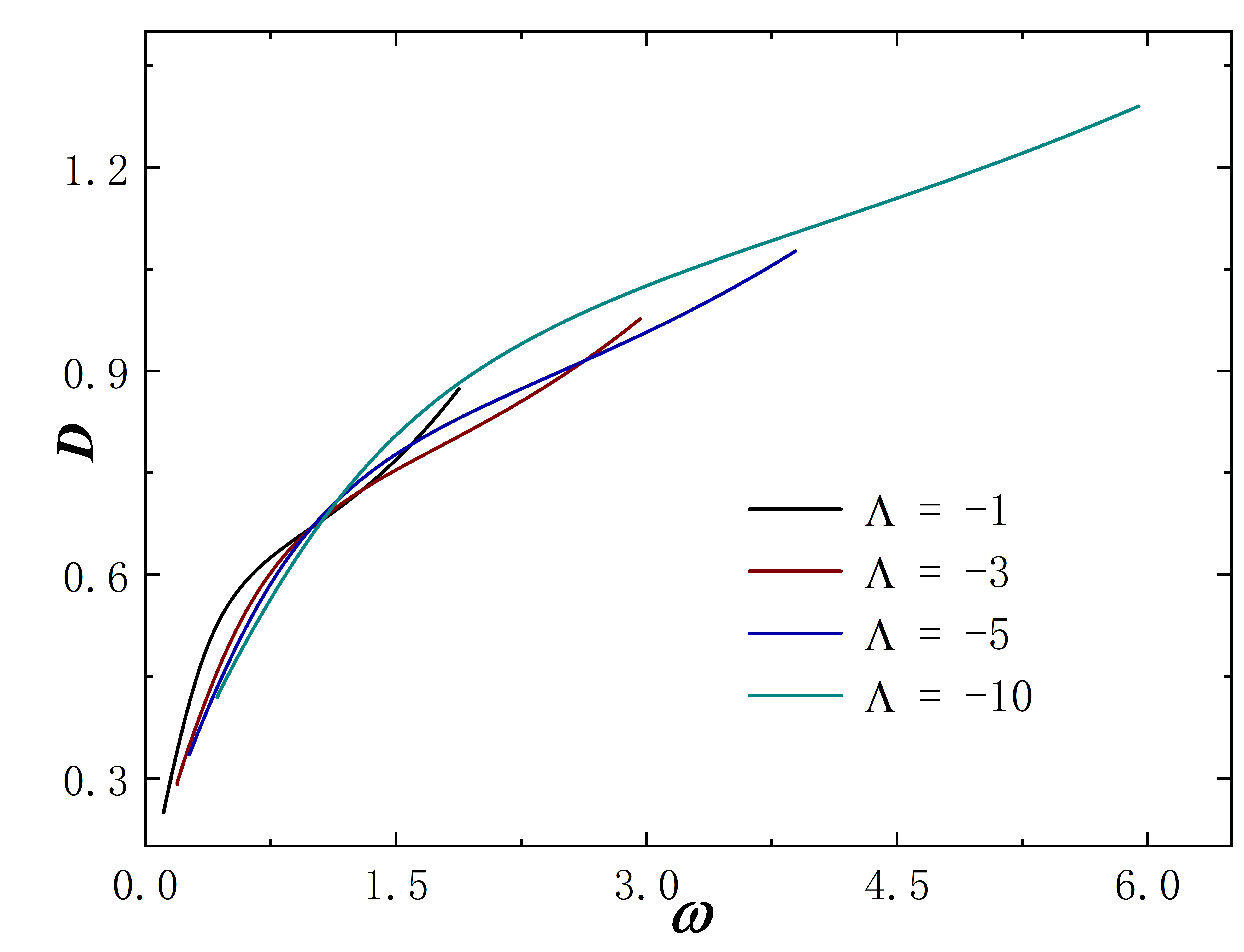
The Noether charge $Q$ as a function of frequency $\omega$ is shown in Fig.2. When the cosmological constant approaches zero, the solutions exhibit minimal deviation from $\Lambda=0$. This behavior is evident both in the curve shape and the magnitude of the Noether charge $Q$. As $\Lambda$ decreases further, gradual changes in solution properties become apparent. Specifically, for $r_{0}=0.01$, the reduction in the $\Lambda$ leads to fewer solution branches, the gradual unfolding of the corresponding spiral curve, and a decrease in the value of $Q$. The situation of $r_{0}=0.1$ exhibits similar behavior. However, for larger throat sizes, such as $r_{0}=1$, the situation diverges. At this time, the solution exhibits no branches regardless of the cosmological constant’s value and the Noether charge $Q$ does not exhibit an obvious monotonic change as $\Lambda$ decreases. Furthermore, the presence of a negative cosmological constant alters the solution’s existence domain, which is manifested in that as $\Lambda$ decreases, the frequency range of the solution expands and gradually shifts to the right.

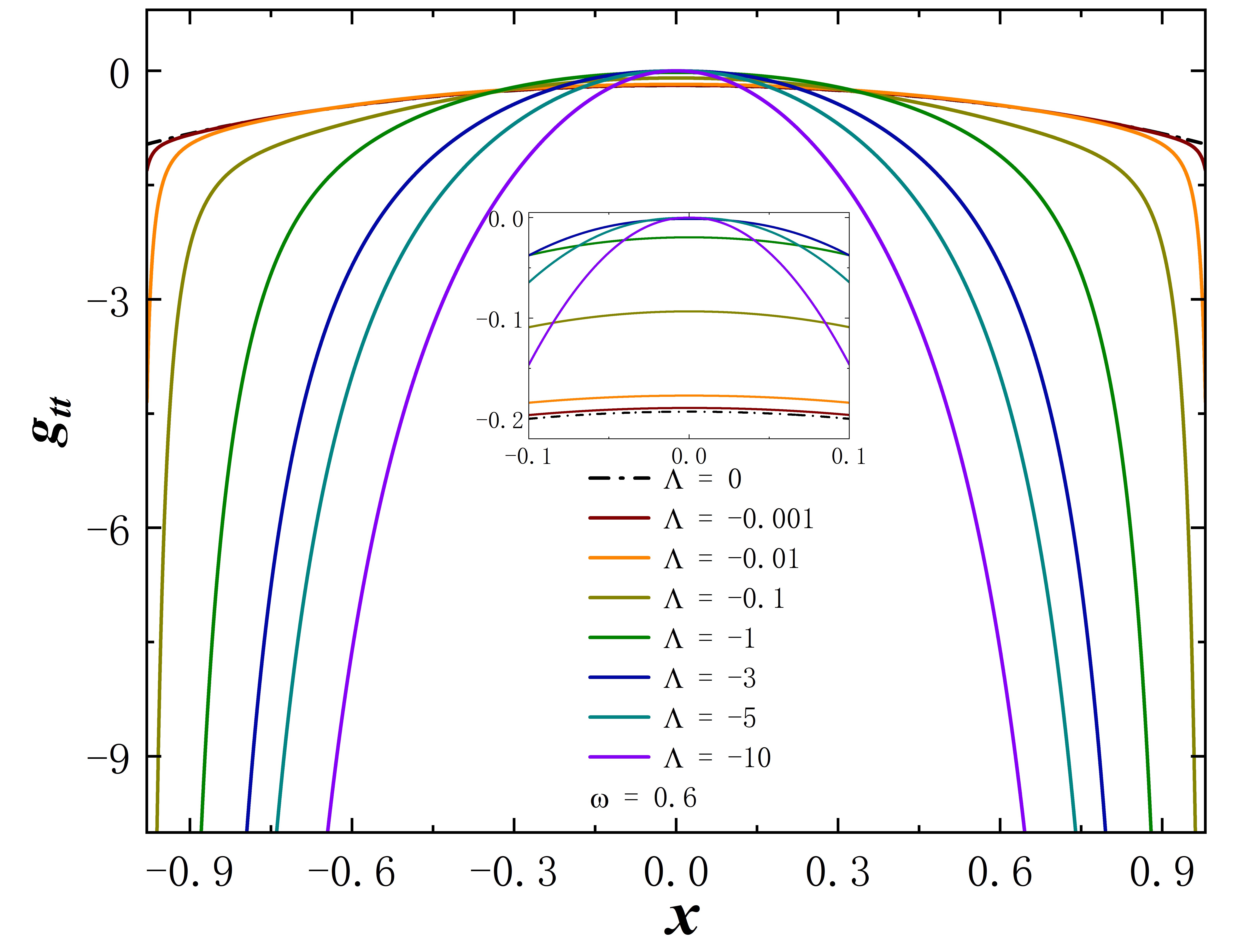
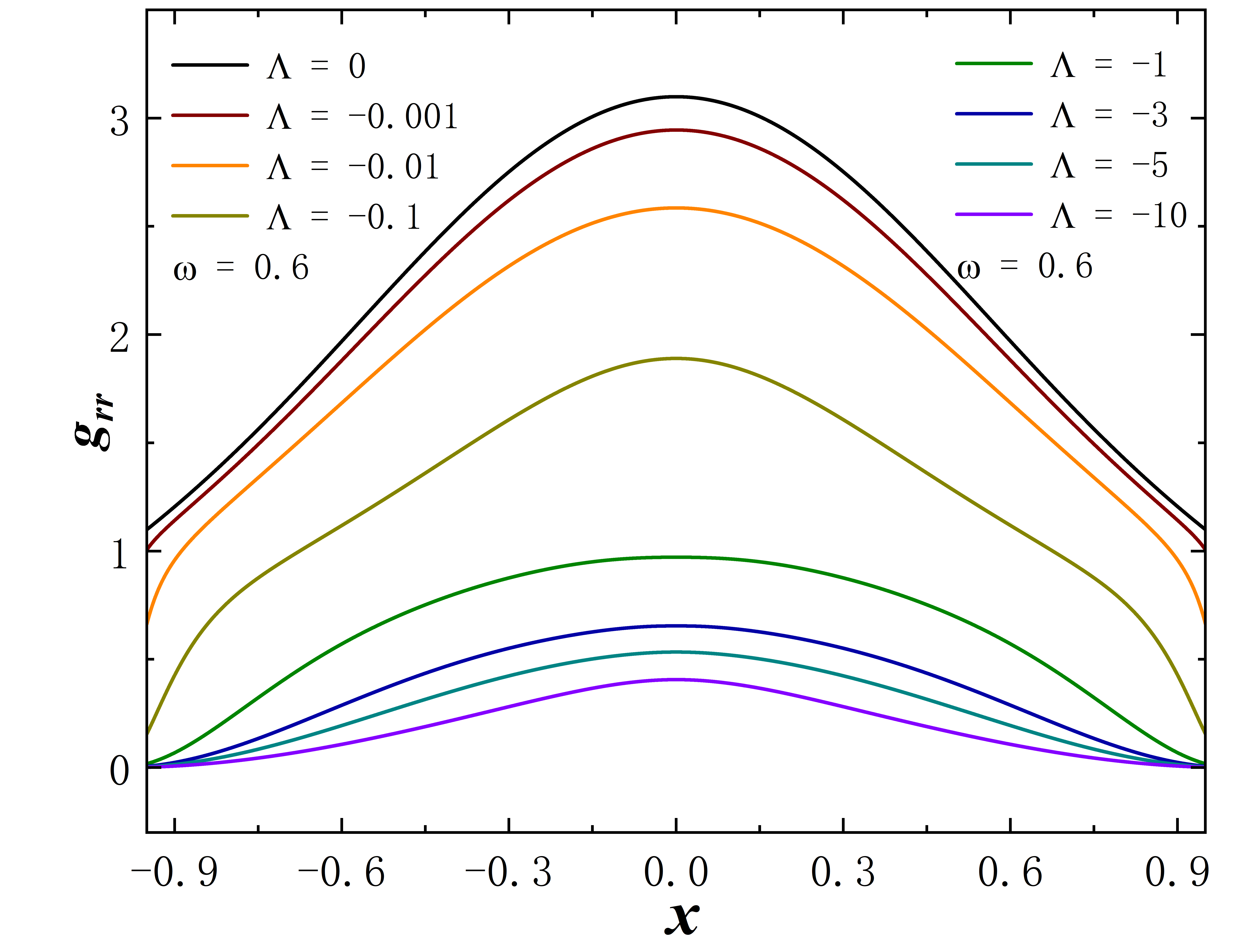
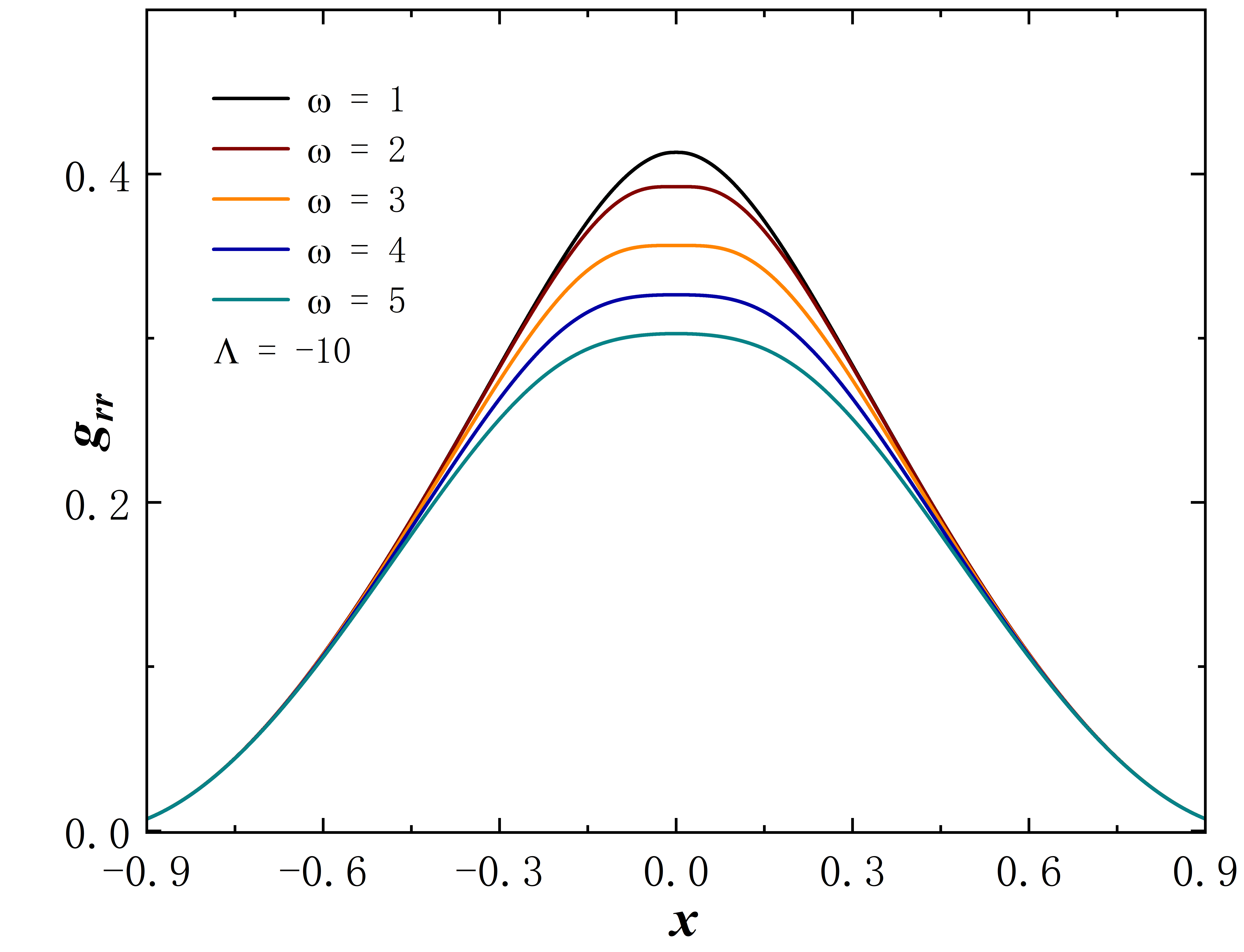
Without loss of generality, we set $r_{0}=1$ for all subsequent numerical results. The metric functions $g_{tt}$ and $g_{rr}$ characterize the spacetime properties of the solution, as depicted in Fig. 3. First, we fix the frequency $\omega$ at 0.6 and explore a range of different $\Lambda$ values, and the corresponding results are depicted in the figure on the first line. When $\Lambda$ takes 0, the solution aligns with the scenario described in Ding:2023syj . As $\Lambda$ decreases, the $g_{tt}$ value at $x=0$ gradually approaches 0. In terms of the Eq. (8) line element, this signifies the emergence of an approximate “event horizon”. In addition, taking the frequency to the right limit of the solution signifies the disappearance of the scalar field, causing the solution to degenerate back into the wormhole described in Blazquez-Salcedo:2020nsa . In the second row of the figure, the cosmological constant is fixed at -10, and we investigate the variation of the metric functions with frequency $\omega$. As $\omega$ gradually decreases (approaching the left limit of the solution), the value of $g_{tt}$ at $x=0$ once again approaches 0. The “extreme” behavior of the approximate “event horizon”, resulting from parameter variations in the solution, has been investigated in Hao:2023igi ; Su:2023xxk . This phenomenon bears a resemblance to the appearance of “one-way traversable wormholes” due to parameter changes in the metric within the context of “black-bounce” scenarios Simpson:2018tsi ; Lobo:2020ffi .

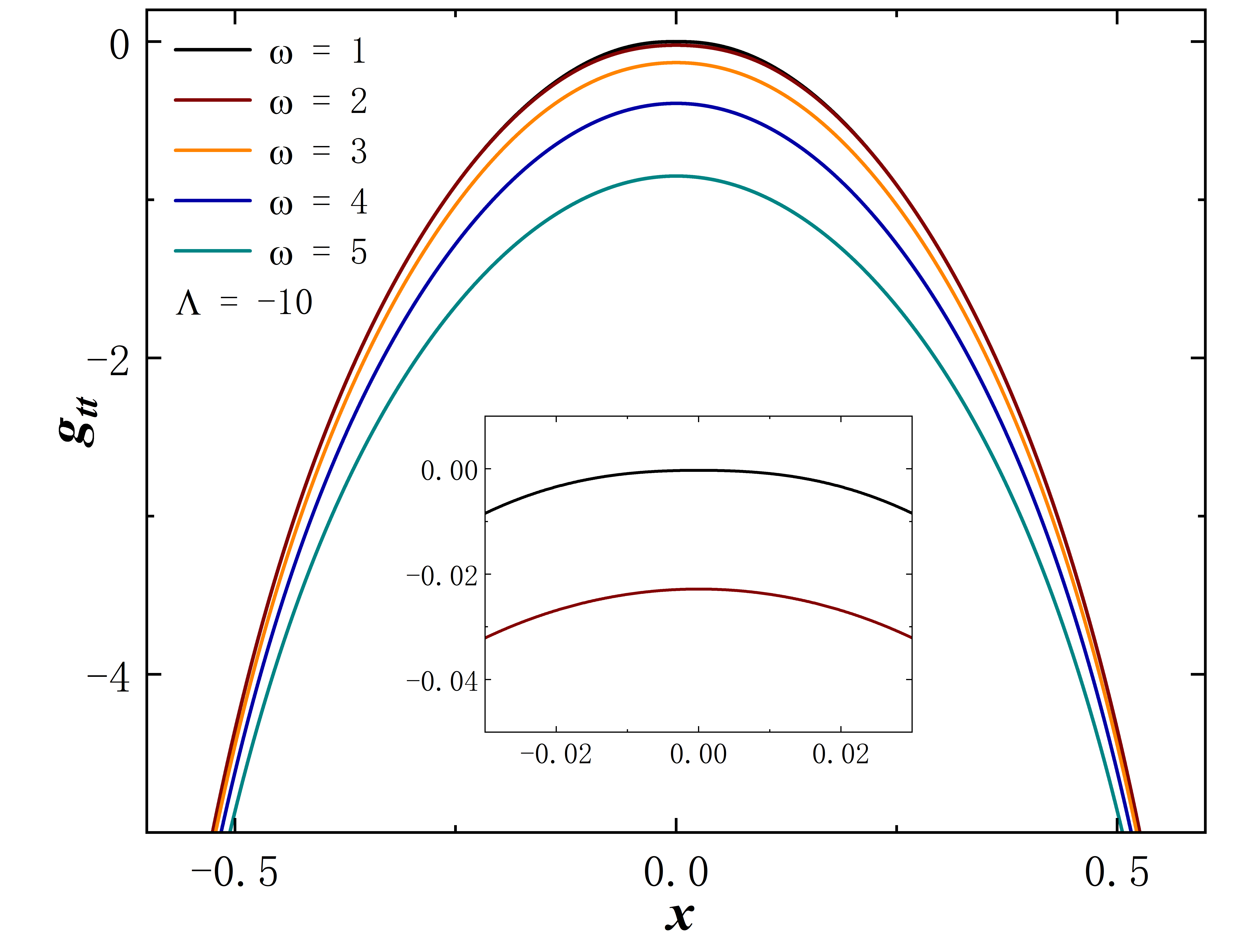
To better capture the behavior of the metric function $g_{tt}$ at the throat approaching zero, we employ Tab. 1 and Tab. 2 to denote the value of $g_{tt}$ at $x=0$ under decreasing cosmological constants or frequencies. It is evident that for sufficiently small values of $\Lambda$ or $\omega$, the minimum value of $g_{tt}$ can approach $10^{-7}$ or even smaller.

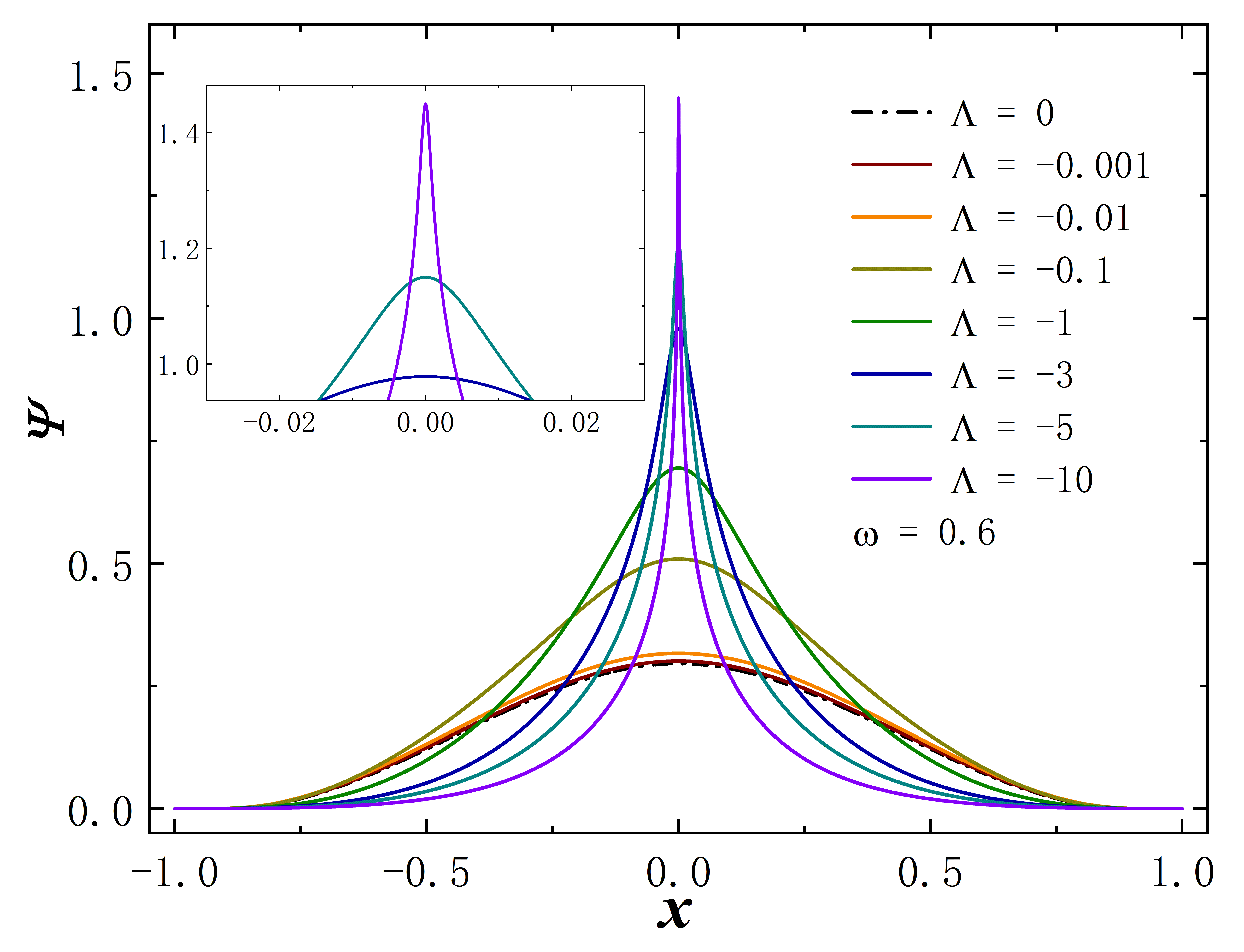
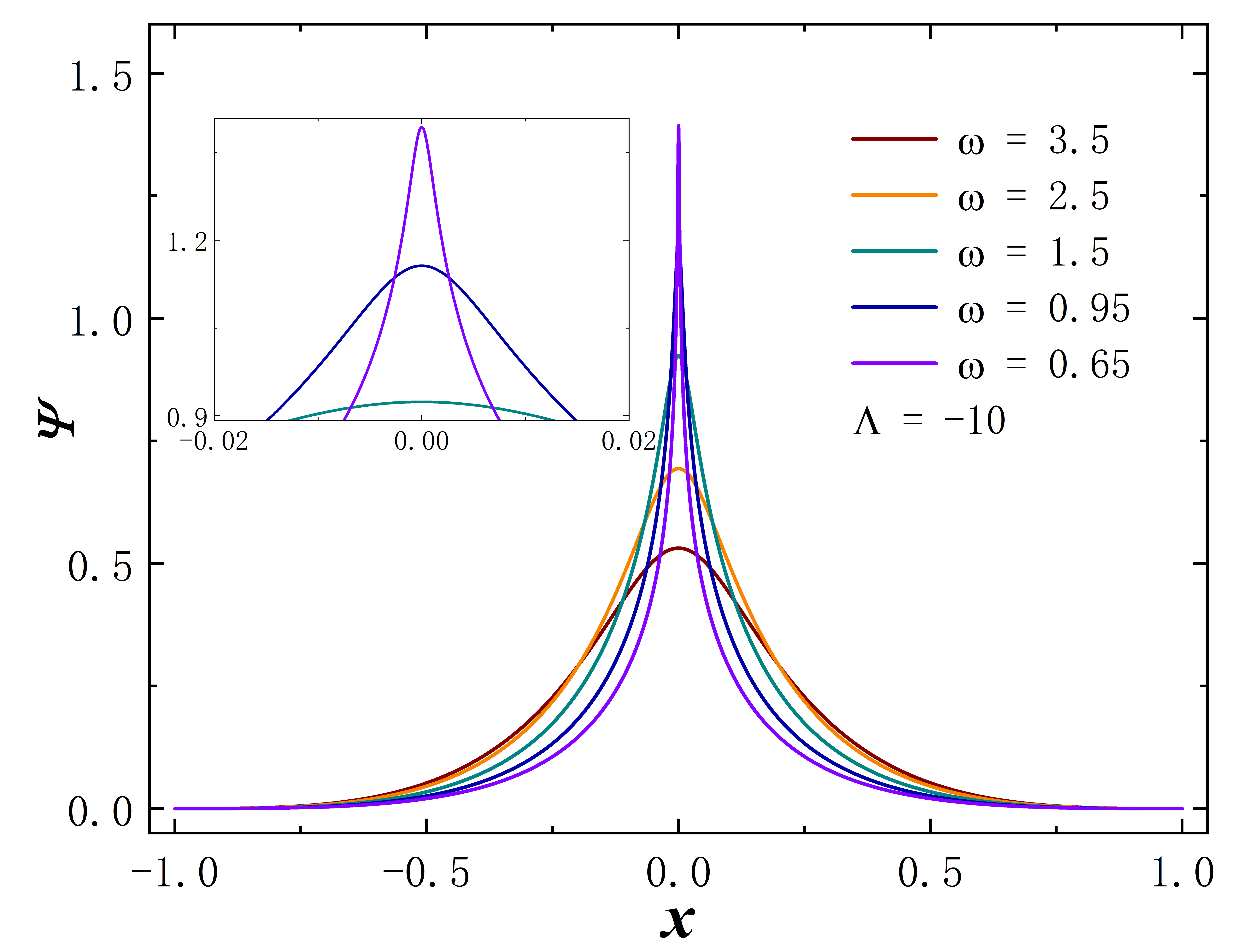
Given that this traversable wormhole solution is coupled with a scalar field, investigating the properties of the scalar field becomes highly relevant. Analogous to our previous approach, we fix the frequency at 0.6 or set the cosmological constant to -10. Subsequently, we explore the effects of varying $\Lambda$ or $\omega$ on the matter field within these two scenarios Fig. 4. Remarkably, we observe a recurring “extreme” behavior. As $\Lambda$ or $\omega$ decreases, the scalar field distribution near $x=0$ becomes highly concentrated, while the distribution in other regions of spacetime diminishes significantly. This property enables us to investigate the distribution of the Kretschmann scalar further. Fig. 5 illustrates the Kretschmann scalar distribution when $\Lambda$ remains constant while varying $\omega$. When $\Lambda$ remains constant, decreasing $\omega$ leads to an increased value of the Kretschmann scalar, concentrating it near $x=0$. Similarly, reducing $\Lambda$ at the same frequency $\omega$ produces a similar effect. The concentrated distribution of the matter field at the center of the wormhole, along with the nearly divergent Kretschmann scalar, suggests that within the parameter range where this “extreme” behavior occurs, the wormhole becomes untraversable.

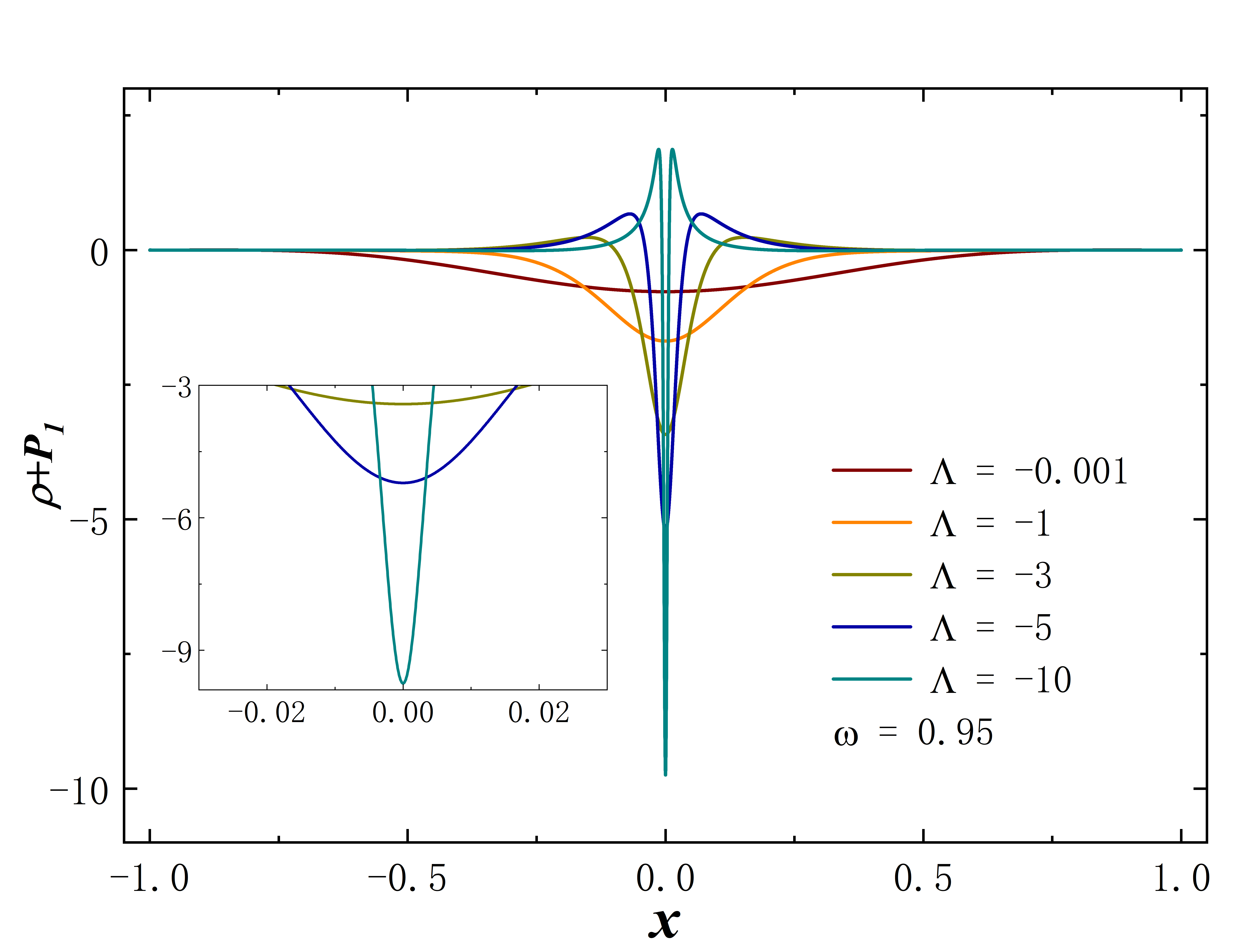
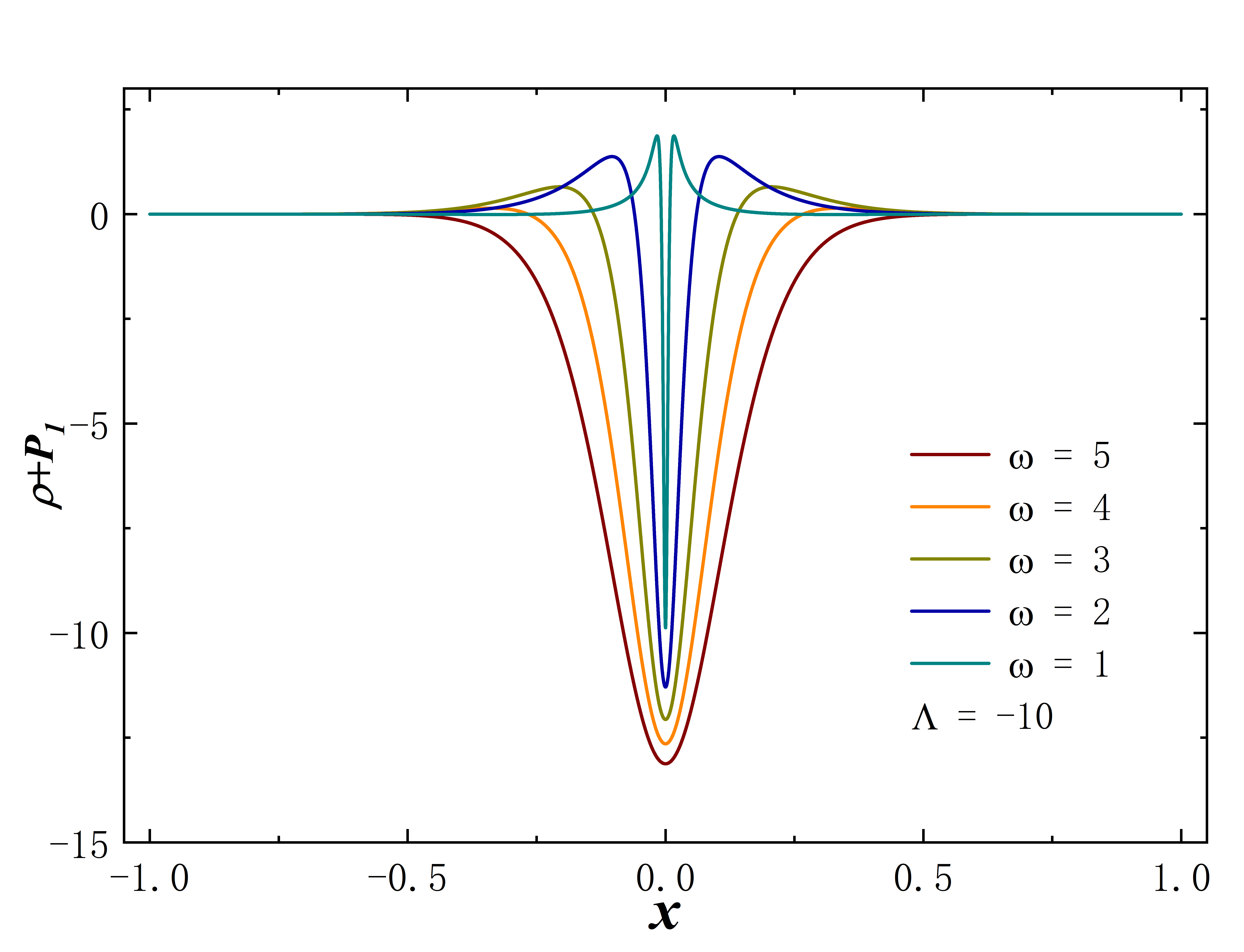
Ellis wormholes devoid of matter fields violate the null energy condition (NEC) due to the presence of a phantom field. However, what happens when a scalar field is coupled? We examine the sum of energy density $\rho$ and radial pressure $p_{1}$ in the context of varying the cosmological constant at a fixed frequency or altering the frequency while keeping the cosmological constant Fig. 6. While the violation of the null energy condition (NEC) persists at the wormhole throat, the degree of violation intensifies as $\Lambda$ decreases or $\omega$ increases. However, it is noteworthy that when the cosmological constant $\Lambda$ or frequency $\omega$ becomes small (specifically when $\Lambda\leq-3$ or $\omega\leq 4$ in the figure), two small regions symmetrically appear on both sides of the throat. Remarkably, within these spacetime regions, the NEC remains unviolated. This effect may arise from the contribution of a scalar field with positive energy density.

In the previous article, we defined the constant $\cal D$ to reflect the scalar charge of the phantom field and to test the accuracy of numerical calculations. Its value, fixed at $r_{0}=1$ as a function of frequency $\omega$, should be consistent at different positions, as shown in Fig. 7. Considering points at radial coordinates $x=0.01,0.5,0.6,0.9,-0.1,-0.2,-0.8$, the difference in $\cal D$ is smaller than $10^{-5}$. Analogously, if we concentrate solely on the value of $\cal D$ when the frequency is at its right limit (where the scalar field vanishes) in each scenario, the outcomes align with those observed in Blazquez-Salcedo:2020nsa . With decreasing $\Lambda$, the constant $\cal D$ at first decreases slightly to a minimum value and then increases as $\Lambda$ decreases further.

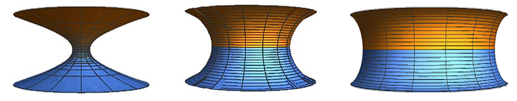
Finally, we study the geometric properties of the wormhole. We can make use of a geometrical embedding diagram by fixing $t$ and $\theta$. The resulting two-dimensional spatial hypersurface of the wormhole spacetime can then be embedded in a three-dimensional Euclidean space, where the embedding diagram can be used to visualize the wormhole geometry. This technique allows us to better understand the topology and properties of the wormhole solution.

The specific method is: we begin by constructing the embeddings of planes with $\theta=\pi/2$, and then use the cylindrical coordinates $(\rho,\varphi,z)$, the metric on this plane can be expressed by the following formula

	$\displaystyle ds^{2}$	$\displaystyle=\frac{p}{FN}dr^{2}+\frac{ph}{F}d\varphi^{2}\,$		(27)
		$\displaystyle=d\rho^{2}+dz^{2}+\rho^{2}d\varphi^{2}\,.$		(28)

Comparing the two equations above, we then obtain the expression for $\rho$ and $z$

$$\rho(r)=\sqrt{\frac{ph}{F}},\;\;\;\;\;\;\;\;\;\;z(r)=\pm\int\sqrt{\frac{p}{FN}-\left(\frac{d\rho}{dr}\right)^{2}}dr\;.$$

(29)

Here $\rho$ corresponds to the circumferential radius, which corresponds to the radius of a circle located in the equatorial plane and having a constant coordinate $r$. The function $\rho(r)$ has extreme points, where the first derivative is zero. When the second derivative of the extreme point is greater than zero, we call this point a throat, which corresponds to a minimal surface. When the second derivative of the extreme point is less than zero, we call this point an equator, which corresponds to a maximal surface.

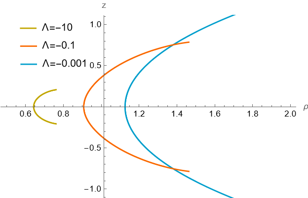
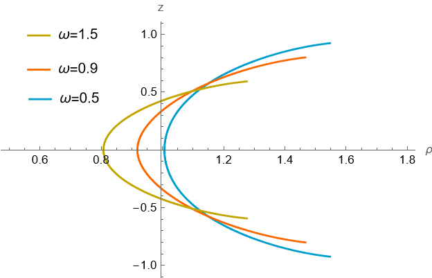
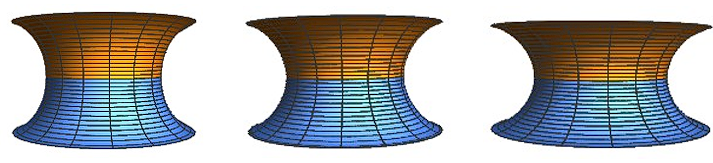
In Fig. 8, we present two sets of wormhole embedding diagrams. In the first row of figures, the frequency $\omega$ is fixed at 0.95, while the cosmological constants $\Lambda$ are varied as -0.001, -1, and -10. In the second row, the $\Lambda$ remains fixed at -1, and we explore three frequencies: 0.5, 0.9, and 1.5. Wormholes exhibit inherent symmetry and consistently possess a single throat without an equatorial plane. Decreasing the cosmological constant gradually widens the wormhole’s throat, whereas alterations in frequency have minimal impact on its geometric properties.

References

- (1) A. Einstein and N. Rosen, The Particle Problem in the General Theory of Relativity, Phys. Rev. 48 (1935), 73-77 doi:10.1103/PhysRev.48.73
- (2) M. D. Kruskal, Maximal extension of Schwarzschild metric, Phys. Rev. 119 (1960), 1743-1745 doi:10.1103/PhysRev.119.1743
- (3) R. W. Fuller and J. A. Wheeler, Causality and Multiply Connected Space-Time, Phys. Rev. 128 (1962), 919-929 doi:10.1103/PhysRev.128.919
- (4) C. W. Misner and J. A. Wheeler, Classical physics as geometry: Gravitation, electromagnetism, unquantized charge, and mass as properties of curved empty space, Annals Phys. 2 (1957), 525-603 doi:10.1016/0003-4916(57)90049-0
- (5) M. Visser, Traversable wormholes: Some simple examples, Phys. Rev. D 39 (1989), 3182-3184 doi:10.1103/PhysRevD.39.3182 [arXiv:0809.0907 [gr-qc]].
- (6) H. G. Ellis, Ether flow through a drainhole - a particle model in general relativity, J. Math. Phys. 14 (1973), 104-118 doi:10.1063/1.1666161
- (7) H. G. Ellis, THE EVOLVING, FLOWLESS DRAIN HOLE: A NONGRAVITATING PARTICLE MODEL IN GENERAL RELATIVITY THEORY, Gen. Rel. Grav. 10 (1979), 105-123 doi:10.1007/BF00756794
- (8) K. A. Bronnikov, Scalar-tensor theory and scalar charge, Acta Phys. Polon. B 4 (1973), 251-266
- (9) T. Kodama, General Relativistic Nonlinear Field: A Kink Solution in a Generalized Geometry, Phys. Rev. D 18 (1978), 3529-3534 doi:10.1103/PhysRevD.18.3529
- (10) M. S. Morris and K. S. Thorne, Wormholes in space-time and their use for interstellar travel: A tool for teaching general relativity, Am. J. Phys. 56 (1988), 395-412 doi:10.1119/1.15620
- (11) F. S. N. Lobo, Phys. Rev. D 71 (2005), 084011 doi:10.1103/PhysRevD.71.084011 [arXiv:gr-qc/0502099 [gr-qc]].
- (12) S. V. Sushkov, Phys. Rev. D 71 (2005), 043520 doi:10.1103/PhysRevD.71.043520 [arXiv:gr-qc/0502084 [gr-qc]].
- (13) F. S. N. Lobo, Phys. Rev. D 71 (2005), 124022 doi:10.1103/PhysRevD.71.124022 [arXiv:gr-qc/0506001 [gr-qc]].
- (14) K. A. Bronnikov, R. A. Konoplya and A. Zhidenko, Phys. Rev. D 86 (2012), 024028 doi:10.1103/PhysRevD.86.024028 [arXiv:1205.2224 [gr-qc]].
- (15) B. Kleihaus and J. Kunz, Phys. Rev. D 90 (2014), 121503 doi:10.1103/PhysRevD.90.121503 [arXiv:1409.1503 [gr-qc]].
- (16) D. I. Novikov, A. G. Doroshkevich, I. D. Novikov and A. A. Shatskiy, Astron. Rep. 53 (2009), 1079-1085 doi:10.1134/S1063772909120014 [arXiv:0911.4456 [gr-qc]].
- (17) K. A. Bronnikov, L. N. Lipatova, I. D. Novikov and A. A. Shatskiy, Grav. Cosmol. 19 (2013), 269-274 doi:10.1134/S0202289313040038 [arXiv:1312.6929 [gr-qc]].
- (18) F. Cremona, F. Pirotta and L. Pizzocchero, Gen. Rel. Grav. 51 (2019) no.1, 19 doi:10.1007/s10714-019-2501-x [arXiv:1805.02602 [gr-qc]].
- (19) H. Huang, H. Lü and J. Yang, Class. Quant. Grav. 39 (2022) no.18, 185009 doi:10.1088/1361-6382/ac8266 [arXiv:2010.00197 [gr-qc]].
- (20) K. A. Bronnikov and S. W. Kim, Possible wormholes in a brane world, Phys. Rev. D 67 (2003), 064027 doi:10.1103/PhysRevD.67.064027 [arXiv:gr-qc/0212112 [gr-qc]].
- (21) P. Kanti, B. Kleihaus and J. Kunz, Wormholes in Dilatonic Einstein-Gauss-Bonnet Theory Phys. Rev. Lett. 107 (2011), 271101 doi:10.1103/PhysRevLett.107.271101 [arXiv:1108.3003 [gr-qc]].
- (22) J. Maldacena and A. Milekhin, Humanly traversable wormholes Phys. Rev. D 103 (2021) no.6, 066007 doi:10.1103/PhysRevD.103.066007 [arXiv:2008.06618 [hep-th]].
- (23) J. L. Blázquez-Salcedo, C. Knoll and E. Radu, Traversable wormholes in Einstein-Dirac-Maxwell theory, Phys. Rev. Lett. 126 (2021) no.10, 101102 doi:10.1103/PhysRevLett.126.101102 [arXiv:2010.07317 [gr-qc]].
- (24) R. A. Konoplya and A. Zhidenko, Traversable Wormholes in General Relativity, Phys. Rev. Lett. 128 (2022) no.9, 091104 doi:10.1103/PhysRevLett.128.091104 [arXiv:2106.05034 [gr-qc]].
- (25) B. Kain, Einstein-Dirac-Maxwell wormholes in quantum field theory, [arXiv:2308.00049 [gr-qc]].
- (26) F. R. Klinkhamer, Defect Wormhole: A Traversable Wormhole Without Exotic Matter, Acta Phys. Polon. B 54 (2023) no.5, 5-A3 doi:10.5506/APhysPolB.54.5-A3 [arXiv:2301.00724 [gr-qc]].
- (27) J. M. Maldacena, Adv. Theor. Math. Phys. 2 (1998), 231-252 doi:10.4310/ATMP.1998.v2.n2.a1 [arXiv:hep-th/9711200 [hep-th]].
- (28) J. Maldacena and L. Susskind, Fortsch. Phys. 61 (2013), 781-811 doi:10.1002/prop.201300020 [arXiv:1306.0533 [hep-th]].
- (29) P. Gao, D. L. Jafferis and A. C. Wall, JHEP 12 (2017), 151 doi:10.1007/JHEP12(2017)151 [arXiv:1608.05687 [hep-th]].
- (30) J. Maldacena, D. Stanford and Z. Yang, Fortsch. Phys. 65 (2017) no.5, 1700034 doi:10.1002/prop.201700034 [arXiv:1704.05333 [hep-th]].
- (31) R. van Breukelen and K. Papadodimas, JHEP 08 (2018), 142 doi:10.1007/JHEP08(2018)142 [arXiv:1708.09370 [hep-th]].
- (32) J. Maldacena and X. L. Qi, [arXiv:1804.00491 [hep-th]].
- (33) D. C. Dai, D. Minic, D. Stojkovic and C. Fu, Phys. Rev. D 102 (2020) no.6, 066004 doi:10.1103/PhysRevD.102.066004 [arXiv:2002.08178 [hep-th]].
- (34) S. Bintanja, R. Espíndola, B. Freivogel and D. Nikolakopoulou, JHEP 10 (2021), 173 doi:10.1007/JHEP10(2021)173 [arXiv:2102.06628 [hep-th]].
- (35) A. Kundu, Eur. Phys. J. C 82 (2022) no.5, 447 doi:10.1140/epjc/s10052-022-10376-z [arXiv:2110.14958 [hep-th]].
- (36) B. Kain, Phys. Rev. Lett. 131 (2023) no.10, 101001 doi:10.1103/PhysRevLett.131.101001 [arXiv:2309.03314 [hep-th]].
- (37) J. P. S. Lemos, F. S. N. Lobo and S. Quinet de Oliveira, Phys. Rev. D 68 (2003), 064004 doi:10.1103/PhysRevD.68.064004 [arXiv:gr-qc/0302049 [gr-qc]].
- (38) J. P. S. Lemos and F. S. N. Lobo, Phys. Rev. D 69 (2004), 104007 doi:10.1103/PhysRevD.69.104007 [arXiv:gr-qc/0402099 [gr-qc]].
- (39) H. Maeda and M. Nozawa, Phys. Rev. D 78 (2008), 024005 doi:10.1103/PhysRevD.78.024005 [arXiv:0803.1704 [gr-qc]].
- (40) H. Maeda, Phys. Rev. D 86 (2012), 044016 doi:10.1103/PhysRevD.86.044016 [arXiv:1204.4472 [gr-qc]].
- (41) T. Wu, Phys. Rev. D 108 (2023) no.4, 044001 doi:10.1103/PhysRevD.108.044001 [arXiv:2209.02278 [gr-qc]].
- (42) M. Nozawa, Phys. Rev. D 103 (2021) no.2, 024005 doi:10.1103/PhysRevD.103.024005 [arXiv:2010.07561 [gr-qc]].
- (43) A. Anabalón and J. Oliva, JHEP 04 (2019), 106 doi:10.1007/JHEP04(2019)106 [arXiv:1811.03497 [hep-th]].
- (44) R. V. Korolev and S. V. Sushkov, Phys. Rev. D 90 (2014), 124025 doi:10.1103/PhysRevD.90.124025 [arXiv:1408.1235 [gr-qc]].
- (45) G. Franciolini, L. Hui, R. Penco, L. Santoni and E. Trincherini, JHEP 01 (2019), 221 doi:10.1007/JHEP01(2019)221 [arXiv:1811.05481 [hep-th]].
- (46) N. Chatzifotis, G. Koutsoumbas and E. Papantonopoulos, Phys. Rev. D 104 (2021) no.2, 024039 doi:10.1103/PhysRevD.104.024039 [arXiv:2011.08770 [gr-qc]].
- (47) J. L. Blázquez-Salcedo, X. Y. Chew, J. Kunz and D. H. Yeom, Eur. Phys. J. C 81 (2021) no.9, 858 doi:10.1140/epjc/s10052-021-09645-0 [arXiv:2012.06213 [gr-qc]].
- (48) J. A. Wheeler, Phys. Rev. 97 (1955), 511-536 doi:10.1103/PhysRev.97.511
- (49) E. A. Power and J. A. Wheeler, Rev. Mod. Phys. 29 (1957), 480-495 doi:10.1103/RevModPhys.29.480
- (50) D. J. Kaup, Phys. Rev. 172 (1968), 1331-1342 doi:10.1103/PhysRev.172.1331
- (51) R. Ruffini and S. Bonazzola, Phys. Rev. 187 (1969), 1767-1783 doi:10.1103/PhysRev.187.1767
- (52) F. E. Schunck and E. W. Mielke, Phys. Lett. A 249 (1998), 389-394 doi:10.1016/S0375-9601(98)00778-6
- (53) S. Yoshida and Y. Eriguchi, Phys. Rev. D 56 (1997), 762-771 doi:10.1103/PhysRevD.56.762
- (54) A. Bernal, J. Barranco, D. Alic and C. Palenzuela, Phys. Rev. D 81 (2010), 044031 doi:10.1103/PhysRevD.81.044031 [arXiv:0908.2435 [gr-qc]].
- (55) L. G. Collodel, B. Kleihaus and J. Kunz, Phys. Rev. D 96 (2017) no.8, 084066 doi:10.1103/PhysRevD.96.084066 [arXiv:1708.02057 [gr-qc]].
- (56) Y. Q. Wang, Y. X. Liu and S. W. Wei, Phys. Rev. D 99 (2019) no.6, 064036 doi:10.1103/PhysRevD.99.064036 [arXiv:1811.08795 [gr-qc]].
- (57) C. A. R. Herdeiro, J. Kunz, I. Perapechka, E. Radu and Y. Shnir, Phys. Rev. D 103 (2021) no.6, 065009 doi:10.1103/PhysRevD.103.065009 [arXiv:2101.06442 [gr-qc]].
- (58) D. Astefanesei and E. Radu, Nucl. Phys. B 665 (2003), 594-622 doi:10.1016/S0550-3213(03)00482-6 [arXiv:gr-qc/0309131 [gr-qc]].
- (59) A. Buchel, S. L. Liebling and L. Lehner, Phys. Rev. D 87 (2013) no.12, 123006 doi:10.1103/PhysRevD.87.123006 [arXiv:1304.4166 [gr-qc]].
- (60) M. Maliborski and A. Rostworowski, [arXiv:1307.2875 [gr-qc]].
- (61) G. Fodor, P. Forgács and P. Grandclément, Phys. Rev. D 92 (2015) no.2, 025036 doi:10.1103/PhysRevD.92.025036 [arXiv:1503.07746 [gr-qc]].
- (62) Y. Brihaye, B. Hartmann and S. Tojiev, Class. Quant. Grav. 30 (2013), 115009 doi:10.1088/0264-9381/30/11/115009 [arXiv:1301.2452 [hep-th]].
- (63) H. S. Liu, H. Lu and Y. Pang, Phys. Rev. D 102 (2020) no.12, 126008 doi:10.1103/PhysRevD.102.126008 [arXiv:2007.15017 [hep-th]].
- (64) V. Dzhunushaliev, V. Folomeev, C. Hoffmann, B. Kleihaus and J. Kunz, Phys. Rev. D 90 (2014) no.12, 124038 doi:10.1103/PhysRevD.90.124038 [arXiv:1409.6978 [gr-qc]].
- (65) C. Hoffmann, T. Ioannidou, S. Kahlen, B. Kleihaus and J. Kunz, Phys. Rev. D 95 (2017) no.8, 084010 doi:10.1103/PhysRevD.95.084010 [arXiv:1703.03344 [gr-qc]].
- (66) Y. Yue, P. B. Ding and Y. Q. Wang, Eur. Phys. J. C 83 (2023) no.8, 732 doi:10.1140/epjc/s10052-023-11914-z [arXiv:2305.04496 [gr-qc]].
- (67) P. B. Ding, T. X. Ma and Y. Q. Wang, [arXiv:2305.19819 [gr-qc]].
- (68) C. H. Hao, S. X. Sun, L. X. Huang, R. Zhang, X. Su and Y. Q. Wang, [arXiv:2309.16379 [gr-qc]].
- (69) X. Su, C. H. Hao, J. R. Ren and Y. Q. Wang, [arXiv:2311.17557 [gr-qc]].
- (70) A. Simpson and M. Visser, Black-bounce to traversable wormhole, JCAP 02 (2019), 042 doi:10.1088/1475-7516/2019/02/042 [arXiv:1812.07114 [gr-qc]].
- (71) F. S. N. Lobo, M. E. Rodrigues, M. V. de Sousa Silva, A. Simpson and M. Visser, Novel black-bounce spacetimes: wormholes, regularity, energy conditions, and causal structure, Phys. Rev. D 103 (2021) no.8, 084052 doi:10.1103/PhysRevD.103.084052 [arXiv:2009.12057 [gr-qc]].
- (72) J. A. Gonzalez, F. S. Guzman and O. Sarbach, Class. Quant. Grav. 26 (2009), 015010 doi:10.1088/0264-9381/26/1/015010 [arXiv:0806.0608 [gr-qc]].
- (73) K. A. Bronnikov, J. C. Fabris and A. Zhidenko, Eur. Phys. J. C 71 (2011), 1791 doi:10.1140/epjc/s10052-011-1791-2 [arXiv:1109.6576 [gr-qc]].
- (74) H. Lu, A. Perkins, C. N. Pope and K. S. Stelle, Phys. Rev. Lett. 114 (2015) no.17, 171601 doi:10.1103/PhysRevLett.114.171601 [arXiv:1502.01028 [hep-th]].
- (75) C. H. Hao, L. X. Huang, X. Su and Y. Q. Wang, [arXiv:2312.03800 [gr-qc]].