Advances in the Simulation and Modeling of Complex Systems using Dynamical Graph Grammars
Abstract
The Dynamical Graph Grammar (DGG) formalism can describe complex system dynamics with graphs that are mapped into a master equation. An exact stochastic simulation algorithm may be used, but it is slow for large systems. To overcome this problem, an approximate spatial stochastic/deterministic simulation algorithm, which uses spatial decomposition of the system’s time-evolution operator through an expanded cell complex (ECC), was previously developed and implemented for a cortical microtubule array (CMA) model. Here, computational efficiency is improved at the cost of introducing errors confined to interactions between adjacent subdomains of different dimensions, realized as some events occurring out of order. A rule instances to domains mapping function , ensures the errors are local. This approach has been further refined and generalized in this work. Additional efficiency is achieved by maintaining an incrementally updated match data structure for all possible rule matches. The API has been redesigned to support DGG rules in general, rather than for one specific model. To demonstrate these improvements in the algorithm, we have developed the Dynamical Graph Grammar Modeling Library (DGGML) and a DGG model for the periclinal face of the plant cell CMA. This model explores the effects of face shape and boundary conditions on local and global alignment. For a rectangular face, different boundary conditions reorient the array between the long and short axes. The periclinal CMA DGG demonstrates the flexibility and utility of DGGML, and these new methods highlight DGGs’ potential for testing, screening, or generating hypotheses to explain emergent phenomena.
I Introduction
I.1 Overview
Graphs are a fundamental concept in mathematics and computer science Diestel (2017), and intuitively allow us to represent relationships between objects and concepts. However, graphs are static and independent of time. Dynamic graphs, on the other hand, are graphs that can change over continuous time and allow us to intuitively represent changing relationships. TheoriesMjolsness (2013, 2022); Rozenberg (1997) of graph grammars provide a comprehensive mathematical framework to understand how dynamic graphs become dynamic using expressive rewriting systems. A dynamic graph can be further equipped with a high-level language that maps graphs to a master equation in an operator algebra framework, effectively enabling the dynamic graph to become dynamic through a stochastic rewriting process. Dynamical Graph Grammars (DGGs) Mjolsness (2019) allow for an expressive and powerful way to declare a set of local rules, both stochastic and differential-equation bearing, to model a complex dynamic system with graphs.
DGGs can be simulated using an exact algorithm, which is derived using operator algebra Mjolsness (2013). The exact algorithm works for parameter-bearing objects, and in a special case reduces to Gillespie’s Stochastic Simulation Algorithm (SSA) Gillespie (1977) which has a stochastic Markov chain formulationMjolsness (2013). The idea behind the SSA is similar to the kinetic Monte Carlo algorithms of statistical physics Young and Elcock (1966). What makes DGGs so powerful is that they allow more complicated objects and processes to be described using a formalism that generalizes chemical kinetics to spatially extended structured objects. DGGs can also be simulated using an approximate algorithm that is faster, but at the cost of some reactions occurring out of order.
Preliminary work on an approximation Medwedeff and Mjolsness (2023) of the exact algorithm demonstrated the potential for modeling and simulation of more complex systems. In this work, we build beyond the initial formulation of the approximate algorithm and provide an expanded description and improved version of the approximate algorithm, along with demonstrating its viability to be used as a framework for computational testing, screening, or inventing hypotheses to explain emergent phenomena by providing an example plant periclinal cortical microtubule array (PCMA) model. Every “with” rule in a DGG is stochastic, and in the PCMA DGG, twenty out of the twenty-two have this property. The algorithm, model, and framework are realized by the Dynamical Graph Grammar Modeling Library (DGGML). Together, they represent the far-reaching impact of Monte Carlo methods in contemporary research Metropolis et al. (1953).
I.2 Stochastic Chemical Kinetics and Beyond
When modeling chemical systems, there are two broad approaches Lecca, Laurenzi, and Jordan (2013a): stochastic and deterministic. In the deterministic approach, the reaction-rate equations used Lecca, Laurenzi, and Jordan (2013b) comprise a system of coupled ordinary differential equations (ODEs), and the process is predictable. Alternatively, a form of stochastic modeling arises whenever a continuous time Markov process is completely described by a master equation and sample trajectories are simulated using the SSA.
The master equation (ME) itself is a high-dimensional linear differential equation, . A key difference between it and the reaction rate equations is that it governs the rate at which probability flows through different states in the modeled system. However, the actual system to model can become very large due to an exponential state-space explosion concerning the number of parameters involved, and the ME may have an infinite-dimensional state space. An analytical solution to the master equation is often computationally intractable or impossible. Typically only smaller, simpler models have analytical solutions. Therefore, algorithms that can allow for simulation of a sample trajectory are important and are used to attempt to recover the probability density functions.
Methods like Kinetic Monte Carlo have been applied to Ising spin systems Bortz, Kalos, and Lebowitz (1975) and used in Gillespie’s work Gillespie (1992), where he derives an exact stochastic simulation algorithm (SSA) for chemical kinetics using Monte Carlo and kinetic theory. This derivation relies on assumptions such as a large number of well-mixed molecules at thermal equilibrium. Reaction rates, which are essential, can be determined through lab measurements, large ab initio quantum mechanical calculations, machine learning generalizations, or parameter optimizations with system-level observations and known reaction rates. An event is sampled from a conditional density function (CDF) representing a reaction. While the Monte Carlo method doesn’t solve the master equation analytically, it provides an unbiased sample trajectory of a system through numerical simulation, which is important for making computationally taxing problems more tractable.
Despite its power the exact SSA is slow, as it computes each reaction event sequentially. Various methods have been proposed to speed up the SSA. -Leap Gillespie (2001) fires all reactions within a time window before updating propensity functions, saving computation time at the cost of some errors, and was later made more efficient Cao, Gillespie, and Petzold (2006). -Leaping Auger, Chatelain, and Koumoutsakos (2006) allows a preselected number of reactions per simulation step, also sacrificing some accuracy. The Exact -Leap (“-Leap”) Mjolsness et al. (2009) refines -Leaping to be exact, significantly speeding up the SSA, and was later improved and parallelized in -Leap Orendorff and Mjolsness (2012). More recently, -Leap Lipková et al. (2019) has been introduced as an adaptive, accelerated method combining -Leaping and -Leaping.
Numerous other methods have also been developed to expedite the original SSA. However, what all of these methods lack is generality. This is one of the features the DGG formalism Mjolsness (2013); Mjolsness and Yosiphon (2007); Mjolsness (2019) provides, and the approximate algorithm and methodology presented in this work aims to provide an alternative point of view on the acceleration of this class of algorithms and beyond, providing a valuable degree of generality by representing the dynamics of spatially extended objects using graphs. By virtue of the framework, chemical systems can be simulated, but so can spatially extended and structured biological systems as well.
I.3 Generalizing Beyond Chemical Reactions using DGGs
Dynamical Graph Grammars comprise of a set of declarative modeling rules. Pure chemical reaction notation contextualizes what we mean by declarative modeling. Pure reaction rules can themselves be represented in a production rule notation. For example, if we have a pure reaction system, the standard chemical reaction notation Mjolsness (2010, 2019) would be of the form:
| (1) |
Here we use to represent the -th reaction channel. We have and as the left and right-hand side nonnegative integer-valued stoichiometries, since we cannot physically have negative chemical reactants. Finally, we let be the forward reaction rate function.
We can write equation 1 in a more compact form Mjolsness (2019) using multi-set notation denoted as , where is a mathematical placeholder and symbolically indicates multi-set. So:
| (2) |
A simple example of the notation in action is the reaction rule for the formation of water:
| (3) |
In equation 3 the left-hand side of the equation represents the reactants, consisting of two molecules of hydrogen gas and one molecule of oxygen gas . The right-hand side represents the products, consisting of two molecules of water . The coefficients in the equation indicate the stoichiometric ratios of reactants and products involved in the reaction. The reaction occurs with a rate of . We can make this more generic and summarize the resulting process as for rule . Consequently, we can encode this formal description into the master equation and derive Gillespie’s SSA Gillespie (1977) for a well-mixed system using operator algebra Mjolsness (2013).
Dynamical grammar rules Yosiphon and Mjolsness (2009) subsume these stoichiometric production rules, but are instead written using labeled graphs, which allows for more expressiveness by adding parameters to the object nodes and graph edges between them. Using a formal graph notation Mjolsness (2019), DGGs can be represented using a simple form:
| (4) |
Here is the left-hand side labeled graph with label vector and is the right-hand side labeled graph with label vector . and without their label vectors and are numbered graphs so that the assignment of label component to graph node member is unambiguously specified. We also have the solving and with clauses. A rule that has a with clause is the stochastic rule for instantaneous events that occur at a rate determined by the function , whereas a rule that has a solving clause is one in which the parameters are updated continuously in time according to a differential equation.
A simple way to read the rule notation in equation I.3 is graph transforms into graph either with a rate and newly sampled parameters from or by solving an ODE(s) associated with the label parameters.
Since DGG rules can extend beyond reactants, we can use them to describe the structural dynamics of larger polymers of proteins such as microtubules. For example:
| (5) |
is a rule where the structural dynamics of a depolymerizing microtubule are encoded as a graph rewrite rule. The rule in equation I.3 has only a single component on the left-hand side (LHS). Other rules, such as those of interacting molecules could have multiple components. Here is some nonegative function of some or all of the and parameters, the probability per unit time of rule firing.
I.4 Related Work
The dynamical graph grammar modeling library (DGGML) draws direct inspiration from Plenum Yosiphon (2009), which implements dynamical graph grammars within the Mathematica Wolfram Research, Inc. (2021) environment by leveraging its symbolic programming capabilities. Despite its expressive and mathematically friendly interface, Plenum faces scalability challenges due to its reliance on the exact algorithm, making it less suitable for larger, more complex systems. Additionally, Plenum’s use of unique object identifiers (OIDs) to indirectly handle graphs, rather than treating them as native data structures, further contributes to performance issues.
The exact algorithm in Plenum supports the expressive nature of dynamical graph grammars (DGGs) but suffers from diminished performance when applied to large systems, further exacerbated by its symbolic implementation in a computer algebra system. Plenum’s design choice to use Mathematica trades performance for expressiveness. Mathematica’s pattern matching capabilities are used to find matches for left-hand side (LHS) grammar rules by treating LHS patterns as tuples of object combinations and eliminating invalid matches through constraints and constraint-solving Dechter (1997, 2003). Plenum integrates discrete events and continuous rules, solving differential equations using Mathematica’s numerical ODE solver. In contrast, DGGML is less expressive but implements the exact algorithm with significantly less overhead and supports native graph structures directly.
Related modeling libraries and tools similar to Plenum and DGGML include MGS Giavitto and Michel (2001), MCell Stiles, Bartol et al. (2001), PyCellerator Shapiro and Mjolsness (2015), BionetGen Blinov et al. (2004); Harris et al. (2016), and Kappa Danos and Laneve (2004). MGS is a declarative spatial computing programming language for cell complexes with applications in biology such as neurulation Spicher and Michel (2007), which is the process by which the neural tube is formed, in vertebrate development. Other works such as by LaneLane (2015) used cell complexes for the developmental modeling of plants and simulating cell division. MCell is used for the simulation of cellular signaling and focuses on the complex 3D subcellular microenvironment in and around living cells. It is designed around the assumption that at small subcellular scales, stochastic behavior dominates. Therefore, MCell uses Monte Carlo algorithms to track the stochastic behavior of discrete molecules in space and time as they diffuse and interact with other molecules. PyCellerator, on the other hand, is a computational framework for modeling biochemical reaction networks using a reaction-like arrow-based input language (a subset of Cellerator Shapiro et al. (2003)). BioNetGen is a software tool used for the rule-based modeling and simulation of biochemical systems, allowing researchers to create and analyze complex biological networks. Kappa is another rule-based modeling language for molecular biology, and has been applied to protein interaction networks Deeds et al. (2012). Although these tools share similarities with DGGML and are worth independent exploration, this work concerns the methodology and simulation of spatially embedded dynamic graphs, modeled by dynamical graph grammars including both stochastic and differential equation rules and applications.
II Methods
II.1 Organization
First, we introduce the previous version of the approximate algorithm (Algorithm 1) and its improved version (Algorithm 2). Both algorithms build upon the exact simulation algorithm Mjolsness (2013) and speed it up the by splitting the simulation into small sub-simulations of a decomposed domain where the cost is some reactions being processed out of order on a short time scale, potentially trading speed for accuracy. After presenting the approximate algorithm and its improvements, we highlight other unique aspects of the algorithm and clarify some of the details of its requirements. We briefly describe Yet Another Graph Library (YAGL), discuss the choices for the rule match to geocell mapping function , and propose an incremental match data structure that includes all rule instances and all possible left-hand side connected component instances. We detail the process for updating this data structure, which significantly reduces the need to recompute matches after each rule firing event. Additionally, we discuss graph transformation in terms of operator algebra, category theory and the Dynamical Graph Grammar Modeling Library’s (DGGML)’s implementation of the theory. Finally, we briefly touch on grammar analysis and pattern matching, along with including insight for how its time complexity can be upper-bounded.
A key challenge in enabling the reproducibility of complex algorithms such as Algorithm 2 is ensuring that the concepts and implementation choices are clearly conveyed and delineated whenever possible. This involves not only providing comprehensive descriptions of the algorithms themselves but also elucidating the underlying theoretical frameworks and practical considerations that inform their design and operation. Moreover, it is useful to illustrate how these concepts are instantiated in the code and to explain the rationale behind specific implementation decisions. The details provided below are meant to enable others to understand, reproduce, and potentially extend the work.
II.2 Improving the Approximate Algorithm
While the DGG formalism may be expressively powerful, just as for the SSA the exact algorithm Mjolsness (2013) becomes prohibitively slow for large systems, making it computationally intractable to sample a single trajectory. In line with other Monte Carlo methods, many simulations are needed to compute meaningful statistics or recover outcome density functions. The exact algorithm quickly becomes impractical since it must compute the next event based on every potential rule firing in a large system. To address this, we introduce the basis of the approximate Medwedeff and Mjolsness (2023) Algorithm 1 and the significantly improved Algorithm 2, which is the algorithm used by DGGML.
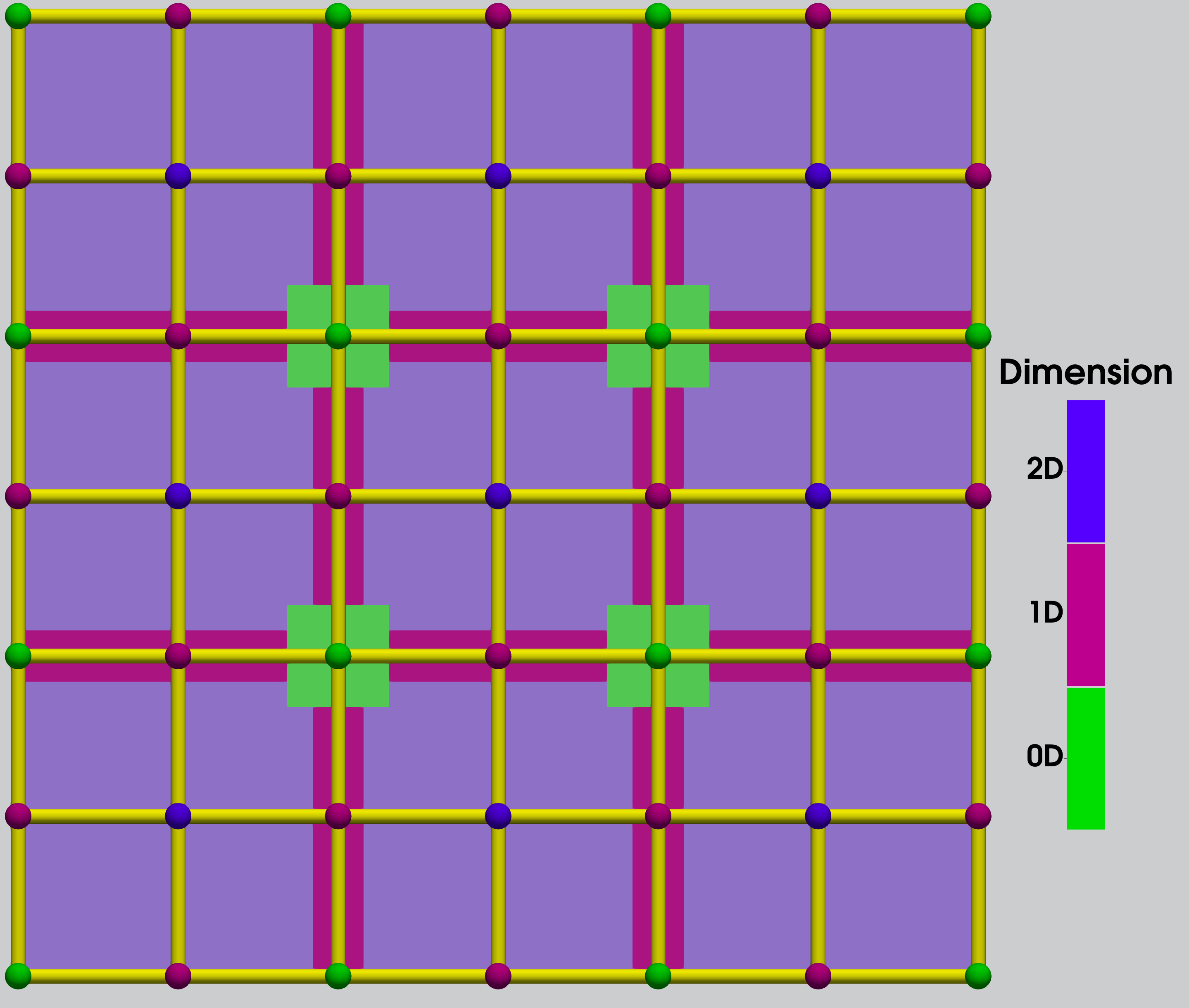
Two key assumptions are made in approximating the exact algorithm: spatial locality of the rules and well-separateness of cells of the same original dimensionality within the cell complex used to decompose the simulation space. Spatial locality, allows us to decompose the simulation space into smaller, well-separated geometric cells, or “geocells.” In the simulation algorithm, a “cell” refers to a computational spatial domain, not a biological cell. A geocell is a cell of an expanded cell complex (ECC), labeled by the dimension of the corresponding cell in the unexpanded complex. Lower-dimensional cells are expanded perpendicularly, so as to prevent rule instances from spanning multiple same-dimensional geocells. By setting these geocells wide enough (several times larger than the exponential “fall off distance” of local rule propensity functions), we can map rule instances using the to-be-discussed function to well-separated geocells. An example of an ECC can be found in figure 1.
The system state itself is a labeled graph with nodes labeled by vector-valued position parameters, also allowing additional parameters without spatial constraints. Our graph grammar rules are used to find matching graph patterns in the system graph and are made spatially local by their propensity functions, which define local neighborhoods of rule firings. Rule instantiations outside this neighborhood requires a fast enough e.g. exponential falloff with distance in the “with” rule propensity functions, and in turn they will have zero or near-zero propensity outside the neighborhood. Thus, interactions between distant objects are unlikely and can be ignored with minimal error e.g. in a chemical reaction, reactants that are very far away from one another do not interact.
The operator in is defined in the state space for all extended objects in the system. Let be the sum of the DGG rules mapped to operators. We can approximate the solution, , to the master equation by using operator splitting that imposes a domain decomposition by means of an expanded cell complex that corresponds to summing operators, , over pre-expansion dimensions , and cells of each dimension:
| (6a) | ||||
| (6b) | ||||
| (6c) | ||||
Sub-equation (6a) is a first-order operator splitting, by solution phases of fixed cell dimension, where means we multiply from right to left in order of highest dimension to lowest. It incurs an approximate error of . Sub-equation (6b) is an even stronger refinement of sub-equation (6a) because it uses the fact that the resulting cells of fixed dimension are all well-separated geometrically with enough margin (due to the expanded regionsRand and Walkington (2009) of dimension ) so that rule (reaction) instances , and commute to high accuracy if they are assigned to different cells of the same dimensionality, by some rule (reaction) instance allocation function . The commutators of equation (6b) can be calculated as derived in Mjolsness (2022), but they will inherit the product of two exponential falloffs with separation that we assumed for the rule propensities (c.f. Mjolsness (2022), equation 12 therein), which is an even faster exponential falloff. Hence the dynamics of different cells of the same original dimension and can be simulated in any order, or in parallel, at little cost in accuracy. The logic is expressed in Algorithm 1.
Algorithm 1 is the original version of the approximate algorithm and was run in serial for the model discussed in previous work Medwedeff and Mjolsness (2023). On the highest level, it specifies that must be used to map reaction instances to geocells and those have the potential to be processed in parallel or serial asynchronously. It fully encapsulates sub-equations (6b) and (6c). However, it leaves unspecified the details of how to keep the state of the rule matches in the simulated system consistent across geocells after a rule fires and a rewrite occurs.
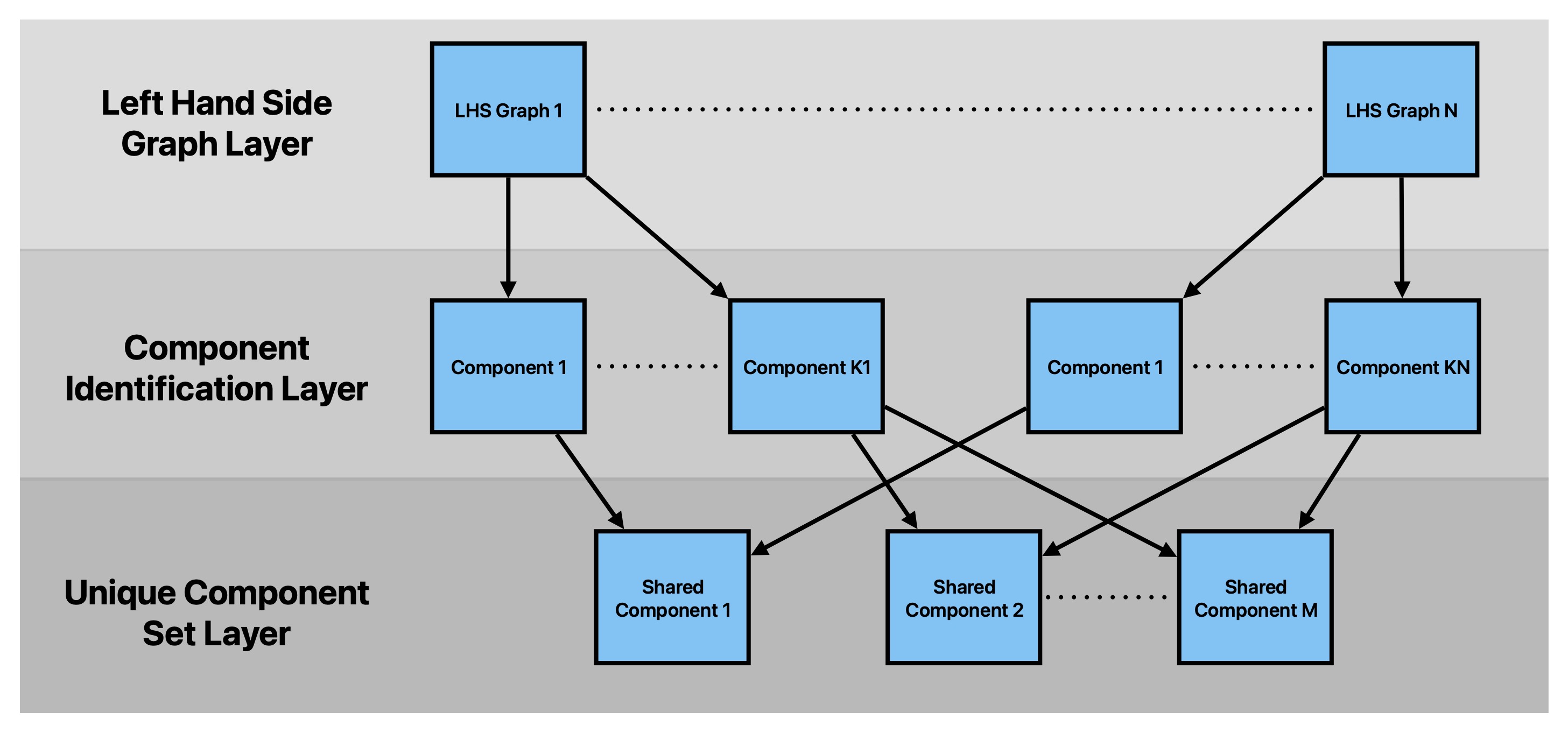
Algorithm 2, which is the algorithm used in DGGML, improves upon the original by adding in explicit requirements to efficiently keep the state of rule matches in the simulated system consistent across geocells after a rule fires and a rewrite occurs. To keep a consistent state of rule matches, we specify how rule matches are represented. The match data structure (visualized in figure 2), which is initialized at the beginning of Algorithm 2, is a data structure that stores all possible rule instances matching the grammar rules to all possible corresponding left-hand side (LHS) connected component instances. The match data structure is then the representation of all current rule instances and must be updated every time a rule fires and the system graph is rewritten. To make this work we take advantage of an incremental updating procedure (section II.5) within a geocell, which allows us not to have to recompute all new matches after distant events occur in the system.
Algorithm 2 also includes the point of synchronization and rule invalidation that comes after processing all expanded cells of a given dimension. After maps every rule to a cell of dimension , the exact algorithm running within is responsible for incrementally updating its state and keeping track of any rule invalidation that may share objects with rules belonging to neighboring cells of differing dimensions. Hence, the need for the synchronization point in Algorithm 2. Synchronizing for consistency is a consequence of the commutator approximation in equation (6b). When running in serial the synchronization point is still present and functions as a logical point in the algorithm for inserting any custom code for correcting and creating a consistent state of rule matches and potentially measuring any errors. Algorithm 2 also has the potential to be made parallel in a lock-free way thanks to the synchronization point, because it leaves the resolution of the global state until after the operation of all geocells of dimension , making it a substantial improvement over Algorithm 1.
Algorithm 2 also substantially improves upon Algorithm 1 by introducing the aforementioned match data structure with an incremental update process to ensure that distant rule firings do not require the matches to be recomputed and that full system matches are only ever recomputed when needed. The primary need for recomputation even after synchronization occurs because spatially embedded and spatially local graph grammar rules are composed of one or more distinct connected components. By virtue of solving rules, these components may move in or out of the propensity “fall-off” distance. While these connected components themselves can always be incrementally updated i.e. the set of connected component matches is fully online, the rule instances that comprise them can only be incrementally updated for a short period of time. As a result, they need to be recomputed periodically, making the match data structure semi-online.
In the absence of domain decomposition Algorithm 1 reduces to the exact algorithm, and Algorithm 2 reduces to a version of the exact algorithm but with the incremental update of the rule match data structure. A more complete mathematical treatment of the approximate algorithm using DGG commutators computed Mjolsness (2022) to bound operator splitting errors is a topic for future work. Algorithms 1 and 2 are specifically designed for spatially embedded graphs, but there are situations where they could be used in other non-spatial instances if we had a way to reasonably measure locality in the parameter space and that is another topic for future work. For DGGML Algorithm 2 is used, but we present Algorithm 1 as well to highlight the difference.
II.3 Yet Another Graph Libary (YAGL)
The DGG simulator relies on graphs as its core data structure but does not specify how to implement graph rewrites or represent graphs computationally. To address this, the Yet Another Graph Library (YAGL) was introducedMedwedeff and Mjolsness (2023) and further developed as a versatile, header-only library designed for compatibility with modern C++17 features. Unlike the monolithic Boost Graph LibrarySiek, Lee, and Lumsdaine (2002) (BGL), YAGL emphasizes flexibility and future extensibility without external dependencies. YAGL defines nodes, edges, and adjacency lists using static polymorphism and template meta-programming, with nodes stored in an unordered map for efficient lookup and edges in an unordered multi-map to support multiple edges between nodes. The adjacency list, realized as an unordered map, allows constant-time lookup of incoming and outgoing edges, facilitating dynamic graph operations.
YAGL includes operations such as adding/removing nodes and edges, identifying connected components, various graph searches, generating spanning trees, determining graph isomorphism, and solving the injective homomorphism problem for subgraph pattern recognition. For DGGML, which uses spatial graphs, YAGL implements a specialized spatial variadic templated variant node type, enabling dynamic type changes during graph rewrites while maintaining spatial data and user-defined values.
II.4 Phi Function
The process by which rules get mapped to a particular dimensional cell in Algorithm 2 hinges on the choice of the function in Equation (6c). This function plays a pivotal role in establishing a suitable mapping from reactions (rules) to geocells, ensuring that each reaction instance maps to exactly one geocell. This approach guarantees complete accountability for all rules. Because assigns a geometric cell to every match, serves to partition the set of matches. Various implementation choices exist for defining , each presenting distinct trade-offs. We will focus on two primary approaches to demonstrate how they work.
Assume that the following is a match of the left-hand side of a graph grammar rule, and the associated parameters and unique IDs are as follows:
Here, the match has a closed square type with integer ID and two open circle types with integer IDs and . Each of the graph grammar rules has an associated position vector . Let be a function that returns the unique cell id to which an object at position belongs and let the function be a function that returns the dimension of that cell. For example, assume that , , and . Also, assume , , and . Therefore, belongs to a cell of dimension , and the other nodes belong to cell of dimension . Also, keep in mind that the spatial-locality and well-separated constraints ensure that all matched objects in the rule will not belong to more than one cell of the same dimension. Thus, restricted to a given match, the function has an inverse .
The first approach we discuss uses the single-point anchored function, which involves selecting an “anchor node” from the left-hand side and determining the geocell containing its spatial coordinates. The selection of another node may be arbitrary or may be guided by a user-defined heuristic such as a root of a spanning tree. Using the section example, we could pick the root to be node . In this way, we have , which is a cell of dimension . Hence, a single-point anchored mapping function maps node to cell . This method boosts computational efficiency by necessitating only a single point for lookup. However, a trade-off arises wherein automorphisms of the same rule match may be assigned to different dimensions. When an invalidation occurs, each geocell containing the invalidate rule must be updated.
Alternatively, the minimum dimensions function can be defined to map the rule match to the minimum dimension of the geocells to which each node maps. Using the section example, it would be:
| (10) | ||||
| (11) |
which is a cell of dimension where exists by well-separatedness. This function can be further extended to consider all rules in which any node of the current rule participates. In either scenario, each instance of the function calculates the minimum dimension for any match and assigns the rule instance to the corresponding geocell. The well-separated property ensures that no node in the rule or its associated rules can be assigned to multiple geocells of identical dimensions. The minimum dimension ensures that all automorphisms are consistently assigned to the same dimension and cell because the function returns the same result, regardless of the ordering of the input. Computationally, the cost of using the minimum dimension means checking the spatial coordinates of each node on the left-hand side.
II.5 Incremental Update
The incremental update in Algorithm 2 is a critical improvement and results in a more efficient algorithmic realization of the DGG formalism. Once a rule is selected to fire and fires, the system’s state must be updated. The most straightforward approach would involve recomputing all matches in the systemMedwedeff and Mjolsness (2023), which is clearly resource intensive. The following discussion presents an alternative solution by incrementally updating the matches of the LHS of DGG rules found in the system.
Before proceeding, it is useful to clarify some terminology. In the context of DGGML, matches of the LHS graph for a rule are stored hierarchically. We store them in this way because the LHS graph of a grammar rule may be a graph with more than one connected component. This is what we mean by a multicomponent rule/graph. For example a collision-induced catastrophe rule from the PCMA grammar in Appendix LABEL:pcma_dgg:
Note: in rule LABEL:rule2:disc_growth and any other occurrence, is short for Heaviside, as in table 6.
A.2 Retraction Rules
Note: in rule LABEL:rule2:bnd_cic_std and any other occurrence, on a propositional True/False value as in table 6.
| (42) | |||
| (45) | |||
| (46) |
A.4 MT Collision Induced Catastrophe Rules
| (49) | |||
| (52) | |||
| (55) | |||
| (56) |
| (59) | |||
| (62) | |||
| (63) |
| (66) | |||
| (69) | |||
| (70) |
A.5 Crossover Rules
| (73) | |||
| (77) | |||
| (81) | |||
| (82) |
| (86) | |||
| (90) | |||
| (93) |
A.6 Zippering Rules
| (96) | |||
| (100) | |||
| (103) | |||
| (104) |
| (108) | |||
| (112) | |||
| (114) | |||
| (115) |
| (116) |
A.7 CLASP Rules
| (117) | |||
| (120) | |||
| (122) | |||
| (123) |
| (126) | |||
| (129) | |||
| (133) | |||
| (134) |
| (137) | |||
| (140) | |||
| (142) |
| (145) | |||
| (148) | |||
| (150) |
A.8 Destruction and Creation Rules
| (153) |
| (154) | ||||
| (157) | ||||
| (159) | ||||
| (163) | ||||
| (165) |
A.9 State Changes
| (166) |
A.10 Parameters and Symbols
| Rule Parameter | Description |
|---|---|
| a point in | |
| a unit vector in | |
| current length of the MT segment |
| Graph Symbol | Type Name |
|---|---|
| growing | |
| intermediate | |
| retraction | |
| zipper | |
| junction | |
| nucleator | |
| boundary |
| Model Parameter | Description | Value | Source |
|---|---|---|---|
| the maximal dividing length of a segment | 0.075 m | Estimated Burbank and Mitchison (2006); Elliott and Shaw (2017) | |
| growth rate | 0.0615 | Dixit and Cyr (2004); Allard, Wasteneys, and Cytrynbaum (2010) | |
| the minimal length of a segment | 0.0025 m | Estimated Burbank and Mitchison (2006); Elliott and Shaw (2017) | |
| retraction rate | 0.00883 | Dixit and Cyr (2004); Allard, Wasteneys, and Cytrynbaum (2010) | |
| CIC angle threshold | Estimated Dixit and Cyr (2004); Allard, Wasteneys, and Cytrynbaum (2010); Chakrabortty et al. (2018) | ||
| maximal reaction radius | 0.1 m | Estimated Burbank and Mitchison (2006); Elliott and Shaw (2017) | |
| critical zippering angle threshold | Dixit and Cyr (2004); Ambrose and Wasteneys (2008) | ||
| MT separation distance | 0.025 m | Chan et al. (1999) | |
| crossover angle threshold | Estimated Dixit and Cyr (2004); Allard, Wasteneys, and Cytrynbaum (2010); Chakrabortty et al. (2018) | ||
| CLASP entry angle threshold | Estimated Vineyard et al. (2013) | ||
| CLASP exit angle threshold | Estimated Vineyard et al. (2013) | ||
| MT collision distance | 0.025 m | Estimated Chakrabortty et al. (2018); Elliott and Shaw (2017) | |
| Minimum MT segment initialization length | 0.005 m | Estimated Elliott and Shaw (2017) | |
| Minimum MT segment initialization length | 0.01 m | Estimated Elliott and Shaw (2017) |
| Model Parameter | Description | Propensity Rate | Source |
|---|---|---|---|
| growth rate factor | 100.0 | Estimated | |
| retraction rate factor | 10.0 | Estimated | |
| boundary CIC standard rate factor | 40,000 | Estimated | |
| boundary CIC for CLASP rate factor | 40,000 | Estimated | |
| intermediate CIC rate factor | 12,000 | Estimated Dixit and Cyr (2004) | |
| growing end CIC rate factor | 12,000 | Estimated Dixit and Cyr (2004) | |
| retracting end CIC rate factor | 12,000 | Estimated Dixit and Cyr (2004) | |
| zippering entrainment rate factor | 4,000 | Estimated Dixit and Cyr (2004) | |
| zippering guard rate factor | 12,000 | Estimated Dixit and Cyr (2004) | |
| crossover rate factor | 200 | Estimated Dixit and Cyr (2004) | |
| uncrossover rate factor | 0.01 | Estimated | |
| clasp entry rate factor | 0.001 | Estimated Vineyard et al. (2013); Sambade et al. (2012) | |
| clasp exit rate factor | 40,000 | Estimated Vineyard et al. (2013); Sambade et al. (2012) | |
| clasp catastrophe rate factor | 1,000 | Estimated | |
| clasp detachment rate factor | 0.016 | Estimated | |
| destruction rate factor | 0.0026 | Estimated | |
| creation rate factor | 0.0026 | Estimated Allard, Wasteneys, and Cytrynbaum (2010) | |
| retraction to growth conversion rate | 0.016 | Estimated Wightman and Turner (2007) | |
| growth to retraction conversion rate | 0.016 | Estimated Wightman and Turner (2007) |
| Function | Description |
|---|---|
|
Minimum distance
from to the line through and |
|
|
Given a point
in the direction find the angle made with |
|
| Heaviside function | |
| rotation function | |
| indication function | |
| Line intersection |
References
- Diestel (2017) R. Diestel, Graph Theory, 5th ed. (Springer, 2017) Chap. 1, pp. 1–31.
- Mjolsness (2013) E. Mjolsness, “Time-ordered product expansions for computational stochastic system biology,” Physical Biology 10, 035009 (2013).
- Mjolsness (2022) E. Mjolsness, “Explicit calculation of structural commutation relations for stochastic and dynamical graph grammar rule operators in biological morphodynamics,” Frontiers in Systems Biology 2 (2022), 10.3389/fsysb.2022.898858.
- Rozenberg (1997) G. Rozenberg, Handbook of Graph Grammars and Computing by Graph Transformation (WORLD SCIENTIFIC, 1997).
- Mjolsness (2019) E. Mjolsness, “Prospects for declarative mathematical modeling of complex biological systems,” Bulletin of Mathematical Biology 81, 3385–3420 (2019).
- Gillespie (1977) D. T. Gillespie, “Exact stochastic simulation of coupled chemical reactions,” The Journal of Physical Chemistry 81, 2340–2361 (1977).
- Young and Elcock (1966) W. M. Young and E. W. Elcock, “Monte carlo studies of vacancy migration in binary ordered alloys: I,” Proceedings of the Physical Society 89, 735–746 (1966).
- Medwedeff and Mjolsness (2023) E. Medwedeff and E. Mjolsness, “Approximate simulation of cortical microtubule models using dynamical graph grammars,” Physical Biology 20, 055002 (2023).
- Metropolis et al. (1953) N. Metropolis, A. W. Rosenbluth, M. N. Rosenbluth, A. H. Teller, and E. Teller, “Equation of State Calculations by Fast Computing Machines,” The Journal of Chemical Physics 21, 1087–1092 (1953).
- Lecca, Laurenzi, and Jordan (2013a) P. Lecca, I. Laurenzi, and F. Jordan, “4 - modelling in systems biology,” in Deterministic Versus Stochastic Modelling in Biochemistry and Systems Biology, Woodhead Publishing Series in Biomedicine, edited by P. Lecca, I. Laurenzi, and F. Jordan (Woodhead Publishing, 2013) pp. 117–180.
- Lecca, Laurenzi, and Jordan (2013b) P. Lecca, I. Laurenzi, and F. Jordan, “1 - deterministic chemical kinetics,” in Deterministic Versus Stochastic Modelling in Biochemistry and Systems Biology, Woodhead Publishing Series in Biomedicine, edited by P. Lecca, I. Laurenzi, and F. Jordan (Woodhead Publishing, 2013) pp. 1–34.
- Bortz, Kalos, and Lebowitz (1975) A. Bortz, M. Kalos, and J. Lebowitz, “A new algorithm for monte carlo simulation of ising spin systems,” Journal of Computational Physics 17, 10–18 (1975).
- Gillespie (1992) D. T. Gillespie, “A rigorous derivation of the chemical master equation,” Physica A: Statistical Mechanics and its Applications 188, 404–425 (1992).
- Gillespie (2001) D. T. Gillespie, “Approximate accelerated stochastic simulation of chemically reacting systems,” The Journal of Chemical Physics 115, 1716–1733 (2001).
- Cao, Gillespie, and Petzold (2006) Y. Cao, D. T. Gillespie, and L. R. Petzold, “Efficient step size selection for the tau-leaping simulation method,” The Journal of Chemical Physics 124, 044109 (2006).
- Auger, Chatelain, and Koumoutsakos (2006) A. Auger, P. Chatelain, and P. Koumoutsakos, “R-leaping: Accelerating the stochastic simulation algorithm by reaction leaps,” The Journal of Chemical Physics 125, 084103 (2006).
- Mjolsness et al. (2009) E. Mjolsness, D. Orendorff, P. Chatelain, and P. Koumoutsakos, “An exact accelerated stochastic simulation algorithm,” The Journal of Chemical Physics 130, 144110 (2009).
- Orendorff and Mjolsness (2012) D. Orendorff and E. Mjolsness, “A hierarchical exact accelerated stochastic simulation algorithm,” The Journal of Chemical Physics 137, 214104 (2012).
- Lipková et al. (2019) J. Lipková, G. Arampatzis, P. Chatelain, B. Menze, and P. Koumoutsakos, “S-leaping: An adaptive, accelerated stochastic simulation algorithm, bridging -leaping and r-leaping,” Bulletin of Mathematical Biology 81, 3074–3096 (2019).
- Mjolsness and Yosiphon (2007) E. Mjolsness and G. Yosiphon, “Stochastic process semantics for dynamical grammars,” Annals of Mathematics and Artificial Intelligence 47, 329–395 (2007).
- Mjolsness (2010) E. Mjolsness, “Towards measurable types for dynamical process modeling languages,” Electronic notes in theoretical computer science 265, 123–144 (2010).
- Yosiphon and Mjolsness (2009) G. Yosiphon and E. Mjolsness, Learning and Inference in Computational Systems Biology (MIT Press, 2009) pp. 297–314.
- Yosiphon (2009) G. Yosiphon, Stochastic Parameterized Grammars : Formalization, Inference and Modeling Applications, Ph.D. thesis, UC Irvine (2009).
- Wolfram Research, Inc. (2021) Wolfram Research, Inc., “Mathematica,” (2021).
- Dechter (1997) R. Dechter, “Bucket elimination: a unifying framework for processing hard and soft constraints,” Constraints 2, 51–55 (1997).
- Dechter (2003) R. Dechter, Constraint Processing, The Morgan Kaufmann Series in Artificial Intelligence (Morgan Kaufmann, San Francisco, 2003).
- Giavitto and Michel (2001) J.-L. Giavitto and O. Michel, “Mgs: A rule-based programming language for complex objects and collections,” Electronic Notes in Theoretical Computer Science 59, 286–304 (2001), rULE 2001, Second International Workshop on Rule-Based Programming (Satellite Event of PLI 2001).
- Stiles, Bartol et al. (2001) J. R. Stiles, T. M. Bartol, et al., “Monte carlo methods for simulating realistic synaptic microphysiology using mcell,” Computational neuroscience: Realistic modeling for experimentalists , 87–127 (2001).
- Shapiro and Mjolsness (2015) B. E. Shapiro and E. Mjolsness, “Pycellerator: an arrow-based reaction-like modelling language for biological simulations,” Bioinformatics 32, 629–631 (2015).
- Blinov et al. (2004) M. L. Blinov, J. R. Faeder, B. Goldstein, and W. S. Hlavacek, “BioNetGen: software for rule-based modeling of signal transduction based on the interactions of molecular domains,” Bioinformatics 20, 3289–3291 (2004).
- Harris et al. (2016) L. A. Harris, J. S. Hogg, J.-J. Tapia, J. A. P. Sekar, S. Gupta, I. Korsunsky, A. Arora, D. Barua, R. P. Sheehan, and J. R. Faeder, “BioNetGen 2.2: advances in rule-based modeling,” Bioinformatics 32, 3366–3368 (2016).
- Danos and Laneve (2004) V. Danos and C. Laneve, “Formal molecular biology,” Theoretical Computer Science 325, 69–110 (2004), computational Systems Biology.
- Spicher and Michel (2007) A. Spicher and O. Michel, “Declarative modeling of a neurulation-like process,” Biosystems 87, 281–288 (2007), papers presented at the Sixth International Workshop on Information Processing in Cells and Tissues, York, UK, 2005.
- Lane (2015) B. Lane, Cell Complexes: The Structure of Space and the Mathematics of Modularity, Ph.D. thesis, University of Calgary Computer Science Department (2015).
- Shapiro et al. (2003) B. E. Shapiro, A. Levchenko, E. M. Meyerowitz, B. J. Wold, and E. Mjolsness, “Cellerator: extending a computer algebra system to include biochemical arrows for signal transduction simulations,” Bioinform. 19, 677–678 (2003).
- Deeds et al. (2012) E. J. Deeds, J. Krivine, J. Feret, V. Danos, and W. Fontana, “Combinatorial complexity and compositional drift in protein interaction networks,” PLOS ONE 7, 1–14 (2012).
- Rand and Walkington (2009) A. Rand and N. Walkington, “Collars and intestines: Practical conforming Delaunay refinement,” in Proceedings of the 18th International Meshing Roundtable, edited by B. W. Clark (Springer, Berlin, 2009) pp. 481–497.
- Siek, Lee, and Lumsdaine (2002) J. Siek, L.-Q. Lee, and A. Lumsdaine, “The boost graph library: User guide and reference manual,” (2002).
- Allen and Tildesley (2017) M. P. Allen and D. J. Tildesley, Computer Simulation of Liquids (Oxford University Press, 2017).
- Löwe (1993) M. Löwe, “Algebraic approach to single-pushout graph transformation,” Theoretical Computer Science 109, 181–224 (1993).
- Ehrig, Pfender, and Schneider (1973) H. Ehrig, M. Pfender, and H. J. Schneider, “Graph-grammars: An algebraic approach,” in 14th Annual Symposium on Switching and Automata Theory (swat 1973) (1973) pp. 167–180.
- Valiente (2021) G. Valiente, “Graph isomorphism,” in Algorithms on Trees and Graphs: With Python Code (Springer International Publishing, Cham, 2021) pp. 255–285.
- Coen and Cosgrove (2023) E. Coen and D. J. Cosgrove, “The mechanics of plant morphogenesis,” Science 379, eade8055 (2023).
- Shaw (2013) S. L. Shaw, “Reorganization of the plant cortical microtubule array,” Current Opinion in Plant Biology 16, 693–697 (2013), cell biology.
- Elliott and Shaw (2017) A. Elliott and S. L. Shaw, “Update: Plant Cortical Microtubule Arrays,” Plant Physiology 176, 94–105 (2017).
- Abrash and Bergmann (2009) E. B. Abrash and D. C. Bergmann, “Asymmetric cell divisions: A view from plant development,” Developmental Cell 16, 783–796 (2009).
- Allard, Wasteneys, and Cytrynbaum (2010) J. F. Allard, G. O. Wasteneys, and E. N. Cytrynbaum, “Mechanisms of self-organization of cortical microtubules in plants revealed by computational simulations,” Molecular Biology of the Cell 21, 278–286 (2010), pMID: 19910489.
- Tindemans et al. (2014) S. Tindemans, E. Deinum, J. Lindeboom, and B. Mulder, “Efficient event-driven simulations shed new light on microtubule organization in the plant cortical array,” Frontiers in Physics 2 (2014), 10.3389/fphy.2014.00019.
- Eren, Dixit, and Gautam (2010) E. C. Eren, R. Dixit, and N. Gautam, “A three-dimensional computer simulation model reveals the mechanisms for self-organization of plant cortical microtubules into oblique arrays,” Molecular Biology of the Cell 21, 2674–2684 (2010), pMID: 20519434.
- Thoms et al. (2018) D. Thoms, L. Vineyard, A. Elliott, and S. L. Shaw, “CLASP Facilitates Transitions between Cortical Microtubule Array Patterns,” Plant Physiology 178, 1551–1567 (2018).
- Ambrose et al. (2011) C. Ambrose, J. F. Allard, E. N. Cytrynbaum, and G. O. Wasteneys, “A clasp-modulated cell edge barrier mechanism drives cell-wide cortical microtubule organization in arabidopsis,” Nature Communications 2, 430 (2011).
- Tindemans, Hawkins, and Mulder (2010) S. Tindemans, R. Hawkins, and B. Mulder, “Survival of the aligned: Ordering of the plant cortical microtubule array,” Physical review letters 104, 058103 (2010).
- Schneider et al. (2021) R. Schneider, K. v. Klooster, K. L. Picard, J. van der Gucht, T. Demura, M. Janson, A. Sampathkumar, E. E. Deinum, T. Ketelaar, and S. Persson, “Long-term single-cell imaging and simulations of microtubules reveal principles behind wall patterning during proto-xylem development,” Nature Communications 12, 669 (2021).
- Vineyard et al. (2013) L. Vineyard, A. Elliott, S. Dhingra, J. R. Lucas, and S. L. Shaw, “Progressive Transverse Microtubule Array Organization in Hormone-Induced Arabidopsis Hypocotyl Cells,” The Plant Cell 25, 662–676 (2013).
- Sambade et al. (2012) A. Sambade, A. Pratap, H. Buschmann, R. J. Morris, and C. Lloyd, “The Influence of Light on Microtubule Dynamics and Alignment in the Arabidopsis Hypocotyl,” The Plant Cell 24, 192–201 (2012).
- Chan et al. (1999) J. Chan, C. G. Jensen, L. C. Jensen, M. Bush, and C. W. Lloyd, “The 65-kda carrot microtubule-associated protein forms regularly arranged filamentous cross-bridges between microtubules,” Proceedings of the National Academy of Sciences 96, 14931–14936 (1999).
- Murata et al. (2005) T. Murata, S. Sonobe, T. I. Baskin, S. Hyodo, S. Hasezawa, T. Nagata, T. Horio, and M. Hasebe, “Microtubule-dependent microtubule nucleation based on recruitment of -tubulin in higher plants,” Nature Cell Biology 7, 961–968 (2005).
- Nakamura and Hashimoto (2009) M. Nakamura and T. Hashimoto, “A mutation in the Arabidopsis -tubulin-containing complex causes helical growth and abnormal microtubule branching,” Journal of Cell Science 122, 2208–2217 (2009).
- Wightman et al. (2013) R. Wightman, G. Chomicki, M. Kumar, P. Carr, and S. Turner, “Spiral2 determines plant microtubule organization by modulating microtubule severing,” Current Biology 23, 1902–1907 (2013).
- Himmelspach, Williamson, and Wasteneys (2003) R. Himmelspach, R. E. Williamson, and G. O. Wasteneys, “Cellulose microfibril alignment recovers from dcb-induced disruption despite microtubule disorganization,” The Plant Journal 36, 565–575 (2003).
- Baulin, Marques, and Thalmann (2007) V. A. Baulin, C. M. Marques, and F. Thalmann, “Collision induced spatial organization of microtubules,” Biophysical Chemistry 128, 231–244 (2007).
- Deinum et al. (2017) E. E. Deinum, S. H. Tindemans, J. J. Lindeboom, and B. M. Mulder, “How selective severing by katanin promotes order in the plant cortical microtubule array,” Proceedings of the National Academy of Sciences 114, 6942–6947 (2017).
- Pampaloni et al. (2006) F. Pampaloni, G. Lattanzi, A. Jonáš, T. Surrey, E. Frey, and E.-L. Florin, “Thermal fluctuations of grafted microtubules provide evidence of a length-dependent persistence length,” Proceedings of the National Academy of Sciences 103, 10248–10253 (2006).
- de Moura et al. (2015) L. de Moura, S. Kong, J. Avigad, F. van Doorn, and J. von Raumer, “The lean theorem prover (system description),” in Automated Deduction - CADE-25, edited by A. P. Felty and A. Middeldorp (Springer International Publishing, Cham, 2015) pp. 378–388.
- Ernst et al. (2018) O. K. Ernst, T. Bartol, T. Sejnowski, and E. Mjolsness, “Learning dynamic boltzmann distributions as reduced models of spatial chemical kinetics,” The Journal of Chemical Physics 149, 034107 (2018).
- Scott and Mjolsness (2019) C. B. Scott and E. Mjolsness, “Multilevel artificial neural network training for spatially correlated learning,” SIAM Journal on Scientific Computing 41, S297–S320 (2019).
- Eric Medwedeff (2024) E. M. Eric Medwedeff, “The dynamical graph grammar modeling library,” https://github.com/emedwede/DGGML (2024).
- Medwedeff (2023) E. Medwedeff, “Yet another graph library,” https://github.com/emedwede/YAGL (2023).
- Burbank and Mitchison (2006) K. S. Burbank and T. J. Mitchison, “Microtubule dynamic instability,” Current Biology 16, R516–R517 (2006).
- Dixit and Cyr (2004) R. Dixit and R. Cyr, “Encounters between Dynamic Cortical Microtubules Promote Ordering of the Cortical Array through Angle-Dependent Modifications of Microtubule Behavior,” The Plant Cell 16, 3274–3284 (2004).
- Chakrabortty et al. (2018) B. Chakrabortty, V. Willemsen, T. de Zeeuw, C.-Y. Liao, D. Weijers, B. Mulder, and B. Scheres, “A plausible microtubule-based mechanism for cell division orientation in plant embryogenesis,” Current Biology 28, 3031–3043.e2 (2018).
- Ambrose and Wasteneys (2008) J. C. Ambrose and G. O. Wasteneys, “Clasp modulates microtubule-cortex interaction during self-organization of acentrosomal microtubules,” Molecular biology of the cell 19, 4730–4737 (2008).
- Wightman and Turner (2007) R. Wightman and S. R. Turner, “Severing at sites of microtubule crossover contributes to microtubule alignment in cortical arrays,” The Plant Journal 52, 742–751 (2007).