*[inlinelist,1]label=(),
Adversarial Attacks are a Surprisingly Strong Baseline for Poisoning Few-Shot Meta-Learners
Abstract
This paper examines the robustness of deployed few-shot meta-learning systems when they are fed an imperceptibly perturbed few-shot dataset. We attack amortized meta-learners, which allows us to craft colluding sets of inputs that are tailored to fool the system’s learning algorithm when used as training data. Jointly crafted adversarial inputs might be expected to synergistically manipulate a classifier, allowing for very strong data-poisoning attacks that would be hard to detect. We show that in a white box setting, these attacks are very successful and can cause the target model’s predictions to become worse than chance. However, in opposition to the well-known transferability of adversarial examples in general, the colluding sets do not transfer well to different classifiers. We explore two hypotheses to explain this: “overfitting” by the attack, and mismatch between the model on which the attack is generated and that to which the attack is transferred. Regardless of the mitigation strategies suggested by these hypotheses, the colluding inputs transfer no better than adversarial inputs that are generated independently in the usual way.
1 Introduction
Standard deep learning approaches suffer from poor sample efficiency (Krizhevsky et al., 2012) which is problematic in tasks where data collection is difficult or expensive. Few-shot learners have been developed to address this shortcoming by supporting rapid adaptation to a new task using only a few labeled examples (Finn et al., 2017; Snell et al., 2017). This success has made few-shot learners more attractive for increasingly sensitive applications where the repercussions of confidently-wrong predictions are severe, such as clinical risk assessment (Sheryl Zhang et al., 2019), glaucoma diagnosis (Kim et al., 2017) and diseases identification in skin lesions (Mahajan et al., 2020).
As few-shot learners gain popularity, it is essential to understand how robust they are and how they may be exploited. It is well known that standard classifiers are vulnerable to adversarial inputs which have been purposefully and imperceptibly modified to cause incorrect predictions (Biggio and Roli, 2017). Such examples may be presented to a model either at test time, called evasion attacks (Biggio et al., 2017) or adversarial examples (Szegedy et al., 2014), or at training time, which is referred to as poisoning (Newsome et al., 2006; Rubinstein et al., 2009). The concepts of evasion and poisoning can be re-stated in terms of few-shot learners. At meta-test time, a few-shot learner is presented with an unseen task containing a few labeled examples, the support set, and a number of unlabeled examples to classify, called the query set. We can perpetrate a “standard” adversarial attack by perturbing an image in the query set or perform a poisoning attack by perturbing images in the support set.
In this paper, we propose a poisoning attack against amortized meta-learners that jointly optimizes attack images through the meta-learner’s adaptation mechanism. We produce a colluding set of adversarial images that is explicitly tailored to fool the learning algorithm. We consider as a baseline the insertion of standard adversarial attack images into the support set. We expect our attack to perform better than this baseline, since standard adversarial attacks are optimised individually to cause misclassification by a fixed classifier (rather than being curated as a set to fool the adaptation mechanism itself). We may also expect the new attack to transfer to other learners, especially considering the well-known transferability of adversarial examples in literature Goodfellow et al. (2014); Papernot et al. (2016a); Szegedy et al. (2014). Our contributions are as follows:
-
1.
We define a poisoning attack on few-shot classifiers, referred to as adversarial support poisoning (ASP) or simply as support attacks. This applies coordinated adversarial perturbations to produce a colluding set of inputs, generated by jointly backpropagating through the meta-learner’s adaptation process to minimize model accuracy over a set of query points. To the best of the authors’ knowledge, ours is the first work to perpetrate poisoning attacks on trained few-shot classifiers.
-
2.
In a white box setting ASP is a very strong attack, far more effective than the baseline.
-
3.
Surprisingly, we show that ASP attacks do not transfer significantly better than the swap attack baseline, which inserts adversarial examples generated “in the usual way” into the support set.
-
4.
We observe that transferability of support attacks are highly dependent on the feature extractor used by the meta-learner. Although we propose various mitigation strategies to improve the transferability of support set attacks, we do not succeed at significantly improving over the efficacy of a swap attack, which is simpler and cheaper.
The last two findings are unexpected: we expect the ASP attack to be significantly stronger than the swap attack baseline because it is tailored to fool the learner’s adaptation process, is optimized over a set of query points and is able to collude within the adversarial set.
2 Background
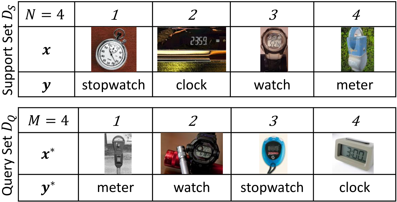
We focus on image classification, denoting input images by where is the image width, the image height, the number of image channels and image labels where is the number of image classes. We use bold and to denote sets of images and labels. We consider the few-shot image classification scenario using a meta-learning approach. Rather than a single, large dataset , we assume access to a dataset comprising a large number of training tasks , drawn i.i.d. from a distribution . An example task is shown in Fig.˜4. The data for a task consists of a support set comprising elements, with the inputs and labels observed, and a query set with elements for which we wish to make predictions. We may use the shorthand and . The meta-learner takes as input the support set and produces task-specific classifier parameters which are used to adapt the classifier to the current task. The classifier can now make task-specific predictions for any test input . Here the inputs are observed and the labels are only observed during meta-training (i.e. training of the meta-learning algorithm). Note that the query set examples are drawn from the same set of labels as the examples in the support set. The majority of modern meta-learning methods employ episodic training (Vinyals et al., 2016), as detailed in A.1. At meta-test time, the classifier is required to make predictions for query set inputs of unseen tasks, which will often include classes that have not been seen during meta-training, and will contain only a few observations.
The canonical example for modern gradient-based few-shot learning systems is MAML (Finn et al., 2017). Another widely used class of meta-learners are amortized-inference or black box based approaches e.g, Versa (Gordon et al., 2019) and CNAPs (Requeima et al., 2019a). In these methods, the task-specific parameters are generated by one or more hyper-networks, (Ha et al., 2016). Prototypical Networks (ProtoNets) (Snell et al., 2017) is a special case of this which is based on metric learning and employs a nearest neighbor classifier. We focuses on Simple CNAPs Bateni et al. (2020) – which improves on the performance of CNAPs – and uses a ProtoNets classifier head with an adaptive feature extractor like that of CNAPs; but we have also considered attacks against MAML, ProtoNets, and CNAPs with similar outcomes.
3 Attacking Few-Shot Learners
We summarize the threat model in terms of the adversary’s goal, capabilities and knowledge. In this work, we develop poisoning attacks that degrade the model availability (i.e. affect prediction results indiscriminately such that it is useless) (Jagielski et al., 2018). We allow the attacker to manipulate some fraction of the support set and further constrain pattern modifications to be imperceptible (i.e. within some of the original image, measured using the norm). When considering transfer attacks, we call the model used generate the attack the surrogate and the model to which we transfer the attack the target. We presume access to the surrogate model’s gradients and internal state. We don’t assume any access to the target model’s internal state, though some of the experiments do access a limited number of the target’s predictions. We also assume access to enough data to form a query set.
Consider a target model that has been trained and deployed as a service. As described in Section 1, a malicious party could perpetrate two kinds of attacks: a “standard” adversarial attack (hereafter referred to as a query attack) by perturbing elements in the query set of a task; or perform a poisoning attack by perturbing elements in the support set. We expand on these below:
Query Attack
Given a meta-learner that has already adapted to a specific task, the attacker perturbs a single test input in such a way that it will be misclassified. This corresponds to solving . Refer to Section˜A.6 for details. These attacks are essentially evasion attacks as considered in Biggio et al. (2017) and many algorithms can be used to generate adversarial examples (Madry et al., 2017; Carlini and Wagner, 2017; Chen et al., 2017). Query attacks have been perpetrated successfully against few-shot learners (Goldblum et al., 2019; Yin et al., 2018).
Adversarial Support Poisoning (ASP)
The attacker perturbs the dataset that the target meta-learner will learn from so as to influence all future test predictions. The attacker thus computes a perturbed support set whose inputs are jointly optimized to fool the system on a specific query set, which we call the seed query set, with the goal of generalizing to unseen query sets. This corresponds to solving such that , where denotes the seed query set and is the maximum size of the perturbation. Refer to Algorithm˜1 for details. Our attack is a poisoning attack, since the attacker is manipulating data that the model will use to do inference. However, it is important to note the the attack is perpetrated at meta-test time, after the meta-learner has already been meta-trained. Unlike a query attack, which is generated by backpropagating through the adapted learner with respect to a single point, our attack backpropagates jointly through the adaptation process with respect to the loss on the entire query set and should thus be a much stronger poisoning attack than say, inserting a query point into the support set. Without loss of generality, we use Projected Gradient Descent (PGD) (Madry et al., 2017) to generate perturbed support sets because it is effective, simple to implement, and easily extensible to sets of inputs.
4 Experiments
The experiments presented in the main body of the paper are carried out on Simple CNAPs (Bateni et al., 2020) using the challenging Meta-Dataset benchmark (refer to Section˜A.2 and for details on the meta-data training protocols and Meta-Dataset). The Simple CNAPs model uses a ProtoNets head in conjunction with an adaptive feature extractor. The ProtoNets head uses Euclidean distance and the feature extractor is a Resnet18 endowed with Feature-wise Linear Modulation (FiLM) layers (Perez et al., 2018), which scales and shifts a feature map by . In the meta-learning setting, FiLM parameters are generated by an adaptation network as part of , the learner’s adaptation to a new task, and allows the feature extractor to adapt flexibly to each new task with relatively few additional parameters (Requeima et al., 2019a). In Meta-Dataset, task support sets may be large — up to 500 images across all classes. In a realistic scenario, an attacker would not likely be able to perturb all the images in such a large support set, so we only perturb a specified fraction of the support set in each experiment. Each task is composed of a support set, a seed query set and up to 50 unseen query sets used for attack evaluation (some Meta-Dataset benchmarks do not have sufficiently many patterns available to form 50 query sets and thus were excluded from the experiments). The unseen query sets are all disjoint from the seed query set to avoid information leakage. For each task, we generate an adversarial support set using the original support set and corresponding seed query set. The adversarial support set is then evaluated on the task’s unseen query sets. We refer to the average classification accuracy on the seed query sets as the ASP Specific attack accuracy, and when evaluating the attack on unseen query sets we refer to it as the ASP General attack accuracy. An important baseline is the swap attack, which is generated by using the task’s support set and query set to produce a query attack, then “swap” the role of the adversarial query set by using it as a support set. Like our ASP attack, the swap attack is evaluated on unseen query sets. Note that the swap attack is far less expensive to compute than the ASP attack, since it only requires backpropagation through the adapted learner and not through the entire meta-learning process.
4.1 White Box Attack
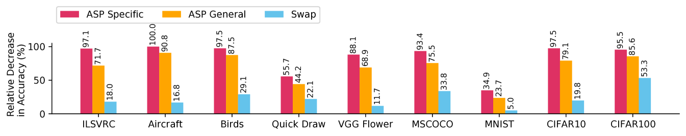
We first consider the simplest scenario, a white box attack in which the surrogate and target model are the same. Fig.˜1 shows the relative decrease in accuracy of Simple CNAPs on Meta-Dataset. In general, the clean accuracy of the surrogate and target models may be quite different and so we normalise the effect an attack has by computing the percentage relative decrease in classification accuracy as follows: where is the clean classification accuracy before the attack, and is the classification accuracy after the attack. Unnormalised results are in A.5. Although it is expected for ASP Specific to be very effective, the ASP attack remains highly effective even on unseen query sets (see ASP General), easily out-performing the Swap baseline, in spite of the fact that only of the support set shots are poisoned. At least in the white box setting, ASP is very strong attack.
4.2 Attack Transfer
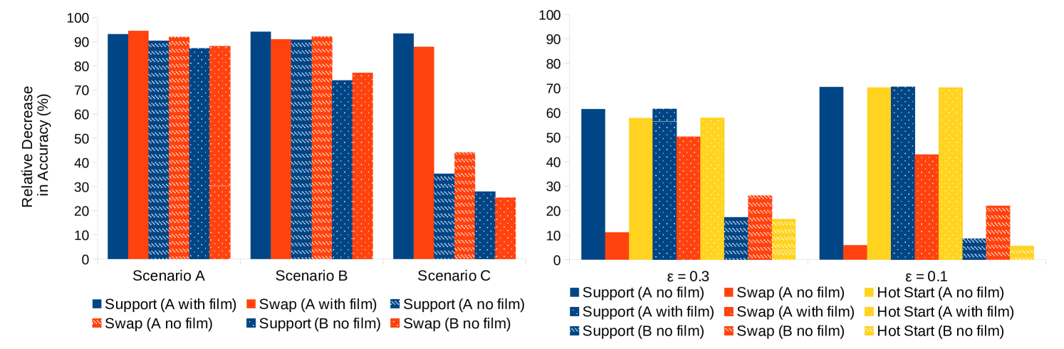
We now turn our attention to the more difficult scenario, in which the target and surrogate models are different. We fix our surrogate model as Simple CNAPs with a particular Resnet18 feature extractor (hereafter referred to Resnet18 A). We consider a Simple CNAPs model with a slightly different feature extractor: Resnet18 B, which was trained on the same data with similar training conditions, but with no FiLM parameters. We also consider turning the FiLM parameters for Resnet18 A on and off. Although this seems a rather trivial extension, the results shown in Fig.˜2 indicate that the ASP attack no longer outperforms the Swap baseline by a statistically significant margin. Fig.˜2 considers three scenarios in increasing order of difficulty. For Scenario A, the perturbation size is very large () and the entire support set has been adversarially perturbed. At this scale, tampering could be clearly inferred by inspection and it is unlikely that an adversary would have control over the entire support set, so this is the weakest scenario. In this setting, we see good transfer between the surrogate model, Resnet18 A with FiLM, and the target models (Resnet18 A without FiLM and Resnet18 B without FiLM). Scenario B reduces the perturbation size to be mostly imperceptible (), but still perturbs the entire support set. Here, we start to see a reduction in attack effectiveness when transferring to Resnset18 B. In Scenario C, we use and also reduce the proportion of poisoned samples in the support set to . Here we see significant reduction in transfer, even to Resnet18 A without FiLM. We also note that unlike the white box attack, we do not perform significantly better than the Swap attack, and possibly perform a little worse.
We know from literature that adversarial attacks transfer well and should thus be fairly robust to the kind of feature extractor being used. Since we’re only changing the feature extractor and keeping the type of learner the same, we expect the support attacks, which are tailored to fool the learning mechanism, to have a benefit over the swap attack. However, this is not borne out in experiments. We consider two avenues of explanation that account for the poor transfer between feature extractors: mismatch between the target and surrogate models, and “overfitting” of the attack to the support set and/or surrogate model. We consider a number of mitigation strategies intended to address these two problems below:
Decision Boundary Alignment
Since the target and surrogate models have different feature extractors, it may be that their embedding spaces and consequently also their decision boundaries are very different. We can try to “re-align” the surrogate model’s decision boundaries by training it to produce the same predictions as the target model, an approach which has been used in literature when perpetrating transfer attacks (Papernot et al., 2016b). In a meta-learning setting, this corresponds to relabeling the support set presented to the surrogate model based on the target model’s predictions. The labels of the support set when presented to the surrogate model will thus not be the true labels, but rather the labels assigned to the support images by the target model. The relabeled support set is also used to generate the swap attack so that the comparison is fair.
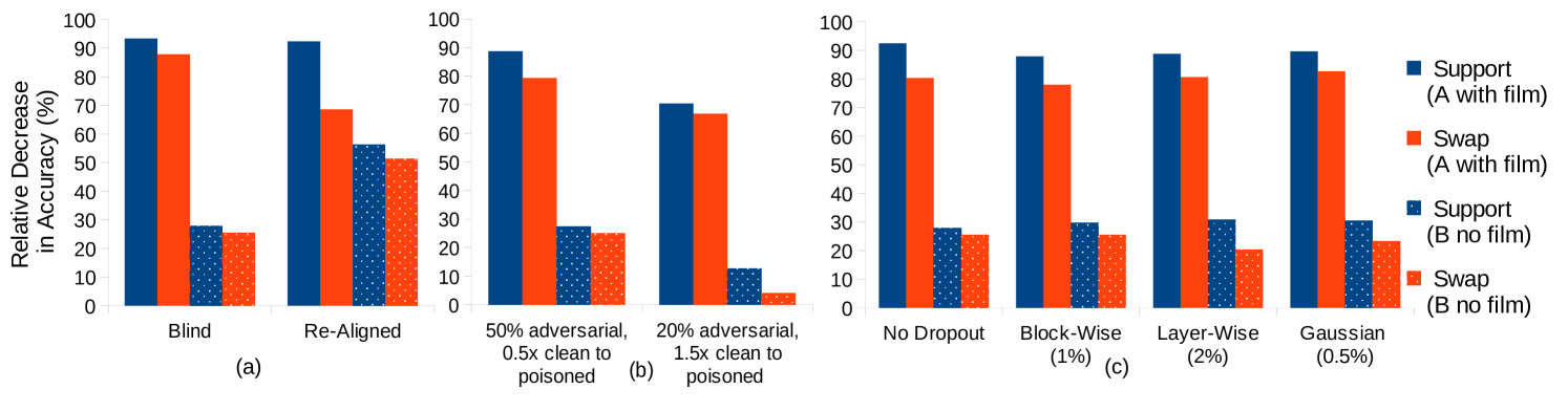
As shown in Fig.˜3(a), relabeling the support set does significantly improve transfer compared to the “blind” scenario in which the surrogate model has no knowledge about the target model’s decision boundaries. However, ASP is still not significantly better than the swap attack.
Hot Start
The ASP optimization procedure may be finding a different minimum, which is less robust to different feature extractors than that found by the swap attack. We propose to hot-start the ASP attack, where given a support set , we spend half the optimization budget performing a query attack to produce , which is then used as input to an adversarial support set attack to produce with the other half of the budget. In this way, we start the ASP attack off in the region of the local minimum found by the query attack. However, as shown in Fig.˜1, the hot start does not improve on the normally initialized ASP attack and may be worse in some scenarios.
Support Set Shuffling
Simple CNAPs makes use of a set encoder to produce a representation of the entire support set and so the attack must effectively manipulate the poisoned examples so that the embedded representation of the poisoned support set is sufficiently different to affect predictions. This may explain why we observe that the poisoning attack requires a high proportion of poisoned examples in the support set in order to be effective. The potency of the poisoned examples thus depend on the rest of the (unperturbed) support set. When transferred, the support set may embed very differently, especially if a large proportion of it is not adversarial, negating the effects of the poisoned points. In order to generate solutions that are less dependent on the rest of the support set we propose a procedure whereby the clean elements in the support set are not kept fixed for the duration of attack generation, but instead shuffle different clean images in and out of the support set. Fig.˜3(b) considers two configurations: each varying the percentage of the support set that is poisoned (50% and 20%, respectively) and the proportion of clean images in the support set during attack generation (the clean : poisoned ratio is and , respectively). Note that we are careful not to assume access to more data than any of the other scenarios. The first setting performs no better than an attack generated without shuffling. The second setting performs worse – although the attack has access to a more varied support set, this comes at the price of poisoning a smaller proportion of the support set since we cannot access additional data.
Dropout
If the attack optimization procedure is overfitting to the surrogate model, then regularization by dropout is an established remedy. By applying dropout to the feature extractor, we may hope for the resulting attack to generalize better to new feature extractors. We drop out the FiLM parameters of the surrogate’s feature extractor using one of three different strategies: (1) Block-Wise - the FiLM parameters for an entire Resnet block is either on/off, i.e. either computed as usual or we set , ; (2) Layer-Wise - each FiLM layer within a Resnet block may be switched on or off individually, i.e. compute and as usual, but apply a dropout mask; (3) Gaussian Dropout - the FiLM parameters are smoothed by a Gaussian with standard deviation given by where is the dropout probability. Although Fig.˜3(c) shows slight improvement in transferability, the difference between the ASP and swap attacks remain statistically insignificant.
5 Conclusion
In this paper, we propose ASP, an attack against amortized meta-learners that jointly crafts sets of colluding points which can manipulate a meta-learner when used as training data. We expect ASP attacks to be strong because the attack images are generated by backpropagating through the learner’s adaptation process with respect to the loss over an entire set of test inputs and are thus able to collude to fool the classifier. We may also expect ASP enjoy the same robustness to different feature extractors as a standard evasion attack. We show that although ASP is very effective in a white box setting, it does not transfer well, even to the same learner with a different feature extractor.
We explore a number of strategies to improve the transferability of ASP, but in all cases ASP was not able to transfer significantly better than the swap attack baseline (which performs a query or evasion attack in the usual way and simply swaps it into the meta-learner’s support set). Even though the swap attack should be much weaker, since it is generated to fool the learner only for the image in question, it proves a very effective baseline for poisoning few-shot learners. Since an attacker will rarely have access to the internal workings of the target model, the transferability of an attack is an important consideration, which prevents the deployment of ASP in real-life. But future work may glean insight into making models more robust.
Acknowledgments and Disclosure of Funding
This work was performed using resources provided by the Cambridge Service for Data Driven Discovery (CSD3) operated by the University of Cambridge Research Computing Service (www.csd3.cam.ac.uk), provided by Dell EMC and Intel using Tier-2 funding from the Engineering and Physical Sciences Research Council (capital grant EP/T022159/1), and DiRAC funding from the Science and Technology Facilities Council (www.dirac.ac.uk).
Richard E. Turner is supported by funding from Google, Amazon, ARM, Improbable and Microsoft. The paper built on software developed under Prosperity Partnership EP/T005386/1 between Microsoft Research and the University of Cambridge.
References
- Bateni et al. (2020) Peyman Bateni, Raghav Goyal, Vaden Masrani, Frank Wood, and Leonid Sigal. Improved few-shot visual classification. In Conference on Computer Vision and Pattern Recognition (CVPR), 2020.
- Biggio and Roli (2017) Battista Biggio and Fabio Roli. Wild patterns: Ten years after the rise of adversarial machine learning. CoRR, abs/1712.03141, 2017. URL http://arxiv.org/abs/1712.03141.
- Biggio et al. (2017) Battista Biggio, Igino Corona, Davide Maiorca, Blaine Nelson, Nedim Srndic, Pavel Laskov, Giorgio Giacinto, and Fabio Roli. Evasion Attacks against Machine Learning at Test Time. arXiv e-prints, art. arXiv:1708.06131, August 2017.
- Carlini and Wagner (2017) Nicholas Carlini and David Wagner. Towards evaluating the robustness of neural networks. In 2017 IEEE Symposium on Security and Privacy (SP), pages 39–57, May 2017. doi: 10.1109/SP.2017.49.
- Chen et al. (2017) Pin-Yu Chen, Yash Sharma, Huan Zhang, Jinfeng Yi, and Cho-Jui Hsieh. EAD: Elastic-Net Attacks to Deep Neural Networks via Adversarial Examples. arXiv e-prints, art. arXiv:1709.04114, Sep 2017.
- Finn et al. (2017) Chelsea Finn, Pieter Abbeel, and Sergey Levine. Model-agnostic meta-learning for fast adaptation of deep networks. In Doina Precup and Yee Whye Teh, editors, Proceedings of the 34th International Conference on Machine Learning, volume 70 of Proceedings of Machine Learning Research, pages 1126–1135, International Convention Centre, Sydney, Australia, 06–11 Aug 2017. PMLR. URL http://proceedings.mlr.press/v70/finn17a.html.
- Goldblum et al. (2019) Micah Goldblum, Liam Fowl, and Tom Goldstein. Adversarially robust few-shot learning: A meta-learning approach. arXiv, pages arXiv–1910, 2019.
- Goodfellow et al. (2014) Ian J Goodfellow, Jonathon Shlens, and Christian Szegedy. Explaining and harnessing adversarial examples. arXiv preprint arXiv:1412.6572, 2014.
- Gordon et al. (2019) Jonathan Gordon, John Bronskill, Matthias Bauer, Sebastian Nowozin, and Richard Turner. Meta-learning probabilistic inference for prediction. In International Conference on Learning Representations, 2019. URL https://openreview.net/forum?id=HkxStoC5F7.
- Ha et al. (2016) David Ha, Andrew Dai, and Quoc V Le. Hypernetworks. In International Conference on Learning Representations, 2016. URL https://openreview.net/forum?id=rkpACe1lx.
- Hospedales et al. (2020) Timothy Hospedales, Antreas Antoniou, Paul Micaelli, and Amos Storkey. Meta-learning in neural networks: A survey. arXiv preprint arXiv:2004.05439, 2020.
- Jagielski et al. (2018) Matthew Jagielski, Alina Oprea, Battista Biggio, Chang Liu, Cristina Nita-Rotaru, and Bo Li. Manipulating machine learning: Poisoning attacks and countermeasures for regression learning. In 2018 IEEE Symposium on Security and Privacy (SP), pages 19–35, 2018.
- Kim et al. (2017) Mijung Kim, Jasper Zuallaert, and Wesley De Neve. Few-shot learning using a small-sized dataset of high-resolution fundus images for glaucoma diagnosis. In Proceedings of the 2nd International Workshop on Multimedia for Personal Health and Health Care, MMHealth ’17, page 89–92, New York, NY, USA, 2017. Association for Computing Machinery. ISBN 9781450355049. doi: 10.1145/3132635.3132650. URL https://doi.org/10.1145/3132635.3132650.
- Krizhevsky and Hinton (2009) Alex Krizhevsky and Geoffrey Hinton. Learning multiple layers of features from tiny images. Technical report, Citeseer, 2009.
- Krizhevsky et al. (2012) Alex Krizhevsky, Ilya Sutskever, and Geoffrey E Hinton. Imagenet classification with deep convolutional neural networks. In Advances in neural information processing systems, pages 1097–1105, 2012.
- LeCun et al. (2010) Yann LeCun, Corinna Cortes, and CJ Burges. MNIST handwritten digit database. AT&T Labs [Online]. Available: http://yann. lecun. com/exdb/mnist, 2:18, 2010.
- Madry et al. (2017) Aleksander Madry, Aleksandar Makelov, Ludwig Schmidt, Dimitris Tsipras, and Adrian Vladu. Towards Deep Learning Models Resistant to Adversarial Attacks. arXiv e-prints, art. arXiv:1706.06083, June 2017.
- Mahajan et al. (2020) Kushagra Mahajan, Monika Sharma, and Lovekesh Vig. Meta-dermdiagnosis: Few-shot skin disease identification using meta-learning. In Proceedings of the IEEE/CVF Conference on Computer Vision and Pattern Recognition (CVPR) Workshops, June 2020.
- Newsome et al. (2006) James Newsome, Brad Karp, and Dawn Song. Paragraph: Thwarting signature learning by training maliciously. In Diego Zamboni and Christopher Kruegel, editors, Recent Advances in Intrusion Detection, pages 81–105, Berlin, Heidelberg, 2006. Springer Berlin Heidelberg. ISBN 978-3-540-39725-0.
- Papernot et al. (2016a) Nicolas Papernot, Patrick McDaniel, and Ian Goodfellow. Transferability in Machine Learning: from Phenomena to Black-Box Attacks using Adversarial Samples. arXiv e-prints, art. arXiv:1605.07277, May 2016a.
- Papernot et al. (2016b) Nicolas Papernot, Patrick McDaniel, Ian Goodfellow, Somesh Jha, Z. Berkay Celik, and Ananthram Swami. Practical Black-Box Attacks against Machine Learning. arXiv e-prints, art. arXiv:1602.02697, February 2016b.
- Perez et al. (2018) Ethan Perez, Florian Strub, Harm De Vries, Vincent Dumoulin, and Aaron Courville. FiLM: Visual reasoning with a general conditioning layer. In Thirty-Second AAAI Conference on Artificial Intelligence, 2018.
- Ravi and Larochelle (2017) Sachin Ravi and Hugo Larochelle. Optimization as a model for few-shot learning. In Proceedings of the International Conference on Learning Representations, 2017. URL https://openreview.net/pdf?id=rJY0-Kcll.
- Requeima et al. (2019a) James Requeima, Jonathan Gordon, John Bronskill, Sebastian Nowozin, and Richard E Turner. Fast and flexible multi-task classification using conditional neural adaptive processes. In H. Wallach, H. Larochelle, A. Beygelzimer, F. dÁlché-Buc, E. Fox, and R. Garnett, editors, Advances in Neural Information Processing Systems 32, pages 7957–7968. Curran Associates, Inc., 2019a.
- Requeima et al. (2019b) James Requeima, Jonathan Gordon, John Bronskill, Sebastian Nowozin, and Richard E Turner. Code for "Fast and flexible multi-task classification using conditional neural adaptive processes". https://github.com/cambridge-mlg/cnaps, 2019b.
- Rubinstein et al. (2009) Benjamin I.P. Rubinstein, Blaine Nelson, Ling Huang, Anthony D. Joseph, Shing-hon Lau, Satish Rao, Nina Taft, and J. D. Tygar. Antidote: Understanding and defending against poisoning of anomaly detectors. In Proceedings of the 9th ACM SIGCOMM Conference on Internet Measurement, IMC ’09, page 1–14, New York, NY, USA, 2009. Association for Computing Machinery. ISBN 9781605587714. doi: 10.1145/1644893.1644895. URL https://doi.org/10.1145/1644893.1644895.
- Russakovsky et al. (2015) Olga Russakovsky, Jia Deng, Hao Su, Jonathan Krause, Sanjeev Satheesh, Sean Ma, Zhiheng Huang, Andrej Karpathy, Aditya Khosla, Michael Bernstein, et al. Imagenet large scale visual recognition challenge. International journal of computer vision, 115(3):211–252, 2015.
- Sheryl Zhang et al. (2019) Xi Sheryl Zhang, Fengyi Tang, Hiroko Dodge, Jiayu Zhou, and Fei Wang. MetaPred: Meta-Learning for Clinical Risk Prediction with Limited Patient Electronic Health Records. arXiv e-prints, art. arXiv:1905.03218, May 2019.
- Snell et al. (2017) Jake Snell, Kevin Swersky, and Richard Zemel. Prototypical networks for few-shot learning. In I. Guyon, U. V. Luxburg, S. Bengio, H. Wallach, R. Fergus, S. Vishwanathan, and R. Garnett, editors, Advances in Neural Information Processing Systems 30, pages 4077–4087. Curran Associates, Inc., 2017.
- Szegedy et al. (2014) Christian Szegedy, Google Inc, Wojciech Zaremba, Ilya Sutskever, Google Inc, Joan Bruna, Dumitru Erhan, Google Inc, Ian Goodfellow, and Rob Fergus. Intriguing properties of neural networks. In In ICLR, 2014.
- Triantafillou et al. (2020) Eleni Triantafillou, Tyler Zhu, Vincent Dumoulin, Pascal Lamblin, Utku Evci, Kelvin Xu, Ross Goroshin, Carles Gelada, Kevin Swersky, Pierre-Antoine Manzagol, and Hugo Larochelle. Meta-dataset: A dataset of datasets for learning to learn from few examples. In International Conference on Learning Representations, 2020. URL https://openreview.net/forum?id=rkgAGAVKPr.
- Vinyals et al. (2016) Oriol Vinyals, Charles Blundell, Timothy Lillicrap, koray kavukcuoglu, and Daan Wierstra. Matching networks for one shot learning. In D. D. Lee, M. Sugiyama, U. V. Luxburg, I. Guyon, and R. Garnett, editors, Advances in Neural Information Processing Systems 29, pages 3630–3638. Curran Associates, Inc., 2016.
- Yin et al. (2018) Chengxiang Yin, Jian Tang, Zhiyuan Xu, and Yanzhi Wang. Adversarial meta-learning. arXiv preprint arXiv:1806.03316, 2018.
Appendix A Appendix
A.1 Episodic Training
There has been an explosion of meta-learning based few-shot learning algorithms proposed in recent years. For an in-depth review see Hospedales et al. [2020]. The majority of modern meta-learning methods employ episodic training [Vinyals et al., 2016]. During meta-training, a task is drawn from and randomly split into a support set and query set . Fig.˜4 depicts an example few-shot classification task.
The meta-learner takes as input the support set and produces task-specific classifier parameters which are used to adapt the classifier to the current task. The classifier can now make task-specific predictions for any test input . Refer to Clean in Fig.˜5. A loss function then computes the loss between the predictions for the label and the true label . Assuming that , , and are differentiable, the meta-learning algorithm can then be trained with stochastic gradient descent by back-propagating the loss and updating the parameters of and .
A.2 Few-shot Learner Meta-training Protocols
In the following, the meta-training protocols for the few-shot learners used in the experiments.
A.2.1 Datasets
miniImageNet
miniImageNet is a subset of the larger Imagenet dataset [Russakovsky et al., 2015] created by Vinyals et al. [2016]. It consists of 60,000 color images that is sub-divided into 100 classes, each with 600 instances. The images have dimensions of pixels. Ravi and Larochelle [2017] standardized the 64 training, 16 validation, and 20 test class splits. miniImageNet has become a defacto standard dataset for benchmarking few-shot image classification methods with the following classification task configurations: 1 5-way, 1-shot; 2 5-way, 5-shot.
Meta-Dataset
Meta-Dataset [Triantafillou et al., 2020] is composed of ten (eight train, two test) image classification datasets. We augment Meta-Dataset with three additional held-out datasets: MNIST [LeCun et al., 2010], CIFAR10 [Krizhevsky and Hinton, 2009], and CIFAR100 [Krizhevsky and Hinton, 2009]. The challenge constructs few-shot learning tasks by drawing from the following distribution. First, one of the datasets is sampled uniformly; second, the “way” and “shot” are sampled randomly according to a fixed procedure; third, the classes and support / query instances are sampled. Where a hierarchical structure exists in the data (ImageNet or Omniglot), task-sampling respects the hierarchy. In the meta-test phase, the identity of the original dataset is not revealed and the tasks must be treated independently (i.e. no information can be transferred between them). Notably, the meta-training set comprises a disjoint and dissimilar set of classes from those used for meta-test. Meta-Dataset is presently, the "gold standard" for evaluating few-shot classification methods. Full details are available in Triantafillou et al. [2020].
In our experiments, we excluded the Omniglot, Textures, Fungi, and Traffic Signs datasets from evaluation because their test splits are too small to allow for a fair assessment of the attack’s generalization, even though the attacks reduced the classification accuracy on those datasets to approximately zero in the ASP Specific case.
For Meta-Dataset, we meta-trained Simple CNAPs using the code from Requeima et al. [2019b] with FiLM feature adaptation. We made modifications to the code to enable various adversarial attacks. The meta-trained model attained the following results:
ilsvrc 2012: , omniglot: , aircraft: , cu birds: , dtd: , quickdraw: , fungi: , vgg flower: , traffic sign: , mscoco: , mnist: , cifar10: , cifar100: .
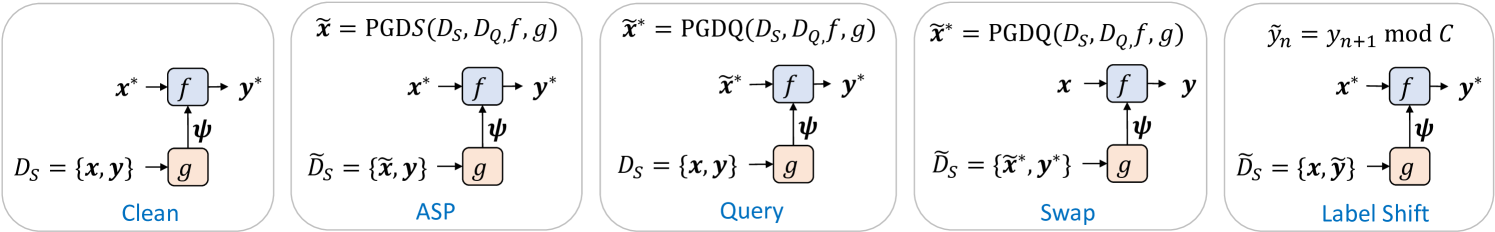
A.3 Attack Summary
We summarize the types of attacks we perform in Fig.˜5. The first scenario, Clean, illustrates how the meta-learner performs a test-time task, taking the support set as input to produce parameters which are used to adapt the classifier to the task. The classifier makes task-specific predictions for any test input . ASP and Query illustrate the ASP and Query attacks as discussed in Section˜3. Swap illustrates a swap attack, which is used as a baseline comparison for ASP, where a set of images are perturbed with a query attack and then inserted into the support set. Query attacks are typically cheaper to compute, since they do not require back-propagation through the meta-learner, so it is an important baseline to consider.
A.4 Additional Experimental Details
In our experiments, all the input images were re-scaled to have pixel values between and . We considered perturbations using the norm, on a scale of , so that corresponds to allowing or an absolute change of to the intensity of each pixel in an image.
We calculated the perturbation step size to depend on and the maximum number of iterations, so that , where is a scaling coefficient.
A.5 Unnormalised Large-Scale Attack Results
This section of the appendix presents the unnormalized results for all figures, along with 95% confidence intervals.
In Table˜1 we present the unnormalized numbers for Fig.˜1, which shows the efficacy of ASP in a white box setting. Table˜2 considers transfer between a surrogate model and target models with different feature extractors as presented in Fig.˜2(Left). Tables 3 and 4 consider the effect of the hot-start mitigation strategy for different perturbation sizes as presented in Fig.˜2(Right). Tables 5, 6 and 7 correspond to Fig.˜3 and show the effect of other mitigation strategies, specifically decision boundary re-alignment, shuffling different clean inputs into the support set, and dropout. All numbers are percentages and the sign indicates the 95% confidence interval.
Clean Specific General Swap ilsvrc_2012 52.20.2 1.50.1 14.80.1 42.80.2 aircraft 78.50.5 0.00.0 7.20.2 65.31.0 cu_birds 71.41.1 1.80.2 8.90.4 50.62.0 quickdraw 74.10.1 32.81.2 41.30.2 57.70.3 vgg_flower 89.10.6 10.60.8 27.71.0 78.71.8 traffic_sign 35.20.4 4.10.3 12.30.3 24.80.5 mscoco 44.10.3 2.90.1 10.80.1 29.20.3 mnist 90.30.1 58.81.4 68.90.2 85.80.2 cifar10 64.60.1 1.60.1 13.50.1 51.80.2 cifar100 53.50.6 2.40.1 7.70.2 25.00.8
Clean ASP Swap Surrogate Scenario A 52.42.1 3.60.4 2.90.4 (Resnet A FiLM) Scenario B 54.21.2 3.20.2 4.90.3 Scenario C 54.51.8 3.60.3 6.60.6 Transfer to Scenario A 48.72.1 4.70.5 3.90.5 Resnet A (no FiLM) Scenario B 50.21.2 4.60.3 4.00.3 Scenario C 50.53.4 32.72.0 28.21.3 Transfer to Scenario A 38.62.0 4.90.6 4.60.6 Resnet B (no FiLM) Scenario B 39.11.2 10.20.6 9.00.5 Scenario C 40.11.9 28.92.0 29.91.6
Clean ASP Swap Hot Start Surrogate (Resnet18 A no FiLM) 52.10.7 20.10.4 46.30.9 22.00.4 Transfer to Resnet18 A (with FiLM) 55.80.7 31.50.7 28.70.5 35.20.7 Transfer to Resnet18 B (no FiLM) 43.60.7 36.10.7 32.20.6 36.40.7
Clean ASP Swap Hot Start Surrogate (Resnet18 A no FiLM) 54.10.8 16.00.4 50.90.8 16.10.4 Transfer to Resnet18 A (with FiLM) 58.10.8 46.20.8 41.10.7 48.50.8 Transfer to Resnet18 B (no FiLM) 45.70.7 41.80.7 35.70.6 43.10.7
Clean ASP Swap Surrogate Re-Aligned 52.62.0 4.00.4 16.51.9 (Resnet18 A with FiLM) Blind 54.51.8 3.60.3 6.60.6 Transfer to Re-Aligned 43.92.1 19.21.2 21.40.9 Resnet18 B (no FiLM) Blind 40.11.9 28.92.0 29.91.6
Clean ASP Swap Surrogate Setting A 55.72.2 6.30.6 11.51.3 (Resnet18 A with FiLM) Setting B 68.80.4 32.40.4 44.60.7 Transfer to Setting A 41.32.1 30.02.1 31.01.5 Resnet18 B (no FiLM) Setting B 55.10.4 51.70.5 48.40.3
Surrogate (Resnet18 A with FiLM) Transfer to Resnet18 B (no FiLM) Clean ASP Swap Clean ASP Swap No dropout 55.51.4 4.20.3 10.91.1 40.11.9 28.92.0 29.91.6 Block-Wise (1%) 44.61.5 5.40.3 9.80.7 42.31.8 29.71.8 31.51.3 Layer-Wise (2%) 44.52.1 5.00.5 8.61.0 38.31.9 26.51.8 30.51.5 Gaussian (0.5%) 47.41.6 4.90.4 8.21.0 39.01.5 27.11.4 29.91.2
A.6 Query Attacks
We present our algorithm for performing query attacks with PGD in Algorithm˜2.