Adversarial Defense via Image Denoising with Chaotic Encryption
Abstract
In the literature on adversarial examples, white box and black box attacks have received the most attention. The adversary is assumed to have either full (white) or no (black) access to the defender’s model. In this work, we focus on the equally practical gray box setting, assuming an attacker has partial information. We propose a novel defense that assumes everything but a private key will be made available to the attacker. Our framework uses an image denoising procedure coupled with encryption via a discretized Baker map. Extensive testing against adversarial images (e.g. FGSM, PGD) crafted using various gradients shows that our defense achieves significantly better results on CIFAR-10 and CIFAR-100 than the state-of-the-art gray box defenses in both natural and adversarial accuracy.
1 Introduction
For our AI systems to be considered safe, we must ensure that they can withstand attacks from adversaries. Unfortunately, most machine learning models are vulnerable to these attacks (Szegedy et al., 2014). Consider the task of autonomous driving. These systems can not only be attacked virtually, by directly manipulating inputs such as pixels, but they can also be attacked by altering the physical world. For instance, Eykholt et al. (2018) show that stop signs can be erroneously classified as speed limit signs simply by placing a small patch on the sign.
Protecting our systems from such attacks is made especially challenging when there is a need for real-time decision making. Again consider a vision system for an autonomous vehicle. Since objects on the road must be detected as quickly as possible, there is no time to communicate with a cloud service, and the classifier must be located in on-device memory. Hence, an adversary will have direct access to the on-device model, allowing them to craft adversarial examples quite easily (Kurakin et al., 2017). To address these cases, we must develop safety methodologies that assume the model is visible to the attacker.
We propose a novel gray box adversarial defense that assumes everything but a private key will be made available to the attacker. We accomplish this by using an image denoising procedure coupled with encryption via a discretized Baker map (Fridrich, 1998). The encryption key is what we must keep secret from the attacker. For a sketch of our approach, Figure 1 demonstrates the Baker map encryption, and Figure 2 shows a diagram of our proposed method. We evaluate our defense against two gradient-based adversarial attacks: the Fast Gradient Sign Method (Goodfellow et al., 2015) and Projected Gradient Descent (Madry et al., 2018). We achieve significantly better results than state-of-the-art gray box defenses in both natural and adversarial accuracy.


2 Setting of Interest: Gray Box Attacks
Notation
Throughout the paper, let denote an image, its true label, a classifier, an image denoiser, k an encryption key, and an image encryption and its decryption algorithm, and a loss function (e.g., the cross-entropy loss). We abbreviate as , Fast Gradient Sign Method as FGSM, and Projected Gradient Descent as PGD. PGD- means PGD uses optimization steps.
We begin by defining the classes of adversarial attacks: white, gray, and black box. The distinguishing characteristic is in how much information is assumed available to the attacker.
White Box The white box setting assumes that the attacker has access to the same information as the defender, including the model parameters, training data, and the defense mechanism (e.g., adversarial training (Goodfellow et al., 2015)). This setting places the most burden on the efficacy of the defense mechanism, with the upside being that there is no need to keep information private upon deployment.
Gray Box The gray box setting assumes that only partial information about the model is available to the attacker. The inaccessible data can include the trainable parameters and an encryption key (Taran et al., 2019). In this paper, we assume the key is always private (if it is used), and further subdivide the gray box attacks into dark, medium and light types, where the trainable parameters are completely inaccessible, partially inaccessible, and completely accessible.
Black Box The black box setting assumes that all information about the model is unknown to the attacker. The attacker can proceed only by training a surrogate model using the target model’s outputs as labels (Papernot et al., 2017). This setting places the most burden on the system’s security since all information must be protected. If the attacker is able to bypass this security and access the model, then it will be easy to degrade the system’s performance since no other protections are in place.
Motivation
In this paper, we focus on the gray box setting. The white box and black box settings have attracted the most attention in the literature. In comparison, gray box attacks are under-explored yet are still germane to many modern technologies. Returning to the self-driving car example, the car manufacturer is free to publish (via software update) their architecture and/or defense mechanism without a concern for security, as long as the designated private information is kept as such (e.g. encryption key). In our approach, the private information will be an encryption key, which should be easier to keep private than the parameters of a large neural network.
Our proposed method is inspired by the limitations of previously proposed denoising- and encryption-based gray box approaches. For an example of the former, Liao et al. (2018) train a classifier () using natural images, then use the U-net (Ronneberger et al., 2015) as a denoising model () to protect against the adversarial images crafted using the gradient . This defense mechanism achieves good natural and FGSM accuracy (Liao et al., 2018). Unfortunately, Athalye & Carlini (2018) show that it is vulnerable to PGD attacks crafted using the end-to-end gradient (we note (Liao et al., 2018) was proposed as a white box defense, but their vulnerability to PGD attacks remains in the gray box setting). For an example of the latter, Taran et al. (2019) encrypt the input images during training and testing. However, their method’s performance is still far from satisfactory in natural accuracy and real-world applications.
3 Method
We propose an encrypt-denoise-decrypt approach. In the first step, we encrypt the images via a public encryption algorithm with private key k. In the second step, the encrypted images are passed into a denoising model . We use the U-net for , following (Liao et al., 2018). The third step is to decrypt the denoised image: where denotes the final decypted and denoised image. Lastly, we feed to the classifier for prediction. Below we discuss the encryption and denoising procedures in more detail.
3.1 Chaotic Encryption
We need the encryption algorithm to meet two criterion. The first is that distinct keys must result in sufficiently different outputs. If many keys were to result in the same encrypted images, then the key need not be compromised for an attack to succeed. Rather, the attacker needs only to guess one of the equivalent keys. The second requirement is a result of using a CNN-based denoiser. Because CNNs operate by way of local correlations, the encryption algorithm must preserve the input’s local structure to some degree.
For our choice of the encryption algorithm , we use the discretized Baker map proposed by (Fridrich, 1998), version A. We consider only square images in this work, but the encryption can be extended to rectangular images (Fridrich, 1998). Further, if the image has multiple channels, we apply the same encryption to each channel. The key for the encryption is a small set of integers , where each is divisible by the image dimension , and their sum . Let us denote , where . Then, for the pixel at position at iteration , where and , we use the following equations to move it to the new position :
| (1) | ||||
| (2) |
The key partitions the image into vertical rectangles, each of shape . Further, each rectangle is partitioned into boxes, where each box has shape , and has thus exactly pixels. Next, we stretch the pixels in each box to a row of shape , then stack the rows together to produce the permuted image. Two examples of the encryption using keys and on a simple matrix are shown in Eqs. 11 and 20.
| (11) | ||||
| (20) |
The total number of possible keys depends on both the image dimension and the number of divisors of . In general, grows rapidly with . Table 1 shows a few examples of their relation, which suggests that it is highly unlikely that the attacker and defender can use the same key by chance.
| 16 | 5271 |
| 32 | |
| 64 | |
| 128 | |
| 256 | |
| 512 | |
| 1024 |
Let us examine the Baker map encrypted images in Figure 1. The figure shows that more encryption iterations leads to more random image patterns, where the local spatial relations in the input images are destroyed. However, with few iterations, some spatial relations are preserved and the resulting images have perceptible structures, yet different keys lead to noticeably different structures. These properties make the Baker map encryption ideally suited for our purposes, though it can be replaced by other viable encryption schemes for our defense.
3.2 Training Procedure
Our defense trains the classifier and the U-net denoiser in 2 steps. We first train the classifier using only natural images. After training, we fix its weights, and then train the denoiser using the encrypted adversarial inputs . The gradient for the adversarial perturbation comes from the trained classifier, which is . Let us denote as the feature map after the last convolution block of the classifier, our training loss for the denoiser is:
| (21) |
where . Namely, we minimize the distances between the denoised and natural images and , as well as the last convolution feature maps for the two images. The second loss provides guidance to the first one, and the combined loss achieves much better results than the first loss alone.
Alternatively, we could feed the encrypted images directly to the classifier without the denoiser. If the input images have simple structures such as MNIST, then feeding the permuted images to a CNN-based classifier barely reduces the natural accuracy; however, as the complexity of the dataset grows, classifying the permuted images leads to increasingly lower accuracy compared to the unpermuted counterpart (Ivan, 2019). Using the U-net denoiser with image encryption and decryption alleviates this problem: though the U-net is still CNN-based, the denoised images are decrypted (i.e., permuted back) to the original pixel order before being fed to the classifier, which improves the accuracy. Further, since the denoiser is trained only to denoise images, the attacker cannot easily deduce the private key even if they can access the denoiser’s weights. In comparison, if the denoiser learns to both denoise and decrypt images, then it is possible that the attacker can recover the private key by feeding it with inputs of simple patterns (e.g., an image that contains a single non-zero column), and observing the pixel orders in the outputs.
3.3 Adversarial Attacks
In gray box attacks, the defender’s key generator and model architecture are public, but their random seed is assumed to be different from the attacker’s. Thus, their generated private keys and initial model weights are different.
In testing, the defender’s model with the private key k can be attacked by the adversarial images crafted using the 4 gradients listed below. To compute these gradients, the attacker uses the defender’s classifier’s weights if their are public; otherwise, the attacker trains their classifier initialized using their random seed.
-
1.
The gradient from the classifier: .
-
2.
The end-to-end gradient without encryption: attacker trains their denoiser using unencrypted images, and obtains the gradient .
-
3.
The end-to-end gradient with encryption using the key for training: the attacker trains their denoiser using encrypted images with their key , and obtains the gradient .
-
4.
The end-to-end gradient with encryption using random keys. This is similar to gradient 3, except in testing, rather than using the same key for training, the attacker samples a random key for FGSM, and each step of PGD- (i.e., there are keys for PGD-). Thus, if the defender’s denoiser’s weights are public, then the attacker obtains the gradient . Otherwise, the attacker trains their denoiser using the encrypted images with their key , and obtains the gradient .
4 Experiments
We use the original ResNet-18 classifier (He et al., 2016), and the CIFAR-10 and CIFAR-100 datasets (Krizhevsky & Hinton, 2009) with the original image dimensions . For natural training (i.e., the classifier is trained using only natural images), we use the same training procedure as (Madry et al., 2018), which augments the training inputs using cropping and horizontal flipping, and optimizes the model using stochastic gradient descent (SGD) for 200 epochs. The learning rate starts at , and decays to and after 100 and 150 epochs. This achieves 95.28% and 75.55% test accuracy on natural CIFAR-10 and CIFAR-100 images respectively.
We use two gradient-based adversarial attacks in norm, which are FGSM and PGD-. FGSM is an one-step attack, and the adversarial image is a point on the boundary of a small norm ball centered at in the direction of the sign of the gradient:
| (22) |
In comparison, PGD- is a multi-step attack, which starts at a random point within the norm ball centered at , and runs steps. In each step , it finds a point within that maximizes the loss with the step size :
| (23) |
For both attacks, the radius of the norm ball ; for PGD-, the step size . We use the CleverHans (Papernot et al., 2018) implementation in PyTorch (Paszke et al., 2019)111https://github.com/cleverhans-lab/cleverhans to craft the adversarial images, and compare with two adversarial defenses, which are adversarial training and multi-channel sign permutation. The former is one of the few unbroken defenses to this day, and the latter is an existing state-of-the-art gray box defense with an encryption key.
4.1 Adversarial Training
In adversarial training (Goodfellow et al., 2015; Madry et al., 2018), the defender trains the classifier using adversarial images. For each natural image and its label , this defense first creates the adversarial image using FGSM (Eq. 22) or PGD- (Eq. 23), then updates the classifier’s weights using the input and label . In the experiments, we use PGD-7 for the training inputs. We also tried PGD-20 as the inputs, and found the results are very similar to that of PGD-7, but training takes much longer. Lastly, we train the classifier using the same procedure as for natural training.
4.2 Multi-Channel Sign Permutation
Taran et al. (2019) propose an encryption-based defense mechanism, which first transforms the input image using the public discrete cosine transform (DCT) , then multiplies it with a secret sign permutation matrix , and finally transforms it back to the image domain using the inverse DCT . There are possible DCT sub-bands, which are vertical (V), horizontal (H) and diagonal (D), and channels per sub-band. For each channel, it performs the encryption as , where , then classifies the encrypted image using a convolutional network . Lastly, it averages over the outputs of all channels to make the final prediction .
For the experiments, we follow the same test setup as in Table 2 of their paper. Namely, we use all 3 sub-bands V, H and D, and increase the number of channels per sub-band I from 1 to 5. The total number of channels is thus 3, 6, 9, 12 or 15. Lastly, we use the same implementation released by the authors222https://github.com/taranO/defending-adversarial-attacks-by-RD, but re-implement the code in PyTorch to be consistent with other methods.
4.3 Our Defense
We use an existing implementation for the U-net denoiser by Zbontar et al. (2018)333https://github.com/facebookresearch/fastMRI/blob/14562052eb3f37dd1f23f694bddfc3b8d456d571/models/unet/unet_model.py. It has 4 convolution blocks, the number of output channels of the first convolution layer is 128, and dropout (Srivastava et al., 2014) is not used. Further, we randomly choose the FGSM and PGD-7 adversarial images as its input with equal probabilities. We found that alternating the two types of inputs achieves better overall adversarial accuracy compared to using just one of them. However, for adversarial training, using the PGD-7 inputs alone works better. Lastly, we optimize the denoiser using the same procedure as for the classifier, but we do not use input augmentations.
4.4 Results
4.4.1 Dark Gray Box Defense
| Defense | CIFAR-10 | CIFAR-100 | ||||||
|---|---|---|---|---|---|---|---|---|
| Natural | FGSM | PGD-7 | PGD-20 | Natural | FGSM | PGD-7 | PGD-20 | |
| Natural training | 95.28 | 47.15 | 10.01 | 7.11 | 75.55 | 18.67 | 11.82 | 9.97 |
| Adversarial training | 84.74 | 72.17 | 71.26 | 70.16 | 56.47 | 46.86 | 46.87 | 46.12 |
| Taran et al. () | 80.89 | 60.61 | 56.28 | 50.05 | 46.56 | 39.04 | 42.08 | 40.25 |
| Taran et al. () | 83.08 | 55.58 | 48.87 | 43.10 | 50.37 | 40.26 | 43.37 | 40.41 |
| Taran et al. () | 83.34 | 52.34 | 45.60 | 41.09 | 51.69 | 39.77 | 41.62 | 37.97 |
| Taran et al. () | 83.89 | 50.68 | 44.12 | 39.68 | 52.59 | 37.99 | 40.18 | 35.74 |
| Taran et al. () | 83.94 | 50.03 | 43.35 | 39.05 | 53.06 | 36.67 | 38.18 | 33.81 |
| Ours (without encryption) | 93.58 | 81.15 | 64.78 | 62.37 | 70.42 | 53.72 | 49.05 | 44.46 |
| Ours (with encryption) | 92.43 | 78.96 | 83.32 | 77.87 | 70.09 | 55.95 | 61.32 | 59.40 |
For dark gray box attacks, the adversary does not have access to the defender’s model parameters or key. Thus, they use the same training data and procedure to train an identical model with their initialization seed, then use the gradient of this model to craft the adversarial images444We note that Madry et al. (2018) refer to this setting as the “black box” attack.. Table 2 compares the test accuracy on CIFAR-10 and CIFAR-100. As a reference, we also show the test results for natural training. Unsurprisingly, it achieves the highest accuracy on natural images, but lowest on adversarial images. In comparison, adversarial training markedly improves the adversarial accuracy, but comes with a considerable cost for natural accuracy. For Taran et al., as the total number of channels increases from 3 to 15, the natural accuracy slowly increases, but all adversarial accuracies decrease. In addition, none of the configurations achieves better results than adversarial training. Its natural accuracy is comparable with adversarial training, since the encryption method does not significantly alter the appearance of the input images555This is illustrated in Figure 6 of (Taran et al., 2019).. Unfortunately, due to the same reason, the trained weights for the defender’s ensemble are not sufficiently different from the attacker’s, which makes the former vulnerable to the adversarial attacks.
For our method, we show the results without and with encryption. If encryption is not used, the defender feeds the inputs directly to the denoiser. Otherwise, they first choose a private key k for the Baker map, then feed the encrypted images to the denoiser. Since each type of adversarial image (FGSM, PGD-7 or PGD-20) can be crafted using one of the four gradients described in Section 3.3, we report the minimum accuracy of the four for each attack. This is because if the attacker knows the defender’s model, then they will use the most harmful gradient to craft the adversarial images. For these results, the defender’s key , and the attacker’s key for gradient 3 or 4 is . Both keys are randomly chosen.
Table 2 shows our defense significantly outperforms other defenses in both natural and adversarial accuracy. Particularly, our natural accuracy is close to the one obtained by natural training. Further, Figure 3 shows our individual adversarial accuracy against each gradient for each attack. In this figure, the top row shows that the model without encryption is especially vulnerable to the PGD end-to-end gradient without encryption (gradient 2). Here, the difference in the attacker’s and defender’s models is only their trained weights due to different weight initializations. In comparison, the bottom row shows that the model with encryption gains strong protection against all gradients.
These results lead to the following conclusions. First, initializing the model weights using a private seed provides moderate protection against adversarial attacks. Second, using a denoiser to remove the potential adversarial noise drastically improves the natural and FGSM accuracy. However, without encryption, this defense is still vulnerable to the PGD attacks. Third, in comparison, using encryption slightly affects the natural and FGSM accuracy, but significantly boosts the PGD accuracy by 12 to 19%.


4.4.2 Key Length

We discuss the impact of the defender’s key length on the gray box test accuracy, where . These keys are shown in Table 3, and they are randomly chosen. For 1 and 2, there is only one possible key. is a special case, since encrypting using the key is equivalent to the model without encryption. This means that the shortest key length for encryption is 2.
For these experiments, the attacker and defender initialize their models with different random seeds. We use the first three gradients in Section 3.3 to craft the adversarial images (for gradient 3, the attacker’s key is randomly chosen as ). To evaluate the benefit of the key, we include an additional case where the attacker and defender use the same key for each key length; this means their encrypted inputs are the same, and the difference is only their trained weights due to different weight initializations.
| Defender’s key | Key length |
|---|---|
| 4 | |
| 8 | |
| 12 |
Figure 4 shows that does not have a significant impact on our gray box test results with encryption. Further, if the defender’s key is different from the attacker’s (column 3), the adversarial accuracy is much better compared to the case when their keys are the same (column 4), which demonstrates the effectiveness of the key.
4.4.3 Light and Medium Gray Box Defenses
This section presents the test results when the defender’s classifier ’s weights are public. For adversarial training, this is equivalent to the white box defense, since the attacker can obtain the gradient directly from . In contrast, our defense is light or medium gray box since the key is private, so the attacker cannot obtain the end-to-end gradient directly from the defender’s model. Thus, it is not entirely fair to compare the results. Instead, our goal is to show that as more components in the defender’s model become private, the adversarial accuracy considerably improves. To attack our defense, the 4 gradients in Section 3.3 are used to craft the adversarial images, and our minimum accuracy is reported.
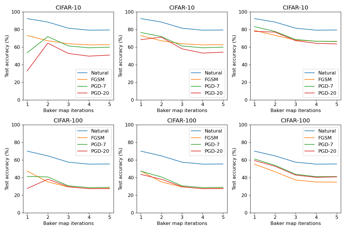

Figure 5 illustrates the test accuracy of our gray box defenses vs. the number of Baker map iterations. In general, as the iteration increases, the encrypted images become more random, and our performance decreases; the PGD accuracy at iteration 1 is an exception, which we will explain in the following text. Figure 6 shows that for our defense, when both the classifier’s and denoiser’s weights are public (i.e., light gray box), the performance is already much better than adversarial training, except for FGSM on CIFAR-100, which is slightly worse. Here, if we use only 1 Baker map iteration, the model is especially vulnerable to the PGD end-to-end gradient with encryption using random keys (gradient 4); namely, the attacker uses the defender’s model weights, and samples a random key for each PGD step. However, if 2 iterations are used, the method can effectively defend against gradient 4, although it comes with a small penalty for the natural and FGSM accuracy. We conjecture that by using 2 iterations, the defender’s encrypted inputs are sufficiently random, such that it is difficult for the attacker to sample similar inputs to craft the adversarial images. Meanwhile, when the denoiser’s weights are private (i.e., medium gray box), gradient 4 is no longer effective for the attack, so we use 1 Baker map iteration, and the results are better compared to the light gray box case. In sum, the defender’s performance improves as more model components become private.
5 Related Work
Our proposed method is a deterministic defense controlled by a random seed, and the seed determines the transformation of the inputs as well as the initialization of the model weights. Previous works such as (Buckman et al., 2018; Guo et al., 2018) use input transformations as a defense, but their goal is to shatter the gradient, such that the attacker cannot find the correct gradient to craft adversarial images. There are also defenses based on test-time randomization, such as (Xie et al., 2018; Dhillon et al., 2018), which ensure that the defender’s inputs and/or model weights are different from the attacker’s during inference. Unfortunately, Athalye et al. (2018) show that all these defenses can be broken by approximating the gradient for the defender’s model. In comparison, for our defense, unless the attacker knows the defender’s private seed, it is difficult to approximate the gradient due to the Baker map encryption and random weight initializations. Lastly, other interesting key-based gray box defenses include (Chen et al., 2019; Vinh et al., 2016).
6 Conclusion and Future Work
The previous literature on adversarial examples focused heavily on white box and black box attacks, but paid little attention to the equally practical gray box attacks. We propose a novel defense that assumes everything but a private key will be made available to the attacker. Our framework uses an image denoising procedure coupled with encryption via a discretized Baker map. Extensive testing against the FGSM and PGD adversarial images crafted using various gradients shows that we achieve significantly better results than the state-of-the-art gray box defenses in both natural and adversarial accuracy. Our method is easy to implement, suitable for high-resolution inputs, and efficient in testing.
To prevent the black box attacks where the attacker trains a surrogate model to mimic the behavior of defender’s, the defender can train an ensemble of denoisers, each using a different private key (the classifier is the same). Then, each time in testing, they randomly choose one denoiser from the ensemble to make the prediction. Since the total number of encryption keys is very large, it is infeasible for the attacker to train an ensemble of denoisers using all keys, and then use the mean gradient for the attack. We leave the verification of this idea for future work.
Acknowledgements
This research was supported by the NWO Perspective grant DLMedIA and the in-cash and in-kind contributions by Philips.
References
- Athalye & Carlini (2018) Athalye, A. and Carlini, N. On the robustness of the cvpr 2018 white-box adversarial example defenses. arXiv preprint arXiv:1804.03286, 2018.
- Athalye et al. (2018) Athalye, A., Carlini, N., and Wagner, D. Obfuscated gradients give a false sense of security: Circumventing defenses to adversarial examples. ICML, 2018.
- Buckman et al. (2018) Buckman, J., Roy, A., Raffel, C., and Goodfellow, I. Thermometer encoding: One hot way to resist adversarial examples. ICLR, 2018.
- Chen et al. (2019) Chen, Z., Tondi, B., Li, X., Ni, R., Zhao, Y., and Barni, M. Secure detection of image manipulation by means of random feature selection. IEEE Transactions on Information Forensics and Security, 2019.
- Dhillon et al. (2018) Dhillon, G. S., Azizzadenesheli, K., Lipton, Z. C., Bernstein, J., Kossaifi, J., Khanna, A., and Anandkumar, A. Stochastic activation pruning for robust adversarial defense. ICLR, 2018.
- Eykholt et al. (2018) Eykholt, K., Evtimov, I., Fernandes, E., Li, B., Rahmati, A., Xiao, C., Prakash, A., Kohno, T., and Song, D. Robust physical-world attacks on deep learning models. CVPR, 2018.
- Fridrich (1998) Fridrich, J. Symmetric ciphers based on two-dimensional chaotic maps. International Journal of Bifurcation and Chaos, 1998.
- Goodfellow et al. (2015) Goodfellow, I. J., Shlens, J., and Szegedy, C. Explaining and harnessing adversarial examples. ICLR, 2015.
- Guo et al. (2018) Guo, C., Rana, M., Cisse, M., and van der Maaten, L. Countering adversarial images using input transformations. ICLR, 2018.
- He et al. (2016) He, K., Zhang, X., Ren, S., and Sun, J. Deep residual learning for image recognition. CVPR, 2016.
- Ivan (2019) Ivan, C. Convolutional neural networks on randomized data. CVPR Workshops, 2019.
- Krizhevsky & Hinton (2009) Krizhevsky, A. and Hinton, G. Learning multiple layers of features from tiny images. Technical report, University of Toronto, 2009.
- Kurakin et al. (2017) Kurakin, A., Goodfellow, I., and Bengio, S. Adversarial examples in the physical world. arXiv preprint arXiv:1607.02533, 2017.
- Liao et al. (2018) Liao, F., Liang, M., Dong, Y., Pang, T., Hu, X., and Zhu, J. Defense against adversarial attacks using high-level representation guided denoiser. CVPR, 2018.
- Madry et al. (2018) Madry, A., Makelov, A., Schmidt, L., Tsipras, D., and Vladu, A. Towards deep learning models resistant to adversarial attacks. ICLR, 2018.
- Papernot et al. (2017) Papernot, N., McDaniel, P., Goodfellow, I., Jha, S., Celik, Z. B., and Swami, A. Practical black-box attacks against machine learning. ACM Asia Conference on Computer and Communications Security, 2017.
- Papernot et al. (2018) Papernot, N., Faghri, F., Carlini, N., Goodfellow, I., Feinman, R., Kurakin, A., Xie, C., Sharma, Y., Brown, T., Roy, A., Matyasko, A., Behzadan, V., Hambardzumyan, K., Zhang, Z., Juang, Y.-L., Li, Z., Sheatsley, R., Garg, A., Uesato, J., Gierke, W., Dong, Y., Berthelot, D., Hendricks, P., Rauber, J., and Long, R. Technical report on the cleverhans v2.1.0 adversarial examples library. arXiv preprint arXiv:1610.00768, 2018.
- Paszke et al. (2019) Paszke, A., Gross, S., Massa, F., Lerer, A., Bradbury, J., Chanan, G., Killeen, T., Lin, Z., Gimelshein, N., Antiga, L., Desmaison, A., Kopf, A., Yang, E., DeVito, Z., Raison, M., Tejani, A., Chilamkurthy, S., Steiner, B., Fang, L., Bai, J., and Chintala, S. Pytorch: An imperative style, high-performance deep learning library. NeurIPS, 2019.
- Ronneberger et al. (2015) Ronneberger, O., Fischer, P., and Brox, T. U-net: Convolutional networks for biomedical image segmentation. MICCAI, 2015.
- Srivastava et al. (2014) Srivastava, N., Hinton, G., Krizhevsky, A., Sutskever, I., and Salakhutdinov, R. Dropout: A simple way to prevent neural networks from overfitting. JMLR, 2014.
- Szegedy et al. (2014) Szegedy, C., Zaremba, W., Sutskever, I., Bruna, J., Erhan, D., Goodfellow, I., and Fergus, R. Intriguing properties of neural networks. ICLR, 2014.
- Taran et al. (2019) Taran, O., Rezaeifar, S., Holotyak, T., and Voloshynovskiy, S. Defending against adversarial attacks by randomized diversification. CVPR, 2019.
- Vinh et al. (2016) Vinh, N. X., Erfani, S., Paisitkriangkrai, S., Bailey, J., Leckie, C., and Ramamohanarao, K. Training robust models using random projection. International Conference on Pattern Recognition, 2016.
- Xie et al. (2018) Xie, C., Wang, J., Zhang, Z., Ren, Z., and Yuille, A. Mitigating adversarial effects through randomization. ICLR, 2018.
- Zbontar et al. (2018) Zbontar, J., Knoll, F., Sriram, A., Muckley, M. J., Bruno, M., Defazio, A., Parente, M., Geras, K. J., Katsnelson, J., Chandarana, H., Zhang, Z., Drozdzal, M., Romero, A., Rabbat, M., Vincent, P., Pinkerton, J., Wang, D., Yakubova, N., Owens, E., Zitnick, C. L., Recht, M. P., Sodickson, D. K., and Lui, Y. W. fastMRI: An open dataset and benchmarks for accelerated MRI. arXiv preprint arXiv:1811.08839, 2018.