Adversarial Tradeoffs in Robust State Estimation
Abstract
Adversarially robust training has been shown to reduce the susceptibility of learned models to targeted input data perturbations. However, it has also been observed that such adversarially robust models suffer a degradation in accuracy when applied to unperturbed data sets, leading to a robustness-accuracy tradeoff. Inspired by recent progress in the adversarial machine learning literature which characterize such tradeoffs in simple settings, we develop tools to quantitatively study the performance-robustness tradeoff between nominal and robust state estimation. In particular, we define and analyze a novel adversarially robust Kalman Filtering problem. We show that in contrast to most problem instances in adversarial machine learning, we can precisely derive the adversarial perturbation in the Kalman Filtering setting. We provide an algorithm to find this perturbation given data realizations, and develop upper and lower bounds on the adversarial state estimation error in terms of the standard (non-adversarial) estimation error and the spectral properties of the resulting observer. Through these results, we show a natural connection between a filter’s robustness to adversarial perturbation and underlying control theoretic properties of the system being observed, namely the spectral properties of its observability gramian.
1 Introduction
It has been demonstrated across various application areas that contemporary learning-based models, despite their impressive nominal performance, can be extremely susceptible to small, adversarially designed input perturbations (Carlini and Wagner, 2016; Goodfellow et al., 2014; Szegedy et al., 2013; Huang et al., 2017). In order to mitigate the effects of such attacks, various adversarially robust training algorithms (Carlini and Wagner, 2016, 2017; Madry et al., 2017; Xie et al., 2020; Deka et al., 2020) have been developed. However, it was soon noticed that while adversarial training could be used to improve model robustness, it often comes with a corresponding decrease in accuracy on nominal (unperturbed) data. Further, various simplified theoretical models (Tsipras et al., 2018; Zhang et al., 2019; Nakkiran, 2019; Raghunathan et al., 2019; Chen et al., 2020; Javanmard et al., 2020), have been used to explain this phenomena, and to argue that such robustness-accuracy tradeoffs are unavoidable.
In this paper, we extend the study of such robustness-accuracy tradeoffs to data generated by a dynamical system via the setting of adversarially robust Kalman Filtering. Adversarial robustness is an appealing model of robust filtering, as it captures measurement disturbances that are composed of both stochastic and worst-case components. Motivated by applications of adversarial robustness in the reinforcement literature (Lutter et al., 2021; Pinto et al., 2017; Mandlekar et al., 2017), we provide the first theoretical analysis robustness-accuracy tradeoffs for state estimation of a dynamical system, and in doing so establish connections to natural control theoretic properties of the underlying system.
Our specific contributions can be summarized as follows:
-
•
We propose a simple and computationally efficient algorithm that provably finds optimal worst-case norm-bounded adversarial perturbations of the measurements for a given observer and trajectory data. This allows us to efficiently compute and explore the Pareto-optimal robustness-accuracy tradeoff curve.
-
•
We analyze the adversarially robust Kalman Filtering problem, and show that upper and lower bounds on the gap between the adversarial and standard (unperturbed) state estimation error can be controlled in terms of the spectral properties of the observability gramian (Zhou and Doyle, 1998) of the underlying system.
-
•
As an intermediate step to deriving the aforementioned bounds, we bound the gap between adversarial and standard (unperturbed) risks for general linear inverse problems in terms of the spectral properties of a given linear model. We also show that our bounds are tight in the one-dimensional setting, recovering the results of Javanmard et al. (2020), and for matrices with full column rank and orthogonal columns. These results may be of independent interest.
-
•
We empirically demonstrate through numerical simulations that our results predict robustness-accuracy tradeoffs in Kalman Filtering as a function of underlying spectral properties of the observability gramian.
The rest of this paper is organized as follows: in Section 2, we pose the adversarially robust Kalman Filtering problem. In Section 3, we first present tight upper and lower bounds on the adversarial risk in a general linear inverse problem, then refine these bounds for the Kalman filtering setting. The results reveal that for the setting where data is generated by a dynamical system, robustness-accuracy tradeoffs are dictated by natural control theoretic properties of the underlying system (namely, the observability gramian). In Section 4, we provide empirical evidence to support the trends predicted by our bounds, and demonstrate the efficacy of adversarially robust Kalman Filtering against sensor drift. We end with conclusions and a discussion of future work in Section 5.
1.1 Related Work
Our work makes connections between adversarial robustnesss and robust estimation and control. We now provide a brief overview of work related to ours from these areas.
Robustness-accuracy tradeoffs: We draw inspiration from recent work offering theoretical characterizations of robustness-accuracy tradeoffs: Tsipras et al. (2018) and Zhang et al. (2019) posit that high standard accuracy is fundamentally at odds with high robust accuracy by considering classification problems, whereas Nakkiran (2019) suggests an alternative explanation that classifiers that are simultaneously robust and accurate are complex, and may not be contained in current function classes. However, Raghunathan et al. (2019) shows that the tradeoff is not due to optimization or representation issues by showing that such tradeoffs exist even for a problem with a convex loss where the optimal predictor achieves 100% standard and robust accuracy. In contrast to previous work, we provide sharp and interpretable characterizations of the robustness-accuracy tradeoffs that may arise in inverse problems, albeit restricted to linear models. Most closely related to our work, Javanmard et al. (2020) derive a formula for the exact tradeoff between standard and robust accuracy in the linear regression setting. We derive similar results for a matrix-valued linear inverse problem, and apply these tools to the adversarially robust Kalman Filtering problem, wherein data is generated by a dynamical system.
Robust estimation and control: Robustness in estimation and control has traditionally been studied from a worst-case induced gain perspective (Hassibi et al., 1999; Zhou and Doyle, 1998). When perturbations are restricted to be -bounded, this gives rise to estimation and control problems. Although widely known, and celebrated for their applications in robust control, -based methods are often overly conservative. This conservatism can be reduced by using mixed methods (Khargonekar et al., 1996), which blend Gaussian and worst-case disturbance assumptions. While such an approach is related to the adversarially robust Kalman Filtering problem that we pose, we note that mixed decouples the worst-case and stochastic inputs during design, leading to a fundamentally different tradeoff. On the other hand, our method considers the stochastic and worst-case components jointly, finding the optimal filter robust to -bounded disturbances given the realizations of stochastic noise. We note the decoupling of worst-case and stochastic inputs allows mixed methods to guarantee stability under dynamic uncertainties. We leave similar guarantees for the filtering problem that we pose, and further characterizing connections between traditional and adversarial robustness to future work. More recently, Al Makdah et al. (2020) have considered the robustness-accuracy tradeoff in data-driven perception-based control. However, the adversary in Al Makdah et al. (2020) perturbs the covariance of the noise distribution, which is assumed to remain Gaussian, whereas our adversary additively attacks each measurement, which is more aligned to the perturbations considered in machine learning and robust control contexts. Additionally, Al Makdah et al. (2020) does not quantitatively analyze the severity of tradeoffs, but rather proves the existence of tradeoffs. Our prior work Lee et al. (2022) studies analogous tradeoffs to the ones in this paper arising in the setting of adversarially robust LQR, and bounds the severity of these tradeoffs in terms of the spectral properties of the controllability gramian.
2 Adversarially Robust Kalman Filtering
We consider a modification to the standard Kalman Filtering problem to incorporate adversarial robustness. We then bound the inflation of the state estimation error caused by the adversary, with the goal of relating control theoretic properties of the underlying linear dynamical system to the robustness-accuracy tradeoffs that it induces.
2.1 State Estimation and Observability
The Kalman filter is designed for the setting where the underlying dynamical system is linear, and disturbances are Gaussian. In particular, consider a linear-time-invariant (LTI) autonomous system with state and measurement disturbances: let be the system state, the process noise, the measurement, and the measurement noise. The initial condition, process noise, and measurement noise are assumed to be i.i.d. zero-mean Gaussians: , , . The LTI system is then defined by:
| (1) | ||||
Finite horizon state estimation determines an estimate for the state of the system at time given some sequence of measurements . This problem encompasses smoothing (), filtering (), and prediction (). When the measurement and process noise satisfy the assumptions above, the optimal state estimator is the celebrated Kalman filter (or smoother/predictor), which produces state estimates that are a linear function of the observations. Therefore, the optimal estimate of the state at time can be written as111State-space representations for the Kalman filter (see Appendix A) also exist (Hassibi et al., 1999), but for our purposes it is more convenient to view it as a linear map. , where is some matrix and is a vector of stacked observations
We similarly define the stacked process and measurement noise vectors as
Furthermore, suppose and let
so that and . Here is the -step observability matrix, which is a quantity of interest in our analysis. Recall that a system of the form (1) is observable if and only if the observability matrix has rank .
Throughout the remainder of the paper we make the following assumption:
Assumption 2.1.
System (1) is observable and .
As stated, observability is a binary notion that determines whether state consistent estimation is possible. However, observability does not capture the conditioning of the problem defining the Kalman filter.
A more refined, non-binary notion of observability can be defined in terms of the observability gramian of a system.
Definition 2.1.
The -step observability gramian is defined as . If the spectral radius of is less than one, then taking the limit as results in the observability gramian .
The observability gramian provides significantly more information about the difficulty of state estimation than the rank condition on the observability matrix. In particular, the ellipsoid contains the initial states that lead to measurement signals with norm bounded by in the absense of process and measurement noise. To see this, let . Then we have . As such, small eigenvalues of the observability gramian imply that a large subset of the state space leads to relatively small impacts on future measurements. This makes it difficult to use measurements to distinguish states in this region in the presence of process and measurement noise, requiring high-gain estimators. This in turn suggests that such estimators may be more susceptible to small adversarial perturbations.
2.2 Kalman Filtering and Smoothing
We begin by reviewing relevant results from standard Kalman Filtering and Smoothing.
Standard State Estimation
Under Assumption 2.1, we define the minimum mean square estimator for the state as
| (2) |
We note that the optimal solution to this problem is precisely the Kalman filter () or smoother (). We explicitly solve for the minimum mean square estimator in the following standard lemma, included for completeness.
Lemma 2.1.
Suppose . The finite horizon Kalman state estimator is the solution to optimization problem (2), and is given by
Adversarially Robust State Estimation
We now modify the standard filtering problem (2) to allow adversarial perturbations to enter through sensor measurements.222We choose to restrict our attention to adversarial sensor measurements because it is a more direct analog to the traditional adversarial robustness literature, which considers perturbations to image data, and not to the image data-generating distribution (Szegedy et al., 2013; Goodfellow et al., 2014; Carlini and Wagner, 2016). In particular, for some , the adversarially robust state estimator is defined by
| (3) |
In contrast to the nominal state estimation problem, no closed form expression exists for the adversarially robust estimation problem, due to the inner maximization in (3). We show next that despite the non-convexity of the inner maximization problem, it can be solved efficiently. This allows us to apply stochastic gradient descent to solve for . In particular, note that the objective to the minimization problem is the expectation of a point-wise supremum of convex functions in , and hence convex in itself (Boyd and Vandenberghe, 2004). Next observe that we can draw samples of , , , and apply the solution to the inner maximization problem to solve for realizations of . Taking the gradient of these realizations with respect to provides a stochastic descent direction. As the overall expression is convex in , stochastic gradient descent with an appropriately decaying stepsize converges to the optimal solution (Bottou et al., 2018).
2.3 Solving the Inner Maximization
As earlier stated, no closed-form expression exists for the adversarially robust estimation problem: indeed, even in scalar linear regression studied in (Javanmard et al., 2020), it is characterized by a recursive relationship. Furthermore, the techniques used to derive that recursion do not extend to the multi-variable case.
To address this challenge, we show how to efficiently compute solutions to the inner maximization in (3). We observe that the maximization can be expanded and re-written as the following (non-convex) quadratically-constrained quadratic maximization problem:
| (P) | ||||
where we set . Let be the full singular-value decomposition of , with , , , and , the singular values of . We also denote the columns of and by and , respectively. It is known that (P) satisfies strong duality (Boyd and Vandenberghe, 2004) and the optimal primal-dual pair can be characterized by the KKT conditions:
The KKT conditions can then be leveraged to solve for the optimal dual solution and subsequently the optimal perturbation . The full procedure is summarized in Algorithm 1.
We note that Boyd and Vandenberghe (2004) shows how to solve (P) via semidefinite programming. Algorithm 1, however, allows us to recycle the SVD of to solve (P) for different values of simply by solving a root finding problem for each . This enables efficient batching when applying SGD to the outer minimization problem.
The proof of correctness for Algorithm 1 is detailed in Section B.2.
3 Robustness-Accuracy Tradeoffs in Kalman Filtering
The Kalman state estimation problem and adversarial state estimation problem can be viewed as standard and adversarially robust risk minimization problems by defining
Our goal is to characterize robustness-accuracy trade-offs for this linear inverse problem. We refer to the set of points over all as the region. The optimal tradeoff between standard and adversarial risks is characterized via the so-called Pareto boundary of this region, which we denote . Using standard results in multi-objective optimization, are computed by solving the regularized optimization problem
| (4) |
Varying the regularization parameter in problem (4) thus allows us to characterize the aforementioned Pareto boundary by interpolating between the solution to the standard (i.e. ) and adversarial (i.e. ) problems. Via our results from Section 2.3, each solution to the regularized optimization problem (4) can be computed efficiently using stochastic optimization. We use these results to trace out the optimal tradeoff curves for specific examples in Section 4.
In this section, we show that the gap can be bounded in terms of the spectral properties of the observability gramian of the system, establishing a natural connection to the robust control and estimation literature (Hassibi et al., 1999; Zhou and Doyle, 1998). In particular, our results indicate the robustness-accuracy tradeoff is more severe for systems with uniformly low observability, as characterized by the Frobenius norm of the observability gramian.
3.1 Tradeoffs for Linear Inverse Problems
We note that the Kalman state estimation problem can be posed as a general linear inverse problem, where , , , and our goal is to minimize one of the following risks
Although no closed-form expression exists for the adversarial risk exists, we show now that interepretable upper and lower bounds on the robustness-accuracy tradeoff, as characterized by the gap , can be derived. Such bounds predict the severity of the robustness-accuracy tradeoff based upon underlying properties of specific linear inverse problems. We further show that these bounds are tight in the sense that they are exact for certain classes of matrices , and strong in the sense that the lower and upper bounds differ only in higher-order terms with respect to the adversarial budget .
Theorem 3.1.
Given any , we have the following lower bound on :
| (5) |
and a corresponding upper bound
| (6) |
where and are the minimum and maximum eigenvalues of , respectively.
The proof of these bounds relies on turning the inner maximization of the adversarial risk into various equivalent optimization problems, and utilizing the properties of Schur complements and the S-lemma. See Section C.1 for details.
We note that when , inequality (6) recovers the exact characterization of the gap provided in Javanmard et al. (2020); thus when , the inequality (6) is in fact an equality. We also note that the upper and lower bounds differ only in the terms. This leads immediately to the following result.
Proof.
If and has orthogonal columns, then . ∎
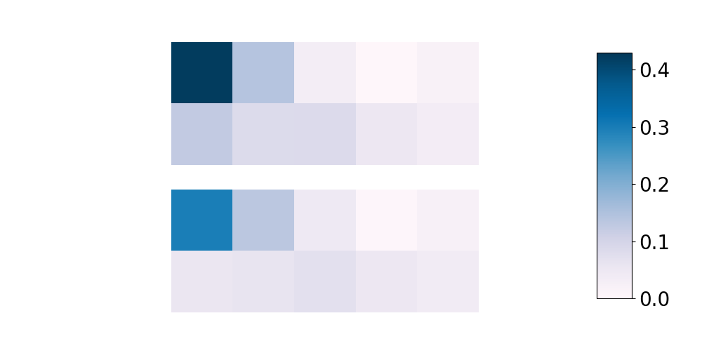
The terms involving the eigenvalues of in our bounds also support the intuition that adversarial robustness is a form of implicit regularization, which is visualized in Figure 1. In the one-dimensional linear classification setting, this phenomenon is well-understood (Tsipras et al., 2018; Dobriban et al., 2020), where robustness to adversarial perturbations prevent a robust feature vector from relying on an aggregate of small features. We note that in the case of state estimation, we have in general , and thus the quadratic factor in is in the lower bound (5).
3.2 Bounding for State Estimation
The adversarial risk does not admit a closed-form solution in general. Upper and lower bounds on the gap between the adversarial risk and standard risk, however, still highlight the role control theoretic quantities play in robustness-accuracy tradeoffs. We make the following simplifying assumption for presentation purposes going forward.
Assumption 3.1.
, , . We further assume that the system matrix , , is a scaled orthogonal matrix, such that controls the stability of the system.
As stated in 2.1, is always assumed to be observable. Generalizations of our subsequent results to generic dynamics and positive definite covariance matrices are stated and proven in Appendix C: although more notationally cumbersome, they nevertheless convey the same overall trends.
We first present a closed form for the standard risk which indicates the role that observability plays in robustness-accuracy tradeoffs.
Lemma 3.1.
The standard risk may be expressed as
Lemma 3.1 makes clear that the noise terms act as a regularizer: if , then and is achieved by . The gain of this filter has clear dependence upon the spectral properties of , indicating the key role that plays in the robustness-accuracy tradeoffs satisfied by an LTI system (1). We formalize this intuition next. As a first step, we specialize the lower bound in Theorem 3.1 to the dynamical system setting.
Lemma 3.2.
For any , the gap between and admits the following lower bound:
| (7) |
We now turn our attention to studying the tradeoffs enjoyed by the Kalman Filter/Smoother defined in Lemma 2.1. Since the Kalman estimator is the optimal estimator in the nominal setting and is commonly used in practice, instantiating Lemma 3.2 for captures the susceptibility of a nominal estimator to small adversarial perturbations. To simplify notation in the subsequent results, we will denote , and
| (8) |
With these definitions, we have the following theorem.
Theorem 3.2.
Suppose that is the Kalman estimator from Lemma 2.1. We have the following bound on the gap between and .
| (9) |
We see that the lower bound increases as the Frobenius norm of the observability gramian decreases. This indicates that as observability becomes uniformly low, i.e., if all eigenvalues of are small, then a nominal state estimator will have a large gap . Observe that increasing will increase the lower bound shown above when .
We now derive an upper bound on the gap between the standard and adversarial risk for any given . This bound follows from the upper bound in Theorem 3.1.
Lemma 3.3.
For any , the following bound holds
where is the symmetric square root of the covariance of .
Again, we consider how this upper bound looks for the Kalman estimator .
Theorem 3.3.
Suppose that is the Kalman state estimator from Lemma 2.1. Then
Furthermore, when , we have
The upper bound on the gap decreases as the minimum eigenvalue of the observability gramian increases. This indicates that as the observability of the system becomes uniformly large, the gap between standard and adversarial risk for the nominal Kalman estimator will decrease. Perhaps counter-intuitively, when observability is poor in some direction, i.e. when is small, increasing the sensor noise will actually decrease the above upper bound, as long as . This aligns with results demonstrating that injecting artificial noise can improve the robustness of state observers (Doyle and Stein, 1979), and is further consistent with our interpretation of noise as a regularizer following Lemma 3.1.
We note that since the properties of the observability gramian are tied to , it is not immediately clear how to extract the role of stability in either Equation 9 or Theorem 3.3. This is to be expected, as the fragility of the Kalman Filter has more to do with the observability of the system rather than its autonomous stability. For example, when , corresponding to maximal observability , and , then the dominant terms in the lower and upper bound are essentially independent of when is large.
4 Numerical Results
We now demonstrate that the theoretical results shown in the previous section predict the tradeoffs arising in Kalman Filtering problems.
Pareto Curves for Adversarial Kalman Filtering
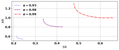
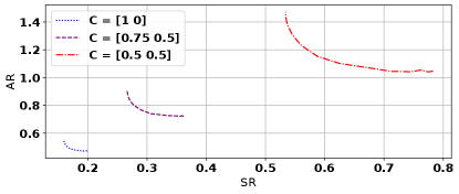
In this experiment we compute the Pareto-optimal frontier for adversarially robust Kalman filtering on systems with varying observability. We consider the system defined by the tuple where , and we vary . As approaches one the minimum eigenvalues of the observability gramian become small. In particular, for , , , the minimum eigenvalues of the observability gramian are given by and respectively. The adversarial budget is set to . Figure 2 shows the resulting tradeoff curves which demonstrate that as observability decreases, both and increase, as do the distance between the extremes of the Pareto curve. The results therefore support Section 3.2, where we showed shrinking the eigenvalues of increases the severity of the tradeoff between and .
Tradeoffs of Kalman Smoother versus Adversarially Robust Kalman Smoother
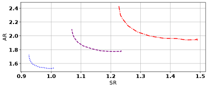
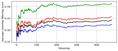
In Figure 3, we demonstrate the impact of adversaries on the risk incurred by an estimator optimized for versus . We consider initial state estimation of a system defined by the tuple , where we vary from to , such that the eigenvalues of increase as increases. The adversarial budget is fixed at . Evaluating the nominal and robust estimators on this class of systems, we see that the adversarially robust smoother has significantly smaller adversarial risk compared to the nominal Kalman smoother when observability is low. As observability increases, this advantage shrinks. This suggests that considering the tradeoffs from adversarially robust state estimation is most important when observability is low.
Tradeoffs with Nonlinear State Estimators
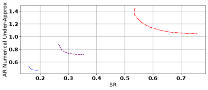
In Figure 4, we demonstrate empirically that the fundamental tradeoffs are not overcome by using nonlinear state estimators. In particular, we consider the system defined by , and as in the legend of the plots. We set the adversarial budget to . We solve for the Pareto boundary for the linear estimator as in Figure 2. We also consider a two layer network with ten neurons per layer and ReLU activation functions. To train this network, we perform an SGD procedure similar to that used in the linear case, with the exception being that we do not solve the exact adversary corresponding to each data point, but rather apply 100 steps of projected gradient ascent to find the adversarial perturbation. Once the neural network is trained, this same approach to find the adversary is used again to estimate the adversarial risk of the resultant estimator. As a result, the tradeoff curves shown for the neural network are an under-approximation to the true values of . As such, it appears that the neural network is getting roughly the same tradeoff curves as the linear estimator, which is expected due to the fact that linear estimators are optimal in the and settings (Zhou and Doyle, 1998).
Comparison with Kalman Filter, mixed , and Filters
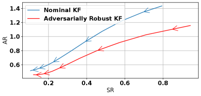
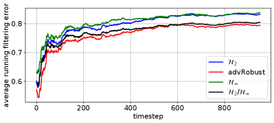
In Figure 5, we compare the performance of the adversarially robust Kalman filter with the optimal filter, a mixed filter which minimizes the norm subject to a norm bound of , and the nominal Kalman or filter. In particular, we consider the filtering problem for a trajectory generated by the system . For ease of computation, we use the stationary mixed, , and Kalman filters (Lewis et al., 2008; Caverly and Forbes, 2019), and the adversarially robust Kalman Filter for a horizon of 10 with adversarial budget . We consider a nominal setting, where process and state disturbances are Gaussian with covariances defined by and , and a setting to simulate sensor drift, where we have the white noise disturbances in addition to a sinusoidally varying measurement disturbance . The norm bound for the mixed filter was tuned to the value of for good performance on the sensor drift setting. As expected, the nominal Kalman filter performs best in the nominal setting with zero-mean disturbances. In the setting with sensor drift, however, the adversarially robust Kalman filter performs substantially better than the nominal and filters, and slightly better than the mixed controller. In both settings, the filter is overly conservative. Note that a key advantage of the adversarially robust controller is the interpretability of the robustness level determined by the parameter , which directly corresponds to the power of the adversarial disturbance. This feature is not shared by other filter designs, such as the norm bound in the mixed filter.
5 Conclusion
We analyzed the robustness-accuracy tradeoffs arising in Kalman Filtering. We did this in two parts. We first provided an algorithm to solve for the optimal adversarial perturbation, which can be used to trace out the Pareto boundary. We then bounded the gap between the adversarial and standard state estimation error in terms of the spectral properties of the observability gramian. These bounds extend upon the robustness-accuracy tradeoff results arising in the classification and linear regression settings. An interesting avenue of future work is to extend these results to infinite horizon filtering, and combine them with tradeoff analyses in LQR control (Lee et al., 2022) to provide an understanding of the adversarial tradeoffs in the control of partially observed linear systems. It would also be interesting to consider the adversarial tradeoffs of state estimation when adversarial state perturbations are also present.
Acknowledgements
Bruce Lee is supported by the Department of Defense through the National Defense Science & Engineering Graduate Fellowship Program. The research of Hamed Hassani is supported by NSF Grants 1837253, 1943064, 1934876, AFOSR Grant FA9550-20-1-0111, and DCIST-CRA. Nikolai Matni is funded by NSF awards CPS-2038873, CAREER award ECCS-2045834, and a Google Research Scholar award.
References
- Al Makdah et al. (2020) A. A. Al Makdah, V. Katewa, and F. Pasqualetti. Accuracy prevents robustness in perception-based control. In 2020 American Control Conference (ACC), pages 3940–3946. IEEE, 2020.
- Bottou et al. (2018) L. Bottou, F. E. Curtis, and J. Nocedal. Optimization methods for large-scale machine learning. SIAM Review, 60(2):223–311, 2018. doi: 10.1137/16M1080173.
- Boyd and Vandenberghe (2004) S. P. Boyd and L. Vandenberghe. Convex optimization. Cambridge university press, 2004.
- Carlini and Wagner (2016) N. Carlini and D. Wagner. Defensive distillation is not robust to adversarial examples. arXiv preprint arXiv:1607.04311, 2016.
- Carlini and Wagner (2017) N. Carlini and D. Wagner. Towards evaluating the robustness of neural networks. In 2017 IEEE symposium on security and privacy, pages 39–57. IEEE, 2017.
- Caverly and Forbes (2019) R. J. Caverly and J. R. Forbes. Lmi properties and applications in systems, stability, and control theory. arXiv preprint arXiv:1903.08599, 2019.
- Chen et al. (2020) L. Chen, Y. Min, M. Zhang, and A. Karbasi. More data can expand the generalization gap between adversarially robust and standard models. In International Conference on Machine Learning, pages 1670–1680. PMLR, 2020.
- Deka et al. (2020) S. A. Deka, D. M. Stipanović, and C. J. Tomlin. Dynamically computing adversarial perturbations for recurrent neural networks. arXiv preprint arXiv:2009.02874, 2020.
- Dobriban et al. (2020) E. Dobriban, H. Hassani, D. Hong, and A. Robey. Provable tradeoffs in adversarially robust classification. arXiv preprint arXiv:2006.05161, 2020.
- Doyle and Stein (1979) J. Doyle and G. Stein. Robustness with observers. IEEE Transactions on Automatic Control, 24(4):607–611, 1979. doi: 10.1109/TAC.1979.1102095.
- Goodfellow et al. (2014) I. J. Goodfellow, J. Shlens, and C. Szegedy. Explaining and harnessing adversarial examples. arXiv preprint arXiv:1412.6572, 2014.
- Hassibi et al. (1999) B. Hassibi, T. Kailath, and A. H. Sayed. Indefinite-quadratic estimation and control: a unified approach to H and H theories. SIAM studies in applied and numerical mathematics, 1999.
- Huang et al. (2017) S. Huang, N. Papernot, I. Goodfellow, Y. Duan, and P. Abbeel. Adversarial attacks on neural network policies. arXiv preprint arXiv:1702.02284, 2017.
- Javanmard et al. (2020) A. Javanmard, M. Soltanolkotabi, and H. Hassani. Precise tradeoffs in adversarial training for linear regression. In Conference on Learning Theory, pages 2034–2078. PMLR, 2020.
- Khargonekar et al. (1996) P. P. Khargonekar, M. A. Rotea, and E. Baeyens. Mixed H2/H filtering. International Journal of Robust and Nonlinear Control, 6(4):313–330, 1996.
- Lee et al. (2022) B. D. Lee, T. T. C. K. Zhang, H. Hassani, and N. Matni. Performance-robustness tradeoffs in adversarially robust linear-quadratic control, 2022.
- Lewis et al. (2008) F. L. Lewis, L. Xie, and D. Popa. Optimal and Robust Estimation: With an Introduction to Stochastic Control Theory. CRC Press, 2008.
- Lutter et al. (2021) M. Lutter, S. Mannor, J. Peters, D. Fox, and A. Garg. Robust value iteration for continuous control tasks. arXiv preprint arXiv:2105.12189, 2021.
- Madry et al. (2017) A. Madry, A. Makelov, L. Schmidt, D. Tsipras, and A. Vladu. Towards deep learning models resistant to adversarial attacks. arXiv preprint arXiv:1706.06083, 2017.
- Mandlekar et al. (2017) A. Mandlekar, Y. Zhu, A. Garg, L. Fei-Fei, and S. Savarese. Adversarially robust policy learning: Active construction of physically-plausible perturbations. In 2017 IEEE/RSJ International Conference on Intelligent Robots and Systems (IROS), pages 3932–3939. IEEE, 2017.
- Nakkiran (2019) P. Nakkiran. Adversarial robustness may be at odds with simplicity. arXiv preprint arXiv:1901.00532, 2019.
- Petersen et al. (2008) K. B. Petersen, M. S. Pedersen, et al. The matrix cookbook. Technical University of Denmark, 7(15):510, 2008.
- Pinto et al. (2017) L. Pinto, J. Davidson, R. Sukthankar, and A. Gupta. Robust adversarial reinforcement learning. In International Conference on Machine Learning, pages 2817–2826. PMLR, 2017.
- Raghunathan et al. (2019) A. Raghunathan, S. M. Xie, F. Yang, J. C. Duchi, and P. Liang. Adversarial training can hurt generalization. arXiv preprint arXiv:1906.06032, 2019.
- Szegedy et al. (2013) C. Szegedy, W. Zaremba, I. Sutskever, J. Bruna, D. Erhan, I. Goodfellow, and R. Fergus. Intriguing properties of neural networks. arXiv preprint arXiv:1312.6199, 2013.
- Tsipras et al. (2018) D. Tsipras, S. Santurkar, L. Engstrom, A. Turner, and A. Madry. Robustness may be at odds with accuracy. arXiv preprint arXiv:1805.12152, 2018.
- Xie et al. (2020) C. Xie, M. Tan, B. Gong, A. Yuille, and Q. V. Le. Smooth adversarial training. arXiv preprint arXiv:2006.14536, 2020.
- Zhang et al. (2019) H. Zhang, Y. Yu, J. Jiao, E. P. Xing, L. E. Ghaoui, and M. I. Jordan. Theoretically principled trade-off between robustness and accuracy. arXiv preprint arXiv:1901.08573, 2019.
- Zhou and Doyle (1998) K. Zhou and J. C. Doyle. Essentials of Robust Control. Prentice-Hall, 1998.
Appendix A Kalman Filtering State Space Solution
Consider the setting defined in Section 2.1, i.e. we have a dynamical system which progresses according to
with , , . Consider estimating state given measurements . The minimum mean square estimator is given by
This can be written as an integral
where denotes the conditional density of given the measurements. The objective is convex in , and thus we can find the minimizer by setting the gradient with respect to to zero. In particular, we have
where dominated convergence theorem permits the exchange of integration and differentiation. Therefore, the state estimate may be expressed
Thus we can determine the state estimates as the mean of the conditional distribution . This may be computed recursively. In particular, let be the random variable with probability density function . Then for all , we have that where
| (10) | ||||
To see that this is the case, recall that , by assumption. Now suppose that . Observe that
Thus
Now, given , observe that .
Appendix B Proofs from Section 2
B.1 Proof of Lemma 2.1
B.2 Proof of Correctness for Algorithm 1
Recalling the optimization problem
| (P) | ||||
and the corresponding KKT conditions:
The third condition implies that . We assume , otherwise the problem is trivial. Then using the SVD of to re-arrange the first stationarity condition, we get
Maximizing a convex function over a convex set achieves its maximum on the boundary; it suffices to search over . We now consider two cases: and .
-
•
In the first case , we know must be invertible, and thus
where are the columns of . By 2.1, we know . Observe that
is a strictly monotonically decreasing function when , and converges to when . This implies there is a unique such that , which can be numerically solved for in various ways, such as bisection. Such methods can be initialized by setting the left boundary to , corresponding to , and the right boundary to a precomputable over-estimate such that . As an example, one such crude over-estimate can be derived by observing
Hölder’s inequality Therefore, bisection can solve for up to a desired tolerance in at most iterations, which is linear bit-complexity over problem parameters. Since enjoys favorable regularity properties such as monotonicity, strict convexity, and smoothness on an open interval around , more advanced root-finding methods such as variants of Newton’s method or the secant method can be employed for superlinear convergence.
-
•
Now we consider the case where . In this case, will no longer be unique, and will come in the form
where † denotes the Moore-Penrose pseudoinverse, and is any unit vector lying in the null-space of , which is precisely characterized in this case by
with denoting the th column of . To find the appropriate scaling , we observe
Combining our precise characterization of using the columns of , and the formula for , we can extract an optimal perturbation vector . Therefore, we have demonstrated that (P), as well as extracting its optimal solution, can be solved to arbitrary precision.
Appendix C General Statements and Proofs for Section 3
C.1 Proof of Theorem 3.1
Theorem 3.1 Given any , we have the following lower bound on :
and a corresponding upper bound
where and are the minimum and maximum eigenvalues of , respectively.
Proof: First recall the definitions of SR and AR:
Given fixed , let us define the quantity . Writing out the inner maximization of AR we have:
Observe that this is equivalent to the problem
| (P1) | ||||
We now recall the S-lemma for quadratic functions.
Lemma C.1 (S-lemma).
Given quadratic functions , suppose there exists such that . Then,
if and only if
Using this lemma, we set , . We observe that trivially, there exists such that . Now given feasible for (P1), we observe that by our constraints, any such that immediately implies . By the S-lemma, this is equivalent to the existence of some such that
for all . Therefore, we can re-write the optimization problem (P1) into
| (P2) | ||||
Re-arranging the terms in the quadratic expression, we get:
Now we recall a property of Schur complements.
Lemma C.2 (Schur Complement).
Given , we have
Applying this to (P2), we see the constraints can be re-written
Therefore, we get the optimization problem
However, this is clearly equivalent and has the same optimal value as the following problem
Notice that so far we are simply considering equivalent formulations to the original optimization. The ensuing step is where the lower and upper bounds (5) and arise. Recall the Neumann series, where since , we have
From the Neumann series, we see that we can upper and lower bound the inverse using geometric series of the largest and smallest eigenvalues of , respectively,
From now on, we will deal with the inverse, since instead of the pseudo-inverse we can take the infimum of the above problem, which is bounded from below. Let us consider the lower bound first. The upper bound follows using the exact same analysis. We have
Therefore, we have
We now make a second relaxation:
which we get by deriving the unconstrained minimizer . Now putting expectations on both sides of the inequality, we get
In the subsequent full statements of the corresponding results in the paper, we do not make 3.1, and instead consider general observable , where , and positive definite noise covariances .
C.2 General Statement of Lemma 3.1
Lemma 3.1. The standard risk may be expressed as
Proof: This follows simply by expanding the norm inside the expectation, and noticing that since , , are defined to be zero-mean Gaussian random vectors, their cross terms vanish. More precisely, we have
C.3 General Statement of Lemma 3.2
Proof: Applying the lower bound (5), we have
Then to derive the lower bound (C.3), we observe that the random vector
is a zero-mean Gaussian with covariance
We can also write where . Consider the diagonalization of . Then
where is the th row of and is the th singular value of . We have that
We have by equivalence of norms, . Therefore,
and thus
where . The quantity is the expected value of a folded standard normal, which is , while . Putting this together, we have that
From the above bound, we may now derive a cruder lower bound from which we can observe a dependence on the singular values of the observability grammian, . In particular, begin with the expression above, and note that the terms involving and are positive definite to achieve a lower bound in terms of :
which completes the proof of inequality (C.3).
Introducing additional notation to express the Kalman estimator will be helpful in subsequent sections. Let
| (12) | ||||
where is a block downshift operator, with blocks of size . With this notation, the Kalman estimator given in Lemma 2.1 may be rewritten more compactly as
C.4 General Statement of Theorem 9
Theorem 9. Suppose that is the Kalman estimator from Lemma 2.1. Then we have the following bound on the gap between and .
Proof: We begin by writing the Kalman estimator using the notation defined in (12)
Suppose the rank of is . Then the singular value decomposition of can be taken to be
where with , while and . We can now lower bound the Frobenius norm of as follows.
Note that . Therefore
| (13) | ||||
Now observe that
| (14) |
Also note that . We have that
Then
| (15) |
C.5 Proof of Lemma 3.3
Lemma 3.3. For any , the following bound holds
where is the symmetric square root of the covariance of .
Proof: By Theorem 3.1,
We can upper bound by bounding the expectation of the euclidean norm of a normal random variable. In particular, let be a dimensional standard normal random variable, so that , where is defined as the covariance of , and is its symmetric square root. Let be the eigenvalue decomposition of so that
Now define . We have that . Then the above quantity equals . Jensen’s inequality tells us that
from which the theorem follows.
C.6 General Statement of Theorem 3.3
Theorem 3.3. Suppose that is the Kalman state estimator given by Lemma 2.1. Then the gap between and is upper bounded by
Furthermore, if , and defining , we get the bound
Proof: By Lemma 3.3, upper bounding the gap between and reduces to upper bounding and . First consider . Equivalence of norms tells us that
| (16) |
Recalling the notation defined in (12), the Kalman filter may be expressed as . We may also express in terms of this notation: . To upper bound the spectral radius of this, we can leverage triangle inequality and submultiplicativity
Note that . Then by submultiplicativity,
We can further upper bound in terms of system properties. In particular, we have
Thus
| (17) |
Next we obtain a bound on . As in the proof of Theorem 9, we will assign and take the singular value decomposition of to be where with , while and .
A simple bound on the last maximization would be
| (18) |
Note that , so . Then
| (19) |
Then the first half of the theorem follows by combining the result of Lemma 3.3 with (16), (17) and (19).
However, if , then the maximum (18) is attained at
Therefore, when , we have the more precise bound
which leads to the second half of the theorem.