Age of Computing: A Metric of Computation Freshness in Communication and Computation Cooperative Networks
Abstract
In communication and computation cooperative networks (3CNs), timely computation is crucial but not always guaranteed. There is a strong demand for a computational task to be completed within a given deadline. The time taken involves both processing time, transmission time, and the impact of the deadline. However, a measure of such timeliness in 3CNs is lacking. To address this gap, we propose the novel concept of Age of Computing (AoC) to quantify computation freshness in 3CNs. Built on task timestamps, AoC is universally applicable metric for dynamic and complex real-world 3CNs. We evaluate AoC under two types of deadlines: (i) soft deadline, tasks can be fed back to the source if delayed beyond the deadline, but with additional latency; (ii) hard deadline, tasks delayed beyond the deadline are discarded. We investigate AoC in two distinct networks. In point-to-point, time-continuous networks, tasks are processed sequentially using a first-come, first-served discipline. We derive a general expression for the time-average AoC under both deadlines. Utilizing this expression, we obtain a closed-form solution for M/M/1 - M/M/1 systems under soft deadlines and propose an accurate approximation for hard deadline. These results are further extended to G/G/1-G/G/1 systems. Additionally, we introduce the concept of computation throughput, derive its general expression and an approximation, and explore the trade-off between freshness and throughput. In the multi-source, time-discrete networks, tasks are scheduled for offloading to a computational node. For this scenario, we develop AoC-based Max-Weight policies for real-time scheduling under both deadlines, leveraging a Lyapunov function to minimize its drift.
Index Terms — Age of computing, computation freshness, communication and computing cooperated networks, time-average AoC, Max-Weight Policy.
I Introduction
In the 6G era, emerging applications such as the Internet of Things (IoT), smart cities, and cyber-physical systems have significant demands for communication and computation cooperative networks (3CNs), which provide faster data processing, efficient resource utilization, and enhanced security [1]. 3CNs originated from mobile edge computing (MEC) technology, which aims to complete computation-intensive and latency-critical tasks, with the paradigm deploying distributedly tons of billions of edge devices at the network edges [2]. Besides MEC, 3CNs include fog computing and computing power networks. Fog computing can be regarded as a generalization of MEC, where the definition of edge devices is broader than that in MEC [3]. Computing power networks refers to a broader concept of distributed computing networks, including edge, fog, and cloud computing [4]. In all 3CNs, there is no established metric for capturing the freshness of computation. Recently, a notable metric called the Age of Information (AoI) has been proposed to describe information freshness in communication networks [5]. The AoI metric has broad applications in various communication and control contexts, including random access protocols [6], multiaccess protocols [7], remote estimation [8], wireless-powered relay-aided communication networks [9], and network coding [10, 11].
However, applying AoI in 3CNs is inappropriate because it only addresses communication latency and does not account for computation latency. In this paper, we propose a novel metric called the age of computing (AoC) to capture computation freshness in 3CNs. A primary requirement in 3CNs is that computational tasks are processed as promptly as possible and within a maximum acceptable deadline. The core idea of AoC is to combine communication delay, computation delay, and the impact of the maximum acceptable deadline. Communication and computation delays are caused by the transmission and processing of computational tasks, while the impact of the maximum acceptable deadline accounts for additional delays when task delays exceed the users’ acceptable threshold.
I-A Related Work
All related papers can be divided into two broad categories. The first category investigates information freshness in edge and fog computing networks. The second category focuses on freshness-oriented metrics.
I-A1 Information Freshness in Edge/Fog Computing Networks
In edge and fog computing networks, tasks or messages typically go through two phases: the transmission phase and the processing phase. The basic mathematical model for these networks is established as two-hop networks and tandem queues.
The first study to focus on AoI for edge computing applications is [12], which primarily calculated the average AoI. As an early work, [13] established an analytical framework for the peak age of information (PAoI), modeling the computing and transmission process as a tandem queue. The authors derived closed-form expressions and proposed a derivative-free algorithm to minimize the maximum PAoI in networks with multiple sensors and a single destination. Subsequently, [14] modeled the communication and computation delays as a generic tandem of two first-come, first-serve queues, and analytically derived closed-form expressions for PAoI in M/M/1-M/D/1 and M/M/1-M/M/1 tandems. Building on [14], [15] went further by considering both average and peak AoI in general tandems with packet management. The packet management included two forms: no data buffer, and a one-unit data buffer with last-come first-serve displine. This work illustrated how computation and transmission times could be traded off to optimize AoI, revealing a tradeoff between average AoI and average peak AoI. Expanding on [15], [16] explored the information freshness of Gauss-Markov processes, defined as the process-related timeliness of information. The authors derived closed-form expressions for information timeliness at both the edge and fog tiers. These analytical formulas explicitly characterize the dependency among task generation, transmission, and execution, serving as objective functions for system optimization. In [17], a multi-user MEC network where a base station (BS) transmits packets to user equipment was investigated. The study derived the average AoI for two computing schemes—local computing and edge computing—under a first-come, first-serve discipline.
There are other relevant works such as [18, 19, 20, 21]. [18] investigated information freshness in MEC networks from a multi-access perspective, where multiple devices use NOMA to offload their computing tasks to an access point integrated with an MEC server. Leveraging tools from queuing theory, the authors proposed an iterative algorithm to obtain the closed-form solution for AoI. In [19], a F-RAN with multiple senders, multiple relay nodes, and multiple receivers was considered. The authors analyzed the AoI performances and proposed optimal oblivious and non-oblivious policies to minimize the time-average AoI. [20] and [21] explored AoI performances in MEC networks using different mathematical tools. [20] considered MEC-enabled IoT networks with multiple source-destination pairs and heterogeneous edge servers. Using game-theoretical analysis, they proposed an age-optimal computation-intensive update scheduling strategy based on Nash equilibrium. Reinforcement learning is also a powerful tool in this context. [21] proposed a computation offloading method based on a directed acyclic graph task model, which models task dependencies. The algorithm combined the advantages of deep Q-network, double deep Q-network, and dueling deep Q-network algorithms to optimize AoI.
I-A2 Freshness-oriented Metrics
The AoI metric, introduced in [5], measures the freshness of information at the receiver side. AoI depends on both the frequency of packet transmissions and the delay experienced by packets in the communication network [6]. When the communication rate is low, the receiver’s AoI increases, indicating stale information due to infrequent packet transmissions. However, even with frequent transmissions, if the system design imposes significant delays, the receiver’s information will still be stale. Following the introduction of AoI, several related metrics were proposed to capture network freshness from different perspectives. Peak AoI, introduced in [7], represents the worst-case AoI. It is defined as the maximum time elapsed since the preceding piece of information was generated, offering a simpler and more mathematically tractable formulation.
Nearly simultaneously, the age of synchronization (AoS) [22] and the effective age [23] were proposed. AoS, as a complementary metric to AoI, drops to zero when the transmitter has no packets to send and grows linearly with time until a new packet is generated [22]. The effective age metrics in [23] include sampling age, tracking the age of samples relative to ideal sampling times, and cumulative marginal error, tracking the total error from the reception of the latest sample to the current time.
Later, the age of incorrect information (AoII) [24] and the urgency of information (UoI) [25] were introduced. AoII addresses the shortcomings of both AoI and conventional error penalty functions by extending the concept of fresh updates to “informative” updates—those that bring new and correct information to the monitor side [24]. UoI, a context-based metric, evaluates the timeliness of status updates by incorporating time-varying context information and dynamic status evolution [25], which enables analysis of context-based adaptive status update schemes and more effective remote monitoring and control.
Despite the variety of freshness-oriented metrics proposed, none are applicable for capturing computation freshness in 3CNs. None of these metrics simultaneously address the impact of both communication and computation delays, as well as the maximum acceptable deadline. Motivated by the need for a metric capturing freshness in 3CNs, we propose the AoC metric in this paper.
I-B Contributions
This paper introduces the Age of Computing (AoC), a novel metric designed to capture computation freshness in 3CNs (see Definition 3). The AoC concept is built on tasks’ arrival and completion timestamps, which makes it applicable to dynamic and complex real-world 3CNs. The AoC is defined under two types of deadlines: (i) soft deadline, i.e., if the task’s delay exceeds the deadline, the outcome is still usable but incurs additional latency; (ii) hard deadline, i.e., if the task’s delay exceeds the deadline, the outcome is discarded, and the task is considered invalid.
We then theoretically analyze the time-average AoC under both types of deadlines in a linear topology comprising a source, a transmitter, a receiver, and a computational node. Tasks arrive at the source at a constant rate and immediately enter a communication queue at the transmitter. After being transmitted/offloaded to the receiver, tasks are forwarded to the computational node for processing in a computation queue. The queuing discipline considered is first-come, first-served.
Under the soft deadline, we first derive a general expression for the average AoC (see Theorem 1). We then study a fundamental scenario where the task arrival process follows a Poisson distribution, and the transmission and computation delays adhere to exponential distributions—forming an M/M/1-M/M/1 system. In this case, we derive a closed-form expression for the average AoC (see Theorem 2). Subsequently, we extend our analysis to a more general scenario where the task arrival process follows a general distribution, and the transmission and computation delays also follow general distributions—resulting in a G/G/1-G/G/1 system. For this case, we derive the expression for the average AoC as well (see Theorem 3).
Under the hard deadline, we first derive a general expression for the average AoC (see Theorem 4). This expression involves intricate correlations, making it highly challenging to obtain a closed-form solution, even for an M/M/1-M/M/1 system. To address this, we provide an approximation of the average AoC and demonstrate its accuracy when the communication and computation rates are significantly larger than the task generation rate (see Theorem 5). We also define computation throughput as the number of tasks successfully fed back to the source per time slot (see Definition 4). A general expression for computation throughput is derived (see Lemma 1), along with an approximation (see Proposition 1). Furthermore, we explore the trade-off between computation freshness and computation throughput (see Lemma 2). In the end, we extend the accurate approximations for both the average AoC and computation throughput to more generalized scenario involving G/G/1-G/G/1 systems (see Theorem 6 and Proposition 2).
Finally, we apply the AoC concept to develop optimal real-time scheduling strategies focused on enhancing computation freshness in multi-source networks. Recognizing the importance of recent computational tasks, we adopt a preemptive scheduling rule. For real-time scenarios, we propose AoC-based Max-Weight policies for both deadlines (see Algorithms 1 and 2). By constructing a Lyapunov function (see (28)) and its drift (see (29)), we show that these policies minimize the Lyapunov drift in each time slot (see Propositions 3 and 4).
The remaining parts of this paper are organized as follows. Section II proposes and discusses the novel concept AoC. Section III and Section IV derive theoretical results for the AoC under the soft and hard deadlines, respectively. Section V designs real-time AoC-based schedulings in multi-source networks are proposed. We numerically verify our theoretical results in Section VI and conclude this work in Section VII.
II Age of Computing
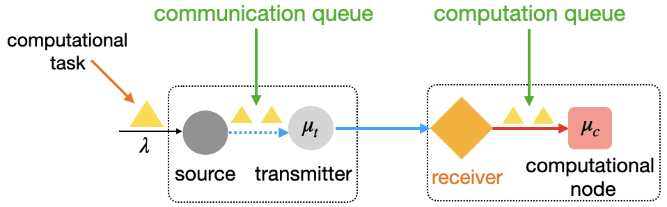
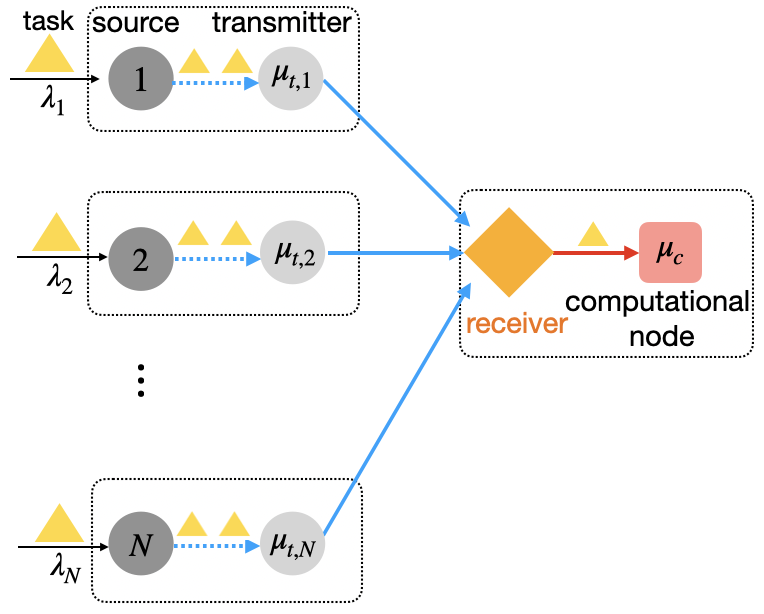
In this section, we introduce the mathematical formulation of the novel concept, Age of Computing (AoC), which quantifies the freshness of computations within 3CNs. Consider a line topology comprising a source, a transmitter, a receiver, and a computational node (sink), as depicted in Fig. 1. In this topology, both the receiver and the computational node are equipped with caching capabilities. The process begins with the source generating/offloading computational tasks, which are immediately available at the transmitter and enter a communication queue awaiting transmission. Once transmitted, the tasks are received and cached by the receiver, where they await processing. Afterward, tasks are handed off to the computational node (sink), where they are processed and eventually depart from the system.
II-A Definition
In the network, the queuing despline follows a first-come first-serve approach. For any task , let denote the arrival time at the source, the time when the computation starts at the computational node, and the time when the computation completes. The delay of task is then defined as . A task is considered valid if its outcome can be fed back to the source111The feedback is an acknowledgment message with a small bit size, commonly used in communication systems to confirm the successful receipt of data.; otherwise, it is deemed invalid.
Definition 1.
(informative, processing, and latest tasks). The index of the informative task during , denoted by , is given by
| (1) |
The index of the processing task during , denoted by , is given by
| (2) |
The index of the latest task during , denoted by , is given by
| (3) |
Based on Definition 1, an informative task is a valid task that brings the latest information. The processing is the current task being processed, and the latest refers to the last completed task. The informative task and the latest task are not necessarily the same, i.e., . They coincide () only when the latest task is also informative. At any time , if the computational node is idle (no task is being processed), then the processing task is exactly the latest one, i.e, . If the computational node is occupied (a task is being processed), then . In summary, we have .
Definition 2.
A maximum acceptable deadline can be categorized into two types:
-
•
Soft deadline: A task is considered valid if its delay .
-
•
Hard deadline: A task is considered invalid if its delay .
We define the index of lastest task within whose delay does not exceed the threshold as:
| (4) |
Under the soft deadline, we have , while under the hard deadline, we have . The computation freshness at the computational node is formally defined as follows.
Definition 3.
(AoC). Under the soft deadline, the age of computing (AoC) is defined as the random process
| (5) |
Under the hard deadline, the AoC is defined as the random process
| (6) |
The key distinction in Definition 3 lies in how computation freshness is assessed under hard and soft deadlines:
-
•
Under the hard deadline, computation freshness in (6) is determined solely by the informative tasks, as tasks with delays exceeding the threshold are deemed invalid.
-
•
Under the soft deadline, computation freshness in (3) accounts for both the informative tasks (i.e, ) and an additional latency incurred if the task being processed experiences a significant instantaneous delay (i.e, ). In particular, the additional latency includes components:
-
–
The indicator function denotes whether a task is being processed at the computational node.
-
–
The ratio represents the frequency of task delays exceeding the deadline up to time , effectively quantifying the level/frequency of conflict with respect to the deadline (up to time ).
-
–
The term quantifies the amount by which the delay of the task currently being processed exceeds the threshold.
-
–
This additional latency, calculated by the computational node, vanishes as soon as the current task is completed.
-
–
The concept of information freshness, known as AoI [5], reflects the cumulative delay over a given time period. Building on this foundation, AoC extends the notion to computational tasks, representing the cumulative delay associated with their processing. AoC provides a more comprehensive understanding of the timeliness of computations in a system. While related, AoC and AoI are fundamentally distinct in their definitions and physical interpretations: AoC evaluates the freshness of the informative task (may including an additional latency incurred by the task being processed), whereas AoI focuses on the freshness of the latest task.
Since the AoC with , captures the computation freshness at time , we often consider the time-average AoC over a period to measure the computation freshness of a network. As , we define the average AoC of a network as
| (7) |
Finally, we summarize the important notations and their descriptions in the paper in Table I.
| the index of computational tasks | |
|---|---|
| the threshold | |
| the arrival time of task at the source | |
| time when the computation completes | |
| the time when the computation completes | |
| the index of the informative task during | |
| the index of the processing task during | |
| the index of the latest task during | |
| the index of the latest task with a delay during | |
| the AoC under the soft deadline in time | |
| the AoC under the hard deadline in time | |
| the time-average AoC the soft deadline | |
| the time-average AoC the hard deadline | |
| the communication rate | |
| the computation rate | |
| the inter-arrival time between task and task | |
| the delay of task | |
| the number of invalid tasks between two valid tasks |
II-B Insights and Applications
From (3) and (6), we observe that the only notation used is the timestamp, specifically the arrival timestamp and the departure timestamp . To establish this concept, we intentionally avoid incorporating physical parameters such as bandwidth, GPU cycles, or caching. Instead, we focus solely on the use of timestamps. The reason for this choice is that the timestamp is the most fundamental and universally applicable metric that can be recorded by the destination (i.e., computational nodes) in any realistic 3CNs.
Let denote the timestamp when task reaches the receiver. The difference represents the transmission delay for task , which is determined by the communication capability. This delay can be influenced by various network characteristics, such as bandwidth, information size, signal-to-noise ratio, channel capacity, network load, transmission protocols, and more. On the other hand, the difference represents the computation delay for task , which depends on the computation capability. This delay is influenced by factors such as GPU cycles, task complexity, node load, memory size, access speed, I/O scheduling, and more. Finally, the total delay of task , given by , encompasses both the transmission and computation delays. As such, it is influenced by both the communication and computation capabilities. The AoC concept effectively captures the impact of both these factors on task performance.
The AoC concept is also applicable in dynamic and complex environments, such as mobile computing. In such settings, the communication network may experience interruptions or temporary failures due to factors like signal loss, interference, or mobility-related issues (e.g., moving out of network coverage). Tasks may experience temporary delays in a queue due to these disruptions. Nevertheless, the AoC concept remains applicable. To calculate the AoC, we only need the timestamps of tasks (i.e., ). As long as timestamps can be recorded, the AoC can be calculated, regardless of disruptions.
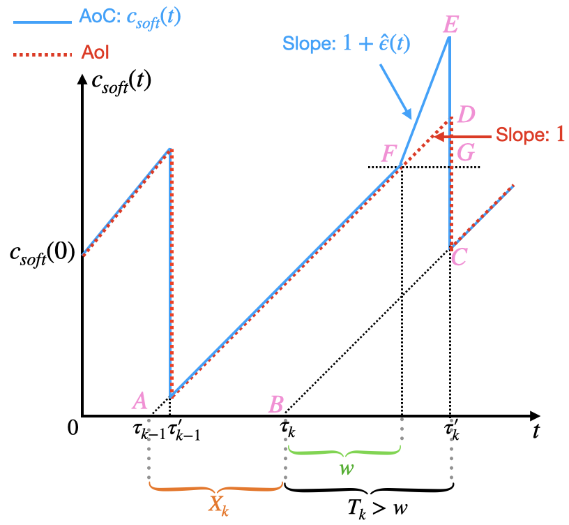
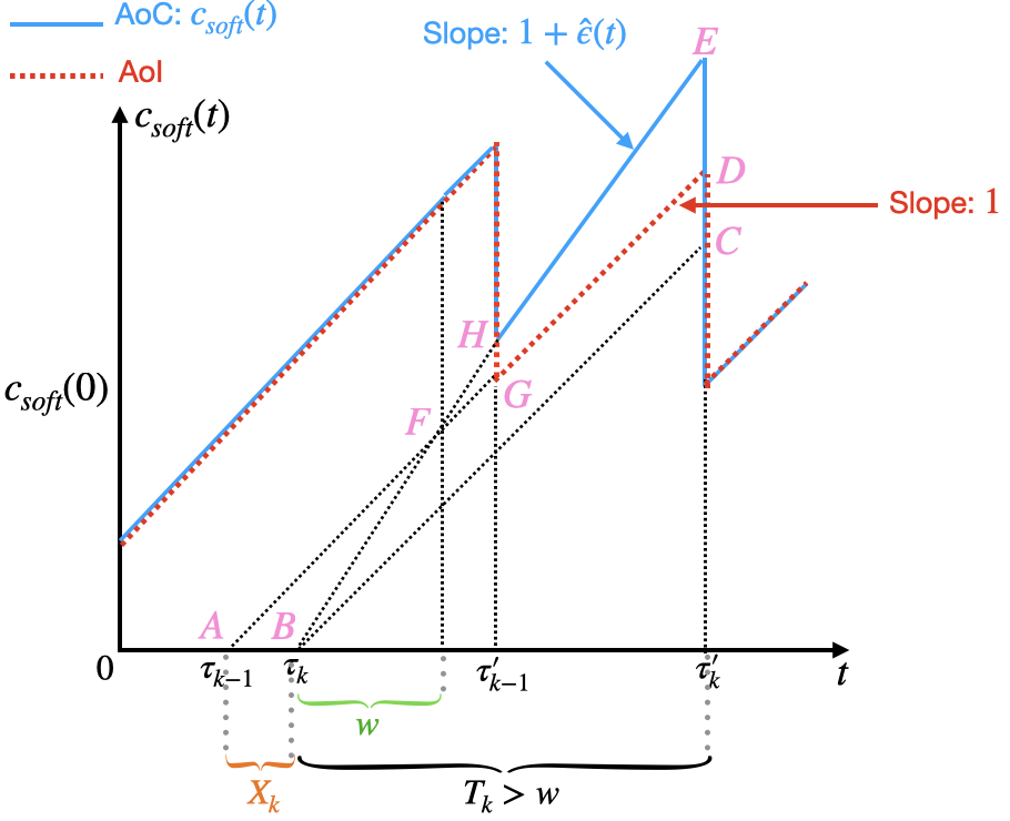
III AoC Analysis under the Soft Deadline
In this section, we first provide graphical insights into the curve of the AoC (see Fig. 2). Next, we derive a general expression for the time-average AoC, presented in Theorem 1 (Section III-A). Following this, we analyze the expression in a fundamental case: the M/M/1 - M/M/1 tandem system, as detailed in Theorem 2 (Section III-B). Finally, we extend the average AoC expression to more general cases, specifically G/G/1 - G/G/1 tandem systems, as discussed in Theorem 3 (Section III-C).
III-A General Expression for
For analytical tractability, we consider a simplified model: (i) A task is represented by , where denotes the task’s input data size, represents the maximum acceptable deadline, and indicates the computation workload [1]. (ii) The network is characterized by , where is the data rate of the communication channel at the transmitter, and is the CPU cycle frequency at the computational node. (iii) The expected transmission delay of a task is , and the expected computation delay is . (iv) Both delays each follow their respective distributions. We define and as the communication rate and computation rate, respectively.
Let and . From [5], the AoI concept shares the same formula as . Using the AoI curve as a benchmark, the AoC curve is depicted in Fig. 2. In Fig. 2 (a), the delay of task exceeds the threshold (), but any waiting time before task is processed does not surpass the threshold. When the (instantenous) delay of a task is less than the deadline , the AoC curve coincides with the AoI curve. However, when the (instantenous) delay of a task exceeds the deadline , the portion of the delay exceeding the deadline increases at a rate . In Fig. 2 (b), both the delay of task and the waiting time bofore task is processed () exceed the threshold. When the processing of task begins, an additional latency is introduced. As a result, at time , there is an upwardjump (additional latency) of . Subsequently, the AoC curve increases at a rate .
To uncover theoretical insights into the average AoC, we investigate it within queue-theoretic systems. We assume a stationary queuing discipline with a first-come, first-serve approach. On the source side, computational tasks arrive according to a stationary stochastic process characterized by a constant average rate. The inter-arrival between consecutive tasks is denoted by . Upon arrival, each task experiences a transmission delay, denoted by , at the transmitter, which follows a distribution with a constant expectation. Similarly, the computation delay denoted by , at the computational node also follows a distribution with a constant expectation. Let the delay of task be denoted by . In queuing systems, this delay is referred to as the system time, and we use these terms interchangeably. Under the stationary queuing discipline, , , , and are i.i.d, respectively.
Theorem 1.
The average AoC can be calculated as
| (8) |
where .
Proof.
The proof is given in Appendix A. ∎
III-B Average AoC in M/M/1-M/M/1 Systems
In this section, we let the inter-arrival follows an exponential distribution with parameter , meaning that computational tasks arrive at the source according to a Poisson process characterized by an average rate of . Let and have exponential distributions with parameters () and (), respectively. In other words, the network forms an M/M/1-M/M/1 tandem.
Theorem 2.
Let and . Denote
The closed form expression for is given by: if , then
| (9) |
if , then
| (10) |
III-C Extension: Average AoC in G/G/1-G/G/1 Systems
In this section, we let the inter-arrival follows a general distribution with , meaning that computational tasks arrive at the source according to a general stochastic process characterized by an average rate of . Let and have general distributions with and , respectively. In other words, the network forms an G/G/1-G/G/1 tandem.
To obtain the average AoC, it is necessary to know the stachastic information about the inter-arrival interval, the service delay at the transmission and computation nodes, and the system time of a task in both the transmission and computation queues. Let the system times of a task in the transmission and computation queues be denoted as and , respectively.
Note that sequences , , , and are i.i.d with respect to , respectively. The correpsonding density functions are denoted by , , , , and , respectively. The joint density function of and is denoted as . The following assumptions are then required.
Assumption 1.
The density functions , , , and are known.
Based on Assumption 1, the following steps can be taken:
-
•
By integrating , we can obtain the marginal density functions and .
-
•
Since (respectively, ) is independent of (respectively, ), and the marginal density functions and are avaibale, we can derive the density functions of the waiting times in both queues, namely and , through inverse convolution.
-
•
Given that , , and are known, we can again apply inverse convolution to derive the joint density functions and .
Theorem 3.
Proof.
The proof is given in Appendix C. ∎
Remark 1.
Remark 2.
Assumption 1 provides the minimum sufficient conditions for the closed form of the average AoC. However, it does not guarantee the convergence of , which heavily depends on the distributions of , , , , and .
IV AoC under the Hard Deadline
In this section, we first provide graphical insights into the curve of the AoC (see Fig. 3). Next, we derive a general expression for the time-average AoC, presented in Theorem 4 (Section IV-A). Following this, we accurately approximate the expression in a fundamental case: the M/M/1-M/M/1 system, as detailed in Theorem 5 (Section IV-B). In addition, we define computation throughput (see Definition 4 in Section IV-C) and derive its expression (see Lemma 1 in Section IV-C). Subsequently, we investigate the trade-off between computation freshness and computation throughput (see Lemma 2 in Section IV-C). Finally, we generalize the accurate approximations for both the average AoC and computation throughput to broader cases, specifically G/G/1-G/G/1 systems, as presented in Theorem 6 and Proposition 2 (Section IV-D).
IV-A General Expression for
From (6) in Definition 3, under the hard deadline, is solely determined by informative tasks. When , all tasks are considered invalid, leading to , which increases linearly with time . Conversely, when , there is no dedline, and all tasks are considered valid. In this case for all , so , which is only affected by the lastest task.
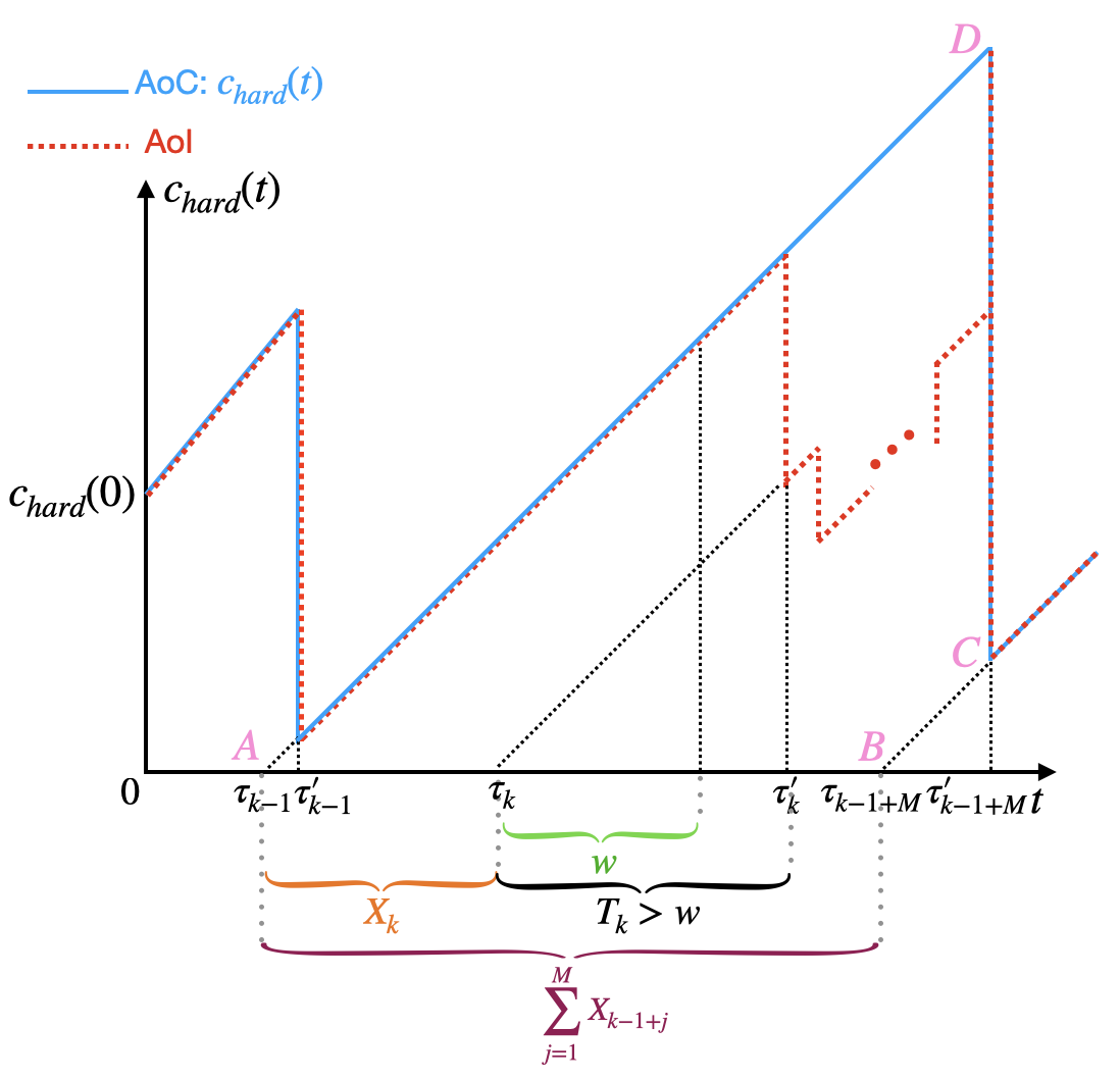
The AoC curve is depicted in Fig. 3, with the curve of AoI (see [5]) as a benchmark. In this figure, task is valid, so both AoI and AoC decreases at time . Suppose that after task , the next valid task has the index . Here, is a random varibale with the distribution
| (12) |
From (IV-A), . Since the network is stationary, the random variable associated with every valid task has the identical distribution as in (IV-A). The AoC does not decrease at times , , , , and decreases at time . In the interval , the AoC increases linearly with time .
Theorem 4.
The average AoC can be calculated as
| (13) |
Proof.
The proof is given in Appendix D. ∎
Although the general expression for the average AoC is given by (13), a further exploration on this expression is challenging due to a couple of correlations involved. These correlations are detailed as follows.
-
(i)
Correlation between delays: In the queuing system, if the delay of task , , increases, the waiting time for task also increases, leading to a larger delay for task , . Hence, the sequence consists of identical but positively correlated delays.
-
(ii)
Correlation between delays and (defined in (IV-A)): According to (IV-A), is the first index such that while all previous . A higher value of suggests a higher likelihood of subsequent values (for ) also being high, thus making larger because it takes longer for a to be less than or equal to . This indicates that are are positively correlated.
-
(iii)
Correlation between the inter-arrival times and delays : If is larger, meaning that the inter-arrival time between task and task is longer, then is likely smaller because the waiting time for task is reduced. Therefore, and are negatively correlated.
-
(iv)
Correlation between the inter-arrival times and : Since are are negatively correlated, and and are positively correlated, and are negatively correlated.
IV-B Average AoC in M/M/1-M/M/1 Systems
Due to all these correlations, it is extremely challenging to derive the closed-form expression for in (13). However, we can approximate it accurately under specific conditions.
Theorem 5.
Remark 3.
By exchanging and in (5) and (5), we observe that remains unchanged. This indicates that is symmetric with respect to . From a mathematical standpoint, this symmetry implies that both communication latency and computation latency equally affect . Therefore, in practical terms, to improve the computation freshness , one can reduce either the communication latency or the computation latency, as both have the same impact on the overall freshness.
IV-C Computation Throughput
Unlike the hard deadline, the frequency of informative tasks is influenced by two facts: the arrival rate and the deadline . We define the frequency of informative tasks as computation throughput. Formally, we have the following definition.
Definition 4.
(Computation Throughput) The computation throughput is defined as
| (17) |
Lemma 1.
The computation throughput is given by,
| (18) |
In (18), the arrival rate is reflected in , while the deadline is captured by . It is worth noting that Definition 4 can apply to the case with a soft deadline. Under the soft deadline, (17) implies that , which is a trivial case. Therefore, we did not investigate the computation throughput concept in Section III.
Proposition 1.
Remark 4.
(Upper Bound) According to (IV-A), a higher value of suggests a higher likelihood of subsequent values (for ) also being high, thus making larger. However, in (14) captures an extreme case where positive correlations among are removed, resulting in a smaller expectation for . Consequently, in (19) serves an upper bound for . Additionally, this upper bound is approximately tight when and .
A Pareto-optimal point represents a state of resources allocation where improving one objective necessitates compromising the other. A pair is defined as a Pareto-optimal point if, for any , both conditions (i) (or ) and (ii) (or ) cannot hold simulatenously [27]. This indicates that reducing computation freshness is impossible without degrading computation throughput, and increasing computation throughput cannot occur without compromising computation freshness.
While closed-form expressions for computation freshness (see (13)) and computation throughput (see (18)) are unavailable, their relationship can be approximated using (14) and (19), the analysis focuses on weakly Pareto-optimal points rather than strict Pareto-optimal points [28]. Consider the following optimization problem:
| (22) |
Let the corresponding and as and , respectively. The tradeoff between computation freshness and the computation throughput is explored in the following lemma.
Lemma 2.
The objective pair is a weakly Pareto-optimal point.
IV-D Extension: Average AoC in G/G/1-G/G/1 Systems
In this section, we extend the average AoC in M/M/1-M/M/1 tandems (see Section IV-B) to general case, i.e., G/G/1 - G/G/1 tandems: Computational tasks arrive at the source via a random process characterized by an average rate of . Upon arrival, the tranmission delay of each task follows a general distribution with an average rate of , and the computation delay at the computational node follows a general distribution with an average rate of .
Theorem 6.
Proof.
The proof is given in Appendix I. ∎
Proposition 2.
V AoC-based Scheduling for Multi-Source Networks
The AoC concept is not only utilized in continuous-time setting, but also suitable for descrete-time setting. In this section, we explore the application of the AoC concept to resource optimization and real-time scheduling in multi-source networks, providing an analysis of the resulting optimal scheduling policies.
V-A System Model in Multi-Source Networks
Consider a network with a computational node processing tasks from sources, as illustrated in Fig. 4. Time is slotted, indexed by , where is the time-horizon of this discrete-time system. In every time slot, computational tasks arrive source with rate . Upon arrival, tasks are immediately available at the corresponding transmitter , where they enter a communication queue awaiting transmission. Transmitter transmits tasks at a rate : if a task is under transmission during a slot, the transmission completes with probability by the end of the slot. Once transmitted, the tasks are received and cached by the receiver, where they await processing. The computational node processes tasks at a rate . Without loss of generality, we assume , the framework can be straightforwardly extended to cases where . After processing, tasks depart from the system. In most realistic scenarios, recent computational tasks hold greater importance than earlier ones, as they often contain fresher and more relevant information. To address this, we adopt a preemptive rule [6, 8]: newly arrived tasks can replace previously queued tasks already present in the transmitter.
At each slot, the receiver either idles or selects a transmitter to transmits its task. Let be an indicator function where if transmitter is selected for transmission in time , and otherwise. Similarly, let indicate that a task from transmitter successfully reaches the receiver at slot . Due to limited communication resources, at most one task can be transmitted across all transmitters in a given slot. Therefore, the following constraints hold:
| (25) |
Additionally, if a task is successfully transmitted (), the reicever schedules a transmitter for the next time slot (). Conversely, if no task is delivered (), the receiver does not schedule a transmitter for the next slot (). This relationship is formalized as: .
Let with be the AoC associated with source at the end of slot . The time-average AoC associated with source is given by . For capturing the freshness of computation of this network employing scheduling policy , we define the average sum AoC in the limit as the time-horizon grows to infinity as
| (26) |
The AoC-optimal the scheduling policy is the one that minimizes the average sum AoC:
| (27) |
At the end of this subsection, we introduce the concept of instantaneous delay for transmitter , denoted as . In particular, represents the instantaneous delay of current task in time slot . If the transmitter is idle during slot , then the delay is defined as .
V-B AoC-based Max-Weight Policies
Finding the global optimal policy for the optimization problem (27) is challenging due to the real-time nature of scheduling decisions. Drawing inspiration from [29], we employ Lyapunov Optimization to develop AoC-based Max-Weight policies. This policy have been shown to be near-optimal [29, 30]. The Max-Weight policy is designed to minimize the expected drift of the Lyapunov function in each time slot, thereby striving to reduce the AoC across the network.
We use the following linear Lyapunov Function:
| (28) |
where is a positive hyperparameter that allows the Max-Weight policy to be tuned for different network configurations and queueing disciplines. The Lyapunov Drift is defined as
| (29) |
where represents the network state at the beginning of time slot 222Here, we define instead of as in [29]. This adjustment is made because when a transmitter is scheduled, the corresponding task requires at least 2 time slots to complete the computation., which is defined by
The Lyapunov Function increases with the AoC of the network, while the Lyapunov Drift represents the expected change in over a single slot. By minimizing the drift (29) in each time slot, the Max-Weight policy aims to maintain both and the network’s AoC at low levels.
V-B1 Under the Soft Deadline
To simplify (28), we derive the AoC in time slot under the soft deadline assumption. Recall that , meaning computational tasks are processed immediately upon arrival at the computational node without queuing.
Let , where is defined in (3) and is defined in (4). We can derive the expression for as follows (the proof is given by Appendix K):
| (30) |
From (28), (29), and (V-B1), we propose the Max-Weight algorithm, Algorithm 1, and prove that it minimizes the Lyapunov Drift in Proposition 3.
Proof.
The proof is given in Appendix L. ∎
V-B2 Under the Hard Deadline
To obtain the Max-Weight policies, we utilize the recursion of to minimize the Lyapunov Drift defined in (29).
By similar process in Appendix K, we can derive recursion for is given as follows:
| (31) |
From (28), (29), and (V-B2), we propose the Max-Weight algorithm, Algorithm 2, and prove that it minimizes the Lyapunov Drift in Proposition 4.
Proof.
The proof is similar to Appendix L. ∎
VI Numerical Results
In this section, we verify our findings in Section III, Section IV, and Section V through simulations.
VI-A Simulations for AoC under the Soft Deadline
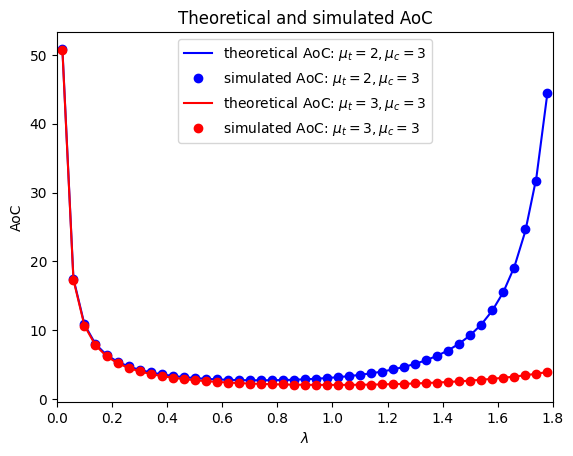
In Fig. 5, we compare theoretical and simulated average AoC under the soft deadline. The parameters are set as , , , and . The results show that the theoretical average AoC values derived in (2) and (2) closely match the simulation outcomes. This alignment implies that the theoretical expressions in Theorem 2 are accurate for both cases where and . Additionally, in both scenarios, the average AoC initially decreases and then increases. When , the computation capability exceeds the communication capability. If , the communication queue is almost empty, meaning that the communication resources (and thus the computation resources) are underutilized, resulting in a high average AoC. Conversely, if , the communication queue is busy, meaning that the communication capability is utilized almost to its total capacity, resulting in many tasks waiting in the communication queue to be transmitted, which also leads to a high average AoC. Since and are symmetric in (2) and (2), this conclusion is valid for the case when . Using numerical methods (e.g., gradient methods in as described in [31]), we can find the optimal in (2) and (2).
VI-B Simulations for AoC under the Hard Deadline
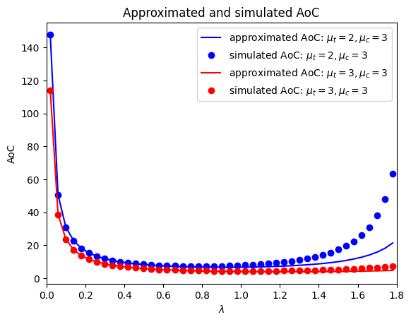
In Fig. 6, we investigate the average AoC under the hard deadline scenario. The comparisons between the approximated and simulated average AoC are presented in Fig. 6(a). We observe that when and , the approximations of the average AoC in (5) and (5) closely match the simulation results. This agreement verifies the theoretical expressions in Theorem 5. Furthermore, the curves of the approximated average AoC are below those of the simulated average AoC, implying that the approximations in (5) and (5) serve as lower bounds for the average AoC, confirming the validity of Remark 3. Additionally, in both scenarios, the average AoC initially decreases and then increases, similar to the trend observed under the soft deadline. This suggests that the computation freshness exhibits a convex relationship with respect to , indicating the existence of an optimal that minimizes the average AoC.
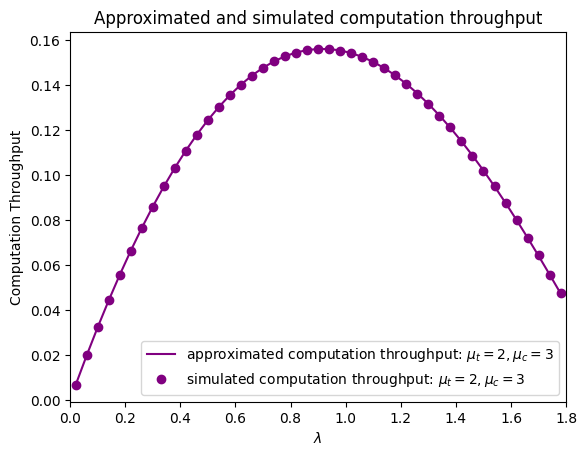
We analyze the computation throughput as defined in (18) in Fig. 6(b). The approximated computation throughput in (19) closely matches the simulated results, indicating the accuracy of the approximation. Although the positive correlations among are removed in (19), making it a lower bound, the reduction in the expectation of is small. Consequently, the reduction in is negligible. Therefore, (19) serves as a tight lower bound for the computation throughput, not only when and , but also across the entire range of .
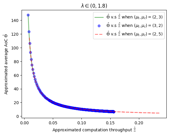
The relationship between the computation freshness and the computation throughput is examined in Fig. 7. In Fig. 7(a), we plot from (14) versus from (19) when and . These curves are observed to be decreasing, indicating that both and acheive their optimal values simutaneously. When the network is stable, i.e., , the channel throughput, defined as the number of completed tasks per slot, is . Fig. 7(a) shows that the approximated AoC decreases with the approximated computation throughput consistently. This suggests that computation throughput serves as a reliable proxy for the average AoC. Practically, we can minimize the average AoC by maximizing the computation throughput.
Additionally, the comparison of versus for (green solid line) aligns with that for (blue scatter line). This demonstrates that interchanging the communication and computation rates does not alter the relationship, highlighting the symmetry with respect to as discussed below Theorem 5. Comparing v.s when (the green solid line) with v.s when (the red dashed line), we observe that, for any fixed , the approximated computation throughput under is larger than that under . Similarly, the approximated average AoC under is smaller than that under . This is as expected because larger communication or computation capabilities lead to better computation freshness and higher throughput. Both the optimal approximated average AoC and approximated computation throughput for outperform those for due to the consistency between AoC and computation throughput.
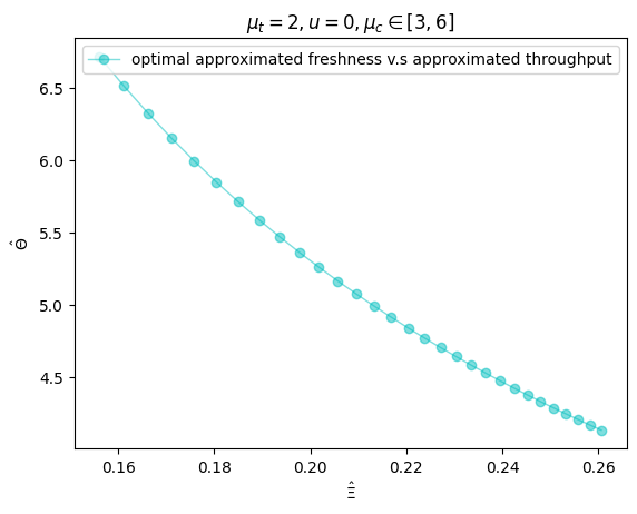
Finally, we solve the optimization (22) when , and plot the optimal v.s the corresponding in Fig. 7(b). We set , , allowing to vary from to . As expected, as the computation rate (representing the computation power of the network) increases, the optimal (approximated) average AoC decreases while the corresponding (approximated) computation throughput increases.
VI-C AoC-based Scheduling in Multi-Source Networks
In this subsection, we numerically validate the time-discrete and real-time Max-Weight scheduling policies proposed in Section V. As a benchmark, we compare them against stationary randomized policies [29]: Under these policies, when the receiver makes a scheduling decision, transmitter is selected with a fixed probability , and the receiver remains idle with a fixed probability . We consider a symmetric network, i.e., for all . The parameters are set as , , , , and . Given the network symmetry, we set and with .
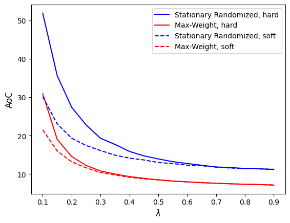
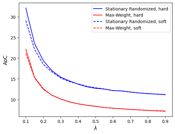
As shown in Fig. 8, the Max-Weight policy outperforms the benchmark stationary randomized policy, which is consistent with the findings in [29]. Unlike in Fig. 5 and Fig. 6(a), where the average AoC increases with , the average AoC in Fig. 8 decreases as increases. This difference arises because, in Fig. 5 and Fig. 6(a), the queuing discipline follows a first-come, first-serve (FCFS) rule, whereas Fig. 8 incorporates a preemptive rule. Under this rule, newly arrived tasks can replace previously queued tasks already present in the transmitter, which improves freshness.
Comparing Fig. 8(a) and Fig. 8(b), we observe that when is small (i.e., ), the average AoC under the hard deadline is higher than under the soft deadline. This is because fewer tasks are considered valid under the hard deadline, resulting in a higher AoC. However, when is large (i.e., ), most tasks remain valid, reducing the impact of on the AoC. Consequently, the difference in average AoC between the hard and soft deadlines becomes less significant.
VII Conclusion and Future Directions
In this paper, we introduce a novel metric AoC to quantify computation freshness in 3CNs. The AoC metric relies solely on tasks’ arrival and completion timestamps, ensuring its applicability to dynamic and complex real-world 3CNs. We investigate AoC in two distinct setting. In point-to-point networks: tasks are processed sequentially with a first-come, first-served discipline. We derive closed-form expressions for the time-average AoC under both a simplified case involving M/M/1-M/M/1 systems and a general case with G/G/1-G/G/1 systems. Additionally, we define the concept of computation throughput and derive its corresponding expressions. We further apply the AoC metric to resource optimization and real-time scheduling in time-discrete multi-source networks. In the multi-source networks: we propose AoC-based Max-Weight policies, leveraging a Lyapunov function to minimize its drift. Simulation results are provided to compare the proposed policies against benchmark approaches, demonstrating their effectiveness.
There are two primary future research directions: (1) Deriving and analyzing time-average AoC in practical scenarios involving complex graph structures, such as sequential dependency graphs, parallel dependency graphs, and general dependency graphs [1]. (2) Exploring optimal AoC-based resource management policies in dynamic and complex 3CNs, such as task offloading in mobile edge networks.
References
- [1] Y. Mao, C. You, J. Zhang, and et. al, “A Survey on Mobile Edge Computing: The Communication Perspective,” IEEE Communications Surveys and Tutorials, vol. 19, no. 4, pp. 2322–2358, 2017.
- [2] W. Shi, J. Cao, Q. Zhang, and et. al, “Edge Computing: Vision and Challenges,” IEEE Internet of Things Journal, vol. 3, no. 5, pp. 637–646, 2016.
- [3] Fog computing and its role in the internet of things. New York, NY, USA: Association for Computing Machinery, 2012.
- [4] X. Tang, C. Cao, and Y. Wang, “Computing power network: The architecture of convergence of computing and networking towards 6G requirement,” China Communications, vol. 18, no. 2, pp. 175–185, 2021.
- [5] A. Kosta, N. Pappas and V. Angelakis, “Age of Information: A New Concept, Metric, and Tool,” Foundations and Trends in Networking, vol. 12, no. 3, pp. 162 – 259, 2017.
- [6] X. Chen, K. Gatsis, H. Hassani and S. Saeedi-Bidokhti, “Age of Information in Random Access Channels,” IEEE Transactions on Information Theory, vol. 68, no. 10, pp. 6548 – 6568, 2022.
- [7] L. Huang and E. Modiano, “Optimizing age-of-information in a multiclass queueing system,” in IEEE International Symposium on Information Theory, 2015.
- [8] X. Chen, X. Liao, and S. Saeedi-Bidokhti, “Real-time Sampling and Estimation on Random Access Channels: Age of Information and Beyond,” in IEEE International Conference on Computer Communications, 2021.
- [9] Y. Zheng, J. Hu, and K. Yang, “Average Age of Information in Wireless Powered Relay Aided Communication Network,” IEEE Internet of Things Journal, vol. 9, no. 13, pp. 11 311 – 11 323, 2022.
- [10] X. Chen, R. Liu, S. Wang, and S. Saeedi-Bidokhti, “Timely Broadcasting in Erasure Networks: Age-Rate Tradeoffs,” in IEEE International Symposium on Information Theory, 2021.
- [11] X. Chen and S. Saeedi Bidokhti, “Benefits of Coding on Age of Information in Broadcast Networks,” in IEEE Information Theory Workshop, 2019.
- [12] Q. Kuang, J. Gong, X. Chen, et. al, “Age-of-information for computation-intensive messages in mobile edge computing,” in The 11th International Conference on Wireless Communications and Signal Processing, 2019.
- [13] C. Xu, H. H. Yang, X. Wang, et. al, “Optimizing information freshness in computing-enabled IoT networks,” IEEE Internet of Things Journal, vol. 2, no. 971 - 985, 2020.
- [14] F. Chiariotti, O. Vikhrova, B. Soret, et. al, “Peak age of information distribution for edge computing with wireless links,” IEEE Transactions on Communications, vol. 69, no. 5, pp. 3176 – 3191, 2021.
- [15] P. Zou, O. Ozel, and S. Subramaniam, “Optimizing information freshness through computation–transmission tradeoff and queue management in edge computing,” IEEE/ACM Transactions on Networking, vol. 29, no. 2, pp. 949 – 963, 2021.
- [16] X. Qin, Y. Li, X. Song, et. al, “Timeliness of information for computation-intensive status updates in task-oriented communications,” IEEE Journal on Selected Areas in Communications, vol. 41, no. 3, pp. 623 – 638, 2023.
- [17] Z. Tang, Z. Sun, N. Yang, et. al, “Age of information analysis of multi-user mobile edge computing systems,” in IEEE Global Communications Conference, 2021.
- [18] L. Liu, J. Qiang, Y. Wang, et. al, “Age of information analysis of NOMA-MEC offloading with dynamic task arrivals,” in IEEE the 14th International Conference on Wireless Communications and Signal Processing, 2022.
- [19] X. Chen, K. Li, and K. Yang, “Timely Requesting for Time-Critical Content Users in Decentralized F-RANs,” arXiv: 2407.02930, Jul 2024.
- [20] J. He, D. Zhang, S. Liu, et. al, “Decentralized updates scheduling for data freshness in mobile edge computing,” in IEEE International Symposium on Information Theory, 2022.
- [21] K. Peng, P. Xiao, S. Wang, et. al, “AoI-aware partial computation offloading in IIoT with edge computing: a deep reinforcement learning based approach,” IEEE Transactions on Cloud Computing, vol. 11, no. 4, pp. 3766 – 3777, 2023.
- [22] J. Zhong, R. D. Yates, and E. Soljanin, “Two freshness metrics for local cache refresh,” in IEEE International Symposium on Information Theory, 2018.
- [23] C. Kam, S. Kompella, G. D. Nguyen, et. al, “Towards an effective age of information: Remote estimation of a Markov source,” in IEEE Conference on Computer Communications Workshops, 2018.
- [24] A. Maatouk, S. Kriouile, M. Assaad, et. al, “The Age of Incorrect Information: A New Performance Metric for Status Updates,” IEEE/ACM Transactions on Networking, vol. 28, no. 5, pp. 2215 – 2228, 2020.
- [25] X. Zheng S. Zhou, and Z. Niu, “Beyond Age: Urgency of Information for Timeliness Guarantee in Status Update Systems,” in 2020 2nd 6G Wireless Summit, 2020.
- [26] S. Kaul, R. Yates, and M. Gruteser, “Real-Time Status: How Often Should One Update?” in IEEE International Conference on Computer Communications, 2012.
- [27] J. Lou, X. Yuan, S. Kompella, et.al, “AoI and throughput tradeoffs in routing-aware multi-hop wireless networks,” in IEEE Conference on Computer Communications, 2020.
- [28] M. T. M. Emmerich and A. H. Deutz, “A tutorial on multiobjective optimization: fundamentals and evolutionary methods,” Natural Computing, vol. 17, pp. 585 – 609, 2018.
- [29] I. Kadota and E. Modiano, “Minimizing the Age of Information in Wireless Networks with Stochastic Arrivals,” IEEE Transactions on Mobile Computing, vol. 20, no. 3, pp. 1173 – 1185, 2021.
- [30] M. J. Neely, Stochastic Network Optimization with Application to Communication and Queueing Systems. Morgan and Claypool Publishers, 2010.
- [31] S. Boyd, L. Vandenberghe, Convex Optimization. Cambridge University Press, 2004.
- [32] R. Nelson, Probability, stochastic processes, and queueing theory: the mathematics of computer performance modeling. Springer-Verlag New York, Inc., 1995.
Appendix A Proof of Theorem 1
Recall that represents the frequency of valid tasks and is identical across . The limit of exists and is denote by . We have:
Additionally, remains unchanged until a new task is completed. Consider the -th valid task, where the corresponding inter-arrival time is and the system time is . Let the corresponding value of be . We then have:
To derive an expression for the average AoC, we start with a similar graphical argument from [5]. Consider the sum of: (i) the area corresponding to the interval , i.e., the area of trapezoid , and (ii) the area corresponding to the additional latency incurred by task , i.e., the area of triangle in Fig. 2 (a), or the area of trapezoid in Fig. 2 (b). Note that . Denote the corresponding sum area as , based on Fig. 2, we can compute
| (32) |
Since , and are i.i.d, then and are also i.i.d, respectively.
Let the number of valid tasks be , and consider the limit as . Utilizing a similar graphical argument in Appendix A, the average AoC can be computed by
By the Law of Large Numbers, reduces to
| (33) |
Now, let us focus on the term . Since , for any small , there exists a large integer such that . Then:
The equality (a) holds because , as there are only finite number () terms and each term is a finite scalar.
Appendix B The proof of Theorem 2
First of all, we denote
From [16, Proposition 1], has the same formula of the average AoI, which has the following expression,
| (35) |
To obtain the closed expression for in (1), it suffices to obtain the closed expression for .
Step 1. We fisrt obtain . Denote and are the system in the transmission queue and the computation queue, respectively. Since the tandom is a combination of M/M/1 queues. Due to the momeryless property, and are independent [32, 16]. The densifty functions for and are given by [32]:
| (36) | ||||
| (37) |
Due to independence, the densifty function of the total system time, i.e., , is calculated by convolutional [32]:
| (38) |
Recall that . From (38), can be computed as
| (39) |
Step 2. We compute . We first consider the case when , we then consider the case when .
When , according to (38), we have
By some algebra,
Therefore, when ,
| (40) |
Next, when , according to (38), we have
| (41) |
Step 3. We compute by considering the waiting time in the computation queue, denoted as . We have the following relation:
According to [32], the waiting time in the computation queue, , follows the density function:
where is the Dirac delta function. Since and are independent, and are also independent. By convolution, we can derive the density function of . When , we have:
and
| (42) |
When , we have:
and
| (43) |
Appendix C Proof of Theorem 3
The proof is inspired by the proof of [16, Proposition 1].
We first divide the delay of task intto components:
where and denote the waiting times of task in the transmission and computation queues, respectively, while and represent the serive times of task in the transmission and computation queues, respectivey. From (1), can be re-written as
| (44) |
Note that is independent of and , with , , and . Therefore, to compute , it suffices to determine , , and . Denote , , , , and .
Step 1. To obtain , we proceed as follows:
| (45) |
Since represents the waiting time in the transmission queue, we have . Thus,
| (46) |
Substituting (46) into (45), we obtain:
Step 2. To obtain , we proceed as follows:
| (47) |
The rest of the step is to find .
We introduce another random variable, , which represents the inter-depature time associated with task in the transmission queue. Note that forms a Markov chain. By the chain rule,
which implies
and therefore,
Using the definition of density functions, we replace the probabilities with their respective density functions. Integrating with respect to on both sides, we have:
| (48) |
To obtain (48), we need to obtain and .
Recall is the waiting time of task in the computation queue, we have . Thus,
| (49) |
At the end of this step, we obtain . Define and as the probabilities that the transmission queue is busy or idle, respectively, upon the arrival of task . Then:
| (50) |
When , the inter-departure time of task and task in the transmission queue equals the service time of task . Thus:
| (51) | |||
| (52) |
When , consists of components: the service time of task , , and the interval between the arrival of task and the departure of task , denoted by . Hence:
| (53) |
where represents the convolution operation.
It follows that
| (54) |
From the definition of as , and using the result from [16, Appendix A], we obtain:
| (55) |
Substituting (53) and (C) into (53), we get:
| (56) |
Step 3. To obtain , , and . Note that . Then:
Substituting into , , and , we have
From Steps 1 3, we obtain the desired results.
Appendix D Proof of Theorem 4
Utilizing a similar idea of calculating average AoI [5], the average AoC can be computed as the sum of area of the parallelogram (e.g., ) over time horizon . The number of corresponding parallelograms is equal to the number of informative tasks. As the time horizon approaches infinity, the rate of informative tasks is
which is also the rate of parallelograms. Then, the average AoC is given by
| (57) |
From the distribution of in (IV-A), we know that a valid task followed by invalid tasks, so
| (58) |
In addition, the area of can be calculated by
| (59) |
Appendix E Proof of Theorem 5
As discussed in before, there are types of correlations underlying (13): (i) positive correlations among the delays over , (ii) positive correlations between () and , (iii) negative correlations between and , and (iv) negative correlations among and . The correlations in (ii), (iii), and (iv) are incurred by the positive correlations in (i). We can alleviate these correlations when the positive correlations in (i) are negligible.
In a tandem of two M/M/1 queues with parameters , when and , the positive correlations among become negligible [32]. In other words, and are approximately independent over . Consequently, due to the approximate independence among , according to (IV-A), approximates a geometric distribution with parameter , which is approximately independent of . Additionally, when and , the delay is dominated by the services times at the transmitter and the computational node. This implies that and are approximately independent. Hence, and are also approximately independent.
Step 1. We prove (14). Recall that are i.i.d over . As discussed above, when and , we have the following: (i) From the model assumption, are indepdent and identical distributions. Since is approximately independent of , we have:
| (60) | |||
| (61) |
(ii) Since is approximately independent of , we have:
| (62) |
Substituting (60), (61), and (62) into (13), we get:
thereby completing the proof of (14).
Step 2. We prove (5). According to (IV-A),
| (63) |
Since the density function of is given by (38), substituting (38) into (62), we have
| (64) |
Since has an exponential distribution with parameter , we have:
| (65) |
Recall that approximates a geometric distribution with parameter . Therefore,
| (66) |
where is gvien by (39). Substituting (39), (64), (65), and (66) into (14), we obtain (5).
Appendix F Proof of Lemma 1
Consider a large time horizon , during which there are informative packets. For each information task , denote the number of the associated bad tasks as . is identical over and follows the distribution given in (IV-A). Since are i.i.d over , the sequence are identical over . The remaining time in the interval is . Thus, the time horizon can be re-written as
| (68) |
Substituting (68) into (18), we have
Since the sequence is identical over , by the central limit theory, we have
Appendix G Proof of Proposition 1
Appendix H Proof of Lemma 2
The proof is based on contradiction. Assume that the pair is not a weakly Pareto-optimal point. This implies that there exists another solution such that and . Given that , the solution must be a feasible solution to problem (22). However, since is the minimum value in the problem (22), it follows that . This contradicts the assumption that .
Appendix I Proof of Theorem 6
In a tandem of two G/G/1 queues with parameters , when and , the positive correlations among become negligible [32]. In other words, and are approximately independent over . Consequently, due to the approximate independence among , and according to (IV-A), approximates a geometric distribution with parameter , which is approximately independent of . Additionally, when and , the delay is dominated by the services times at the transmitter and the computational node. This implies that and are approximately independent. Hence, and are also approximately independent. Based on the same process in Step 1 in Appendix E, we show that the average AoC defined in (13) can be accurately approximated by (14).
Step 1. The delay of task , , is the sum of the system times in both transmission and computation queues, i.e., . Based on Assumption 1, the density functions and are known. Denote the density function and CDF of as follows,
When and , the sequence is approximately independent. Therefore, from (IV-A), we have
| (70) |
Based on (I), it is straightforward to calculate,
| (71) | ||||
| (72) |
Appendix J Proof of Proposition 2
Appendix K Proof of (V-B1)
We first derive the recusion of with respect to . If a task from source with instantaneous is delivered to the receiver in time slot (i.e., ), then from (3), we have
where is defined in (3) and is defined in (4). Otherwise, if no task from source is delivered, we have:
Thus, the recursion for is given by:
| (74) |
where .
To schedule a transmitter in time slot , the receiver needs the network state in time slot :
-
•
If , meaning no task reaches the receiver in time slot , the receiver remains idle. Since a task takes at least 2 slots from starting transmission to leaving the computational node, no tasks from source can leave the computational node. Thus, from (K), we have .
-
•
If If , meaning a task is delivered to the receiver in time slot , but (i.e., transmitter is not scheduled in time slot ), then no tasks from source can leave the computational node. Thus, from (K), we have .
- •
Based on the discussion above, we can write the expression for as follows,