Algebro-geometric solutions to the lattice potential modified Kadomtsev–Petviashvili equation
Abstract
Algebro-geometric solutions of the lattice potential modified Kadomtsev–Petviashvili (lpmKP) equation are constructed. A Darboux transformation of the Kaup–Newell spectral problem is employed to generate a Lax triad for the lpmKP equation, as well as to define commutative integrable symplectic maps which generate discrete flows of eigenfunctions. These maps share the same integrals with the finite-dimensional Hamiltonian system associated to the Kaup–Newell spectral problem. We investigate asymptotic behaviors of the Baker–Akhiezer functions and obtain their expression in terms of Riemann theta function. Finally, algebro-geometric solutions for the lpmKP equation are reconstructed from these Baker–Akhiezer functions.
Key words: lattice potential modified Kadomtsev–Petviashvili equation, algebro-geometric solution, Kaup–Newell spectral problem, Baker–Akhiezer function
Mathematics Subject Classification (2000): 35Q51, 37K60, 39A36
1 Introduction
In recent two decades discrete integrable systems have undergone a true development (see [31] and the references therein). One of remarkable results is the Adler–Bobenko–Suris (ABS) classification of quadrilateral equations that are consistent around a cube (CAC) [52, 48, 5, 1] with certain extra restrictions (affine linear, D4 symmetry and tetrahedron property) [1]. The ABS list contains only 9 equations, named H1, H2, H, A, A2, Q, Q2, Q and Q4. The ABS equations serve as main objects in the study of discrete integrable systems, although many equations in the list are already found before. During the study, some methods have been developed or elaborated for discrete integrable systems, such as the Cauchy matrix approach [49, 63], bilinear method [32], inverse scattering transform [7] and algebraic geometry approach [9].
The finite-gap integration method was created for solving the Korteweg–de Vries (KdV) equation with periodic initial value problem by Novikov, Maveev and their collaborators Dubrovin, Its and Krichever in 1970s [20, 21, 34, 35, 42, 54]. The obtained periodic solutions are called finite-gap solutions or algebro-geometry solutions. After the original work, the theory has undergone a true development (e.g.[4, 28, 29]) and had a strong impact on the evolution of modern mathematics and theoretical physics (see [45] and the references therein for the historical review of finite-gap integration method).
For fully discrete equations, such as the ABS equations, algebro-geometry solutions have been derived from several equations in a series of papers [9, 10, 12, 13, 60, 61, 62] by Cao, Xu and their collaborators, which establish an algebro-geometric approach to periodic solutions for discrete equations that are multi-dimensionally consistent. This approach can be sketched as the following three steps. For a given quadrilateral equation which admits a Lax pair, in the first step we find an associated continuous spectral problem that is compatible with the discrete Lax pair. In step 2, consider the Hamiltonian system that arises from the associated continuous spectral problem and derive independent integrals of the Hamiltonian system. Then, view the discrete Lax pair as maps by which discrete flows of eigenfunctions can be generated. Using the compatibility between the maps and the associated continuous spectral problem, one can prove that the maps are symplectic and integrable in Liouville sense, sharing the same integrals with the Hamiltonian system. Finally, in step 3, using algebro-geometric technique, introduce Baker–Akhiezer functions and Abel–Jacobi variables, and express the Baker–Akhiezer functions in terms of the Riemann theta function according to their divisors, and recover the discrete potential functions which are expressed in terms of the Riemann theta function. The approach was also extended to the lattice potential Kadomtsev–Petviashvili (lpKP) equation [10] which is 4D consistent [2].
The first step of the approach is a starting point but it is highly nontrivial. In fact, since the Lax pair are compatible with the associated continuous spectral problem, the Lax pair can be considered as Darboux transformations of the continuous spectral problem (cf.[44]). With regard to an ABS equation, its spectral problem is thought to be a Darboux transformation of some continuous spectral problem, but such associated continuous spectral problems are still unknown for H2, H, Q2, Q and Q4. In this step, one needs to secure a continuous spectral problem and simultaneously to find a “suitable” Darboux transformation which not only can act as a spectral problem of the target discrete equation, but also can be used to recover the discrete potential functions in the follow-up steps. And moreover, the Darboux transformation is usually different from the discrete spectral problem obtained from multidimensional consistency. Of course, the step 2 and 3 are also different for different equations. Let us list out the associated continuous spectral problems that have been used in this approach. The Schrödinger spectral problem (in matrix form)
was used in [9] for solving H1. To solve Hirota’s discrete sine-Gordon equation, spectral problems
was employed [12]. Ref.[61] made use of
to solve Q. Ref.[62] solves H1, H and Q and the three associated continuous spectral problems are, respectively,
where the second one is known as the Kaup–Newell spectral problem. In [60], to solve Q, spectral problem
has been used. For the coupled lattice nonlinear Schrödinger equations, a nonsymmetric 3D lattice, and the lpKP equation, the Zakharov–Shabat–Ablowitz–Kaup–Newell–Segur (ZS–AKNS) spectral problem
| (1.1) |
was employed respectively in [13] and [10]. Note that one discrete equation may have more than one associated continuous spectral problems, e.g. H1 and Q.
This paper is devoted to finding algebro-geometric solutions to the lattice potential modified KP (lpmKP) equation,
| (1.2) |
where in the notation respectively stand for the numbers of continuous and discrete independent variables in the equation, are the lattice parameters associated with three directions , and are conventional notations denoting shifts in different directions, i.e.
This equation is first given in [50] (Eq.(4.16)), derived in a framework of direct linearisation for 3D lattice equations developed in [51]. It is one of the five octahedron-type equations that are 4D consistent [2]. In continuous limit the equation goes to the potential mKP equation [50]
| (1.3) |
The associated continuous spectral problem we will employ to solve the lpmKP equation is the KN spectral problem [36, 37]
| (1.4) |
The paper is organized as follows. In Section 2 we present a Lax triad for the lpmKP equation, explain connections between the Lax triad and the associated KN spectral problem. In Section 3, a nonlinear integrable symplectic map is obtained based on a finite-dimensional Hamiltonian system arising from the KN spectral problem. In Section 4, finite-gap solutions to the lpmKP equation (1.2) are constructed by introducing the Baker-Akhiezer functions and using a discrete analogue of the Liouville-Arnold theory. After that, we present an example of the obtained solutions for the case of genus one in Section 5. The concluding remarks are given in Section 6. We will also obtain a hierarchy of equations that are related to the lpmKP equation, in terms of the number of discrete independent variables. Together with some links between -dimensional and -dimensional integrable systems, these will be given in Appendix A. In addition, Appendix B provides some complex algebraic geometry preliminaries that will be used in our approach.
2 The lpmKP equation arising from compatibility
The idea of introducing discretisation by transform originated in [43, 44]. A Darboux transformation of a continuous spectral problem can serve as a discrete spectral problem to generate semi-discrete and fully discrete integrable systems, e.g. [14, 38, 41, 53, 64]. In this section, we will explain how the lpmKP equation (1.2) is connected with the KN spectral problem (1.4). These connections are important for us to reconstruct the discrete potential function in the follow-up sections.
Consider a Darboux transformation of the KN spectral problem (1.4): (cf.[64])
| (2.1) |
where serves as a soliton parameter, which transforms (1.4) to . This requires that111Considering (2.1) as a discrete spectral problem, equation (2.2) is the semi-discrete zero curvature equation from the compatibility between (2.1) and (1.4)
| (2.2) |
where we have taken
| (2.3a) | |||
| It follows that | |||
| (2.3b) | |||
| (2.3c) | |||
| (2.3d) | |||
which allows a special formulation222Note that this formulation is different from the Case in [64] and therefore the spectral problem (2.1) (with formulation (2.4)) is different from the spectral problem introduced in [59].
| (2.4a) | |||
| (2.4b) | |||
As a byproduct, equation (2.3b) (in terms of the variables ) provides a Bäcklund transformation for the KN potentials in (1.4),
| (2.5a) | |||
| (2.5b) | |||
which can also be regarded as a semi-discrete derivative nonlinear Schrödinger (dNLS) equation as it continuum limit yields the dNLS equation (A.4) (see Appendix A).
Remark 2.1.
Note that given in (2.4a) is one of roots of the quadratic equation , which results from the relation (2.3). If we take another root, , we will have an analogue of (2.5):
However, it cannot recover the continuous dNLS equation (A.4) in continuum limit due to the fatal minors sign in front of the square roots. In this context, in the paper we will only consider the consequential results of (2.4a).
Next, in order to derive the lpmKP equation (1.2), we consider discrete spectral problems, which are three replicas of equation (2.1) with the formulation (2.4),
| (2.6c) | |||
| (2.6f) | |||
| (2.6i) | |||
where stands for the shift operator in -direction, i.e. , serves as the spacing parameter of the -direction, and in light of (2.4a),
| (2.7) |
One can quickly check that the compatibility between (2.6c) and (2.6f) requires that
| (2.8) |
This relation, together with (2.3d), leads us to introducing
| (2.9) |
and
| (2.10a) | |||
| (2.10b) | |||
| (2.10c) | |||
Later in Section 4 we will derive in an explicit form, from which can be “integrated” from (2.10). In this sense, and act as auxiliary variables and is a dummy variable. Note that explicit and can also be obtained from (see Remark 4.1).
In order to show that defined by the triad (2.6) via (2.10) satisfies the lpmKP equation (1.2), we first look at equations resulting from the compatibility of the first two equations in (2.6).
Lemma 2.1.
Proof.
By making use of relation (2.8), the compatibility of equations (2.6c) and (2.6f) gives rise to
where and are given in (2.11). In addition, noticing that
| (2.13) |
we obtain equation (2.12) as a consequence of (2.11). The proof is then completed.
∎
Next, we can show that satisfies the lpmKP equation (1.2) after consistently introducing evolution in the third direction.
Theorem 2.1.
Proof.
In fact, in addition to the relation (2.13), compatibility between any two equations in the triad (2.6) yields
Then, noticing that
| (2.15) |
and replacing by using (2.10), we arrive at the lpmKP equation (1.2). The proof is completed.
∎
Since the spectral problem (2.6c) arises from the Darboux transformation (2.1), which commutes with the KN spectral problem and therefore may serve as a Darboux transformation for the whole KN hierarchy, we can have more equations in this frame, which have different number of discrete independent variables and compose a hierarchy of the lpmKP family. Since we will focus on the lpmKP equation (1.2), we will list out these semi-discrete equations in Appendix A.
3 Nonlinear integrable map
In this section, we will prove that the Darboux transformation (2.1) (with (2.3)) is an integrable symplectic map.
For the sake of self-containedness of the paper, let us recall some results given in [11] for the Hamiltonian system associated with the KN spectral problem (1.4). Let be any positive integer, , and with distinct and non-zero . A Liouville integrable Hamiltonian system is constructed by copies of the KN spectral problem (1.4), by imposing a constraint (3.1c) on , as
| (3.1a) | |||
| (3.1b) | |||
| (3.1c) | |||
where and . Note that equation (3.1c), coinciding with squared eigenfunction symmetry constraint, converts the KN spectral problem (1.4) to the Hamiltonian equation (3.1b), which is nonlinear with respect to the eigenfunction . Such a procedure is usually referred to as nonlinearisation of a Lax pair (cf.[8]). The associated Lax equation has a solution, which is
| (3.2) |
where . It satisfies the -matrix Ansatz [3, 22, 27]
| (3.3) |
where
This implies the Poisson commutativity , where (cf.[60]) and the Poisson bracket is defined as
The Hamiltonian can be determined by the expansion
| (3.4) |
which implies that . The generating function can be expanded as
| (3.5) |
which yields a complete set of integrals for the Hamiltonian system ,
| (3.6) |
where . Suppose that the roots of are , then we have the factorization
| (3.7) |
where . Thus a hyperelliptic curve
| (3.8) |
with genus , is defined. The Riemann surface where is consists of two sheets, and the curve is of hyperelliptic involution in the sense that maps to itself. For a non-branching point on the Riemann surface, when necessary, we distinguish the two corresponding points on by
| (3.9) |
and in particular, for the infinity on the Riemann surface, we denote the two corresponding points on by .
Generically [23, 30, 47] based on the curve (3.8), one can introduce Abelian differentials of the first kind, by which a Riemann theta function can be defined. One can refer to Appendix B for details.
Next, let us introduce our integrable map. Using the Darboux transformation (2.1) (with (2.3)), we define the following linear map:
| (3.10a) | |||
| (3.10b) | |||
The extra factor in front of is to make the determinant to be 1, which is useful in proving to be symplectic. One can convert the constraint (3.1c) on to be the following constraint on :
| (3.11a) | |||
| (3.11b) | |||
In fact, (3.11a) is nothing but
where in (2.3c) and have been used. To achieve (3.11b), one may start from the constraint and consider
Replacing by from (2.3c) and replacing using the map (3.10b), yield (3.11b).
In the following, by the nonlinearized map we mean the map (3.10) after imposing constraint (3.11) on . In fact, (3.11) indicates that can be explicitly expressed in terms of , which is denoted as
| (3.12a) | |||
| where | |||
| (3.12b) | |||
with where is defined by (3.7). Note that is single-valued in light of the monodromy formulation (3.9). So is . Thus, after replacing in (3.10) using (3.12b), the map is nonlinear with respect to .
Proposition 3.1.
The nonlinearized map is symplectic and Liouville integrable, sharing the same integrals , defined by equation (3.6), with the Hamiltonian system .
Proof.
Direct calculation from equation (3.10b) yields
| (3.13) |
which vanishes when constraint (3.11) makes sense. This means the map is symplectic. In addition, consider the Lax matrix given in equation (3.2) and the Darboux matrix given in (2.1). In light of the constraint (3.11), it turns out that
| (3.14) |
Thus , which indicates
| (3.15) |
It then follows from (3.5) that , which are invariants of the map .
∎
4 Algebro-geomitric solutions to the lpmKP equation
In this section we proceed to derive algebro-geometric solutions to the lpmKP equation (1.2).
First, using the integrable symplectic map (3.10), we define discrete phase flow with initial point , and then we use (3.12) to define finite genus potential in (2.1), i.e.
| (4.1) |
which coincides with . In light of (2.3), we also have
| (4.2a) | |||
| (4.2b) | |||
We will finally reconstruct in terms of theta function (see equation (4.25)) and by “integration” from (2.10) we recover the lpmKP solution .
Next, consider the discrete KN spectral problem (2.1) and the discrete Lax equation (3.14) along the -flow, which are rewritten as
| (4.3) |
and
| (4.4) |
where the Darboux matrix is
| (4.5) |
and is defined as the form (3.2). Let be a fundamental solution matrix of (4.3) with being the unit matrix . It turns out that
| (4.6a) | |||
| (4.6b) | |||
and we then have due to . For such an one can obtain its asymptotic behaviors from (4.6a).
Lemma 4.1.
and are polynomials of . When , for we have
| (4.7a) | ||||
| (4.7b) | ||||
| (4.7c) | ||||
| (4.7d) | ||||
and for they are still valid except . When , we have
| (4.8) |
Equation (4.4) indicates that the solution space of equation (4.3) is invariant under the action of the linear map . From (3.2), the traceless allows two opposite eigenvalues, denoted as , which are independent of the discrete argument due to relation (3.15). Denoting the corresponding eigenvectors by , we have
| (4.9a) | |||
| and | |||
| (4.9b) | |||
simultaneously. Noting that the rank of is 1, which means in each case the common eigenvector is uniquely determined up to a constant factor, we select two eigenvectors defined through , as the following,
| (4.10) |
where the constants are determined through (4.9a) and (4.6b), by
i.e. taking in equation (4.9a). It turns out that
| (4.11) |
Next, we will investigate these eigenvectors using the Baker–Akhiezer functions, which can be expressed by theta function on the hyperelliptic Riemann surface corresponding to the spectral curve . Let us introduce the Baker–Akhiezer functions, which are meromorphic on , by
| (4.12) |
To associate them with the Riemann theta function (see (B.8)), we investigate their analytic behaviors and divisors. To this end, introduce elliptic variables in and by
| (4.13a) | ||||
| (4.13b) | ||||
which lead us, from equations (4.6a) and (4.6b), to
| (4.14a) | |||
| (4.14b) | |||
With regard to asymptotic behaviors of the Baker–Akhiezer functions, we have the following lemmas.
Lemma 4.2.
The Baker–Akhiezer functions (4.12) have the following asymptotic behaviors as ,
| (4.15a) | |||
| (4.15b) | |||
| (4.15c) | |||
| (4.15d) | |||
Proof.
First, as we find from equations (4.11) and (3.2). Then, using (4.10) and the asymptotic results of given in Lemma 4.1, one can obtain (4.15a) and (4.15c). The other two in (4.15) follow from (4.14).
∎
Lemma 4.3.
When , the following asymptotic behaviors hold,
| (4.16a) | ||||
| (4.16b) | ||||
Proof.
From (4.11) we have as . Equations (4.8) and (4.10) yield (4.16a), which further gives rise to (4.16b) by using (4.14a).
∎
Now we are able to write down divisors of the Baker–Akhiezer functions on , which are, respectively, (cf.[23, 30, 47])
| (4.17a) | |||
| (4.17b) | |||
where , .
Next, introduce the Abel–Jacobi variables
| (4.18) |
by using the Abel map (see Appendix B). Employing Toda’s dipole technique [56], from (4.18) and (4.17) we have
| (4.19a) | ||||
| (4.19b) | ||||
| (4.19c) | ||||
Then, as usual treatment (cf.[9, 23, 30, 47]), by comparing divisors we obtain express the Baker-Akhiezer functions in terms of the Riemann theta function (B.8):
| (4.20a) | ||||
| (4.20b) | ||||
where and are constant factors and the Riemann constant vector is defined in (B.9). Here, is the dipole, a meromorphical differential that has only simple poles at and with residues and , respectively.
Our purpose is to derive explicit expression of in terms of the Riemann theta function. To achieve that, first, we take in equation (4.20b) and then compare the result with the asymptotic formula (4.15d). This gives rise to
| (4.21) |
where . Next, we consider the second row in equation (4.9b), i.e.
| (4.22) |
which reads
| (4.23) |
at the point since . Substituting (4.20b) with into (4.23) immediately yields
| (4.24) |
where . Now, substituting (4.21) into the above equation, we arrive at an explicit expression of in terms of theta function, i.e.
| (4.25) |
With in hand, for a function that obeys equation where is given in (4.25), one can obtain an explicit solution by “integration”,
| (4.26) |
Remark 4.1.
The above discussions and results are valid for , . Thus, we have three integrable symplectic maps and , which commute with each other since they share the same Liouville integrals (cf.[6, 12, 13, 57, 58]). This enables us to define
| (4.27) |
and the components satisfy the equation (3.10b) for simultaneously in the case of . This leads to a compatible solution
| (4.28) |
that satisfies the three equations in (2.6) with spectral parameter . Thus, one can obtain by “integrating” (2.6), and in light of Theorem 2.1, such provides solutions to the lpmKP equation (1.2).
5 An example: case
As an example of the solution (4.1), in the following we explore the simplest case, where genus . The elliptic curve (3.8) reads
| (5.1) |
with .
In our example, we assume all are on real axis and so that related branch cuts are taken as and . Thus, we have the Abelian differential of the first kind
| (5.2) |
where the normalization constant is
| (5.3) |
along with an -period. Then we have the two periods
| (5.4a) | ||||
| (5.4b) | ||||
Note that by certain linear fractional transformation (see [56]) the above two formulae can be converted to the elliptic integrals of the first kind:
| (5.5a) | ||||
| (5.5b) | ||||
where is a constant.
In this case the Riemann theta function reduces to the Jacobi theta function ,
| (5.6) |
Hence, the algebro-geometric solution (4.1) in the case of can be expressed as
| (5.7) |
where
| (5.8a) | |||
| (5.8b) | |||
| (5.8c) | |||
Note that due to the arbitrariness of we can always vanish and thus we come to
| (5.9a) | ||||
| with | ||||
| (5.9b) | ||||
| (5.9c) | ||||
where and are computed from (5.8b), and acts as a linear background of .
To illustrate the solution, we take
| (5.10) |
and consequently,
It follows from (5.3), (5.4) and (5.8) that (the integrals are computed numerically using Mathematica)
| (5.11) |
where we have taken in (5.8). The quasi-periodic evolution of is shown in Figure 1.
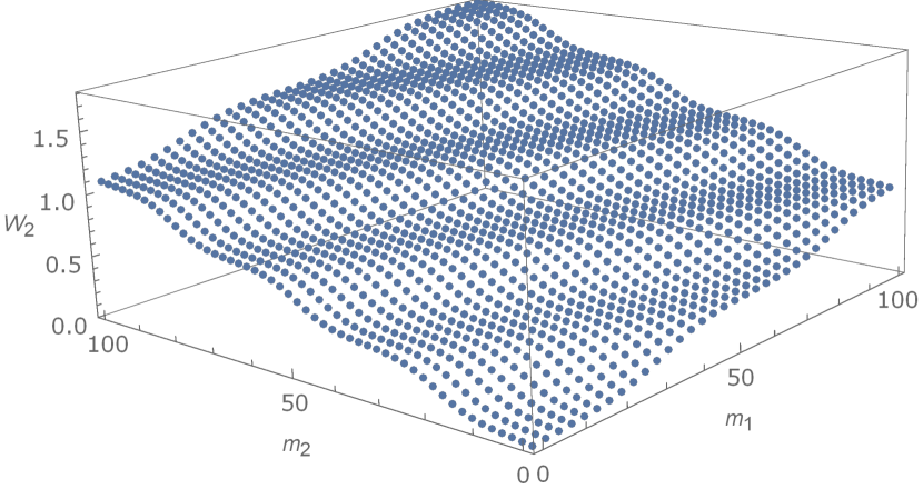
(a)
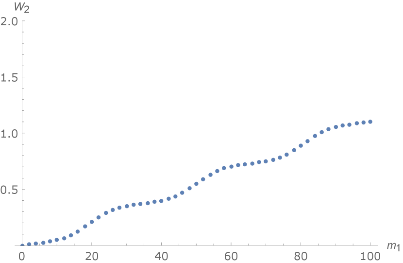
(b)
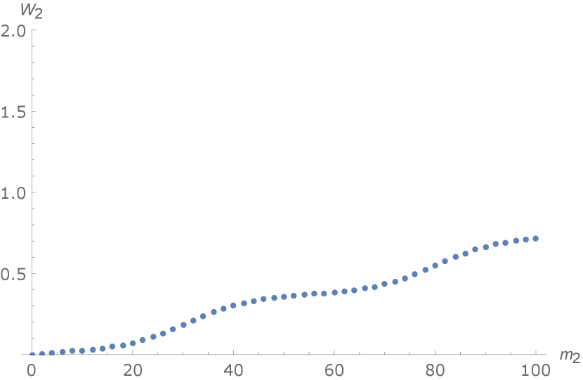
(c)
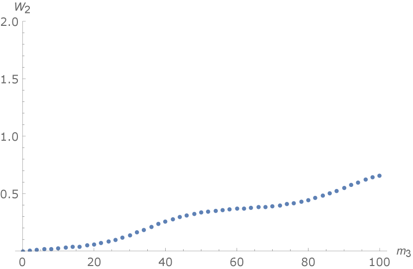
(d)
One can see a periodic wave coupled with an apparent linear background that is different from . This is because in our example all and are pure imaginary and Jacobi’s function has a -dependent periodic multiplier with respect to , i.e.
It is the periodic multiplier to give rise to the linear background when evolves with respect to via the formula (5.9b).
6 Concluding remarks
In this paper we constructed algebro-geometric solutions (4.1) to the lpmKP equation (1.2). The KN spectral problem (1.4) was employed as an associated spectral problem, of which the Darboux transformation gives rise to the Lax triad (2.6) for the lpmKP equation. Compared with the known one (e.g. Eq.(3.113) in [31]), this Lax triad is not explicit, as the discrete potential function is defined (via ) by the KN functions . Discrete evolutions are introduced by regarding the Darboux transformation as a map (3.10) to generate discrete flows. The map is shown to be symplectic and integrable, sharing the same integrals with the continuous Hamiltonian system (3.1) which is obtained through the so-called nonlinearisation of the KN spectral problem. Then, employing algebro-geometric techniques, using the Baker–Akhiezer functions and Abel map we introduced the Riemann theta function and finally obtained the algebro-geometric solutions (4.1) for the lpmKP equation. As an example, in Sec.5 we presented an explicit solution for the case and illustrated it in Fig.1.
Based on a series of work [9, 10, 12, 13, 60, 61, 62], in Sec.1 we have summarized a framework of the approach for constructing algebro-geometric solutions to multidimensionally consistent systems. The approach has proved effective and this paper added one more important successful example. Reviewing the series of work [9, 10, 12, 13, 60, 61, 62] and the present paper, there are several related problems that are interesting and remain open. Let us raise them below.
One is to extend solutions to full space. In fact, in the solutions (4.1) all , i.e. the solutions are defined on the first octant. The same thing happened to the lpKP equation [10]. For those quadrilateral equations studied in [9, 12, 13, 60, 61, 62], the obtained algebro-geometric solutions are defined on the first quadrant. This is because in this approach discrete flows are generated by iterating maps (e.g. (3.10)) towards one direction. One may develop the approach to obtain solutions in full space.
The second is to construct algebro-geometric solutions containing two soliton parameters for 3D lattice equations. Let us explain the problem below. In general, an integrable 3D equation admits a plane-wave factor (PWF) with two independent soliton parameters. For example, for the discrete AKP equation, its PWF reads [46]
where are spacing parameters and and are referred to as soliton parameters. By imposing constraints on one can have a PWF for reduced (2D) equations. Both the lpKP and lpmKP equations allow a PWF with two independent soliton parameters (§9.7 of [31]), and for 2D lattice equations, e.g. the ABS equations, their PWF usually reads [32, 49]
which contains only one soliton parameter . In the present paper, the lpmKP equation (1.2) is reconstructed in (2.15), as a consequence of 3D consistency of the ldNLS equation (2.11). Note that this does not mean the lpmKP equation (1.2) is a fake 3D equation, because it does allows PWF with two independent soliton parameters (§9.7 of [31]). However, this indicates that the solutions we constructed in the paper, by using 3D consistency of the 2D ldNLS equation, is a special solution in which PWF contains a single soliton parameter. One may develop an approach for 3D lattice equations to construct their algebro-geometric solutions in which the PWF contains two independent soliton parameters and therefore allows reductions.
The third problem is to apply the scheme to other ABS equations and 3D lattice equations that are 4D consistent (including octahedron-type equations [2] and the discrete BKP and Schwarzian BKP equation [1]). The approach has proved effective and so far H1, H3(0) and Q, lpKP and lpmKP have been solved with this approach. However, as we mentioned in Section 1, for other equations, the associated continuous spectral problems are still unknown. It is also notable that, as we pointed out in Section 1, for H1, H3(0) and Q, each equation can have more than one associated continuous spectral problems. For the same equation, these continuous spectral problems may lead to either same (for H1 and Q, cf.[9, 62], and cf. [61, 62]) or different hyperelliptic curves (for H, cf.[12, 62]), but for each equation the obtained solutions have different formulations.
The final problem is finite-gap integration based on theory of trigonal curves for discrete integrable systems. So far the hyperelliptic curves associated with the two-sheeted Riemann surfaces were employed in our scheme, cf.[9, 12, 13, 60, 61, 62]. There were already some exciting developments in the finite-gap integration theory based on trigonal curves in continuous case, e.g. [19, 24, 25, 26]. It would be very meaningful to develop the theory in discrete case to study lattice equations related to third-order spectral problem, e.g. the discrete Boussinesq equations [33].
Acknowledgments
The authors are grateful to the referees for their invaluable comments. Our sincere thanks are also extended to Dr. Xing Li for sharing her expertise of computing path integrations on torus and providing figures of this paper. This work is supported by the National Natural Science Foundation of China (grant nos. 11631007, 11875040).
Appendix A The semi-discrete lpmKP and ldNLS equations
Since the spectral problem (2.6c) arises from the Darboux transformation (2.1), which commutes with the KN spectral problem and may serve as a Darboux transformation for the whole KN hierarchy, we can have more equations in this frame, which compose a hierarchy of the lpmKP family, in terms of the number of discrete independent variables.
The first semi-discrete lpmKP equation (with two discrete independent variables) is
| (A.1) |
which is a consequence of the compatibility of (1.4) (2.6c) and (2.6f), where (2.10a), (2.10b) and (2.9) should be used. Alternatively, equation (A.1) is obtained from (2.12) by substituting (2.9) into the equation. Note that (A.1) was also found in [50] (Eq.(4.27)) as a continuum limit of the lpmKP equation (1.2).
The second semi-discrete lpmKP equation (with one discrete independent variable),
| (A.2) |
is obtained from the compatibility of (1.4), (2.6c) and the following linear problem
| (A.3) |
The calculation is complicated. Let us sketch it below. First, the compatibility of (1.4) and (A.3) yields the dNLS equations
| (A.4) |
and the compatibility of (1.4) and (A.3) yields relations (2.3) with formulation (2.4), where we need to replace with . In particular, (2.3b) and (2.3c) indicate that
| (A.5) |
Then, making use of (2.9), (A.4) and (A.5), the compatibility of (2.6c) and (A.3) yields
which gives rise to equation (A.2). Note that (A.2) can also be derived in the following alternative way. From the first equation in (A.4) and the shifted second equation , one can have
| (A.6) |
which can lead to equation (A.2) by using (A.5) and relation due to . We also note that equation (A.2) can be converted to its non-potential form
| (A.7) |
where and . This equation was obtained in [55] as a gauge equivalence of a semi-discrete KP equation.
We have derived the lpmKP equation and two semi-discrete lpmKP equations and . All these equations have the pmKP equation (1.3), , as continuum limit. Let us replace by , with non-zero and distinct constants , and consider continuum limits in terms of Miwa’s variables , where [46]
This indicates that
where and for ; and for differential-difference case,
where and for ;
where and . It turns out that
Similarly, equations (2.5) and (2.11), up to some transformations, yield the dNLS equations (A.4) in continuum limit. In fact, for equation (2.5), we first replace and by , and , respectively, and rewrite (2.5) as
which is available for taking continuum limit. Then, let and define
where and . Then we have
where are given in (A.4). Finally, in (2.11), replace by and by , and rewrite the equation as
Let and introduce
where and for . The continuum limit yields
In the rest part of this section, we review some links between -dimensional and -dimensional integrable systems, which maybe helpful for understanding the connections in the discrete case. Let us start with the continuous mKP hierarchy, which are generated from the compatibility of (see [39])
| (A.8a) | |||
| (A.8b) | |||
where , , stands for the pure differential part of . One can express for in terms of using the compatibility between (A.8a) and , and then the mKP hierarchy arise from the compatibility of and (A.8b). By we denote the operator adjoint of . Introduce
| (A.9) |
It can be verified that for the above eigenfunctions and , the mKP hierarchy admits a symmetry . Consider the symmetry constraint . In the following we denote and , thus we have (cf. in (2.9))
| (A.10) |
With this constraint, the spectral problem (A.8a) is converted to the KN spectral problem (1.4) (up to gauge transformation), and the coupled system (A.8b) and (A.9) (with ) give rise to the KN hierarchy (up to gauge transformation)
| (A.11) |
For more details, one may refer to [15]. Note that the KN hierarchy (A.11) also result from the compatibility of the KN spectral problem (1.4) and the time evolution . In this context, it is not surprised that the potential mKP equation (1.3) can be obtained from the compatibility of the triad for and with and . Such a link between -dimensional and -dimensional integrable systems was first revealed in [8, 18, 40] in the early 1990s for the ZS-AKNS and KP systems. For the differential-difference case with one discrete independent variable, the analogue results build connections between the semi-discrete ZS-AKNS and differential-difference KP systems (see [16]). The obtained semi-discrete ZS-AKNS spectral problem is nothing but the Darboux transformation of the ZS-AKNS spectral problem (1.1), and it has been used to derive algebro-geometry solutions for the lpKP equation [10]. However, for the differential-difference mKP hierarchy, its eigenfunction symmetry constraint gives rise the relativistic Toda spectral problem (see [17]), which is not the Darboux transformation (2.1) that we used in this paper. Anyway, as we can see, in our approach it is an important step to establish the link between the lpmKP and KN equations. The eigenfunction symmetry constraint can provide some insights but not always as direct as expected.
Appendix B Riemann theta function associated with hyperelliptic curve
In this section we introduce how a Riemann theta function arises from a hyperelliptic curve. For more details one can refer to [23, 30, 47]. This section also provides some complex algebraic geometry preliminaries that will be used in our approach.
For a generic hyperelliptic curve : with genus (for example, (3.8)), the following Abelian differentials of the first kind constitute the basis of holomorphic differentials of :
| (B.1) |
Let the closed loops be the canonical basis of the homology group , with intersection numbers
Note that here we adopt the conventional notations for these canonical basis, without making confusion with the discrete potentials that we used in Sec.4. The basis of holomorphic differentials can be normalized as follows:
| (B.2) | ||||
where
| (B.3) |
and stands for the l-th column vector of . For this normalized basis , we have
| (B.4) |
where the matrix is symmetric with positive definite imaginary part. can be used as a periodic matrix to defined the Riemann theta function (which is holomorphic):
| (B.5) |
where by we denote the scalar product in .
Next, let us reveal features of zeros of the above Riemann theta function. Let be a period lattice }. The quotient space is called the Jacobian variety of . Introduce the Abel map (also called Abel-Jacobi map) , by
| (B.6) |
where with being some choosing fixed point. The map can be extended to the divisors by defining
| (B.7) |
Consider the function
| (B.8) |
where the divisor with being distinct points on , and the vector of Riemann constants is defined as
| (B.9) |
where is the -th component of the Abel map , and is the base point of the fundamental group (see [23]). By choosing , the above formula reduces to
| (B.10) |
According to the Riemann vanishing theorem, the zeros of are . Due to this fact, the Riemann theta function (B.8) is often used to characterize meromorphic functions with certain zeros and poles.
References
- [1] Adler, V.E., Bobenko, A.I., Suris, Yu.B.: Classification of integrable equations on quad-graphs. The consistency approach. Commun. Math. Phys. 233, 513–543 (2003)
- [2] Adler, V.E., Bobenko, A.I., Suris, Yu.B.: Classiffication of integrable discrete equations of octahedron type. Int. Math. Res. Not. 2012, 1822–1889 (2012)
- [3] Babelon, O., Bernard, D., Talon, M.: Introduction to Classical Integrable Systems. Camb. Univ. Press, Cambridge (2003)
- [4] Belokolos, E.D., Bobenko, A.I., Enolskij, V.Z., Its, A.R., Matveev, V.B.: Algebro-geometric Approach to Nonlinear Integrable Equations. Spinger, Berlin (1994)
- [5] Bobenko, A.I., Suris, Yu.B.: Integrable systems on quad-graphs, Int. Math. Res. Not. 2002, 573–611 (2002)
- [6] Bruschi, M., Ragnisco, O., Santini, P.M., Tu, G.Z.: Integrable symplectic maps. Phys. D 49, 273–294 (1991)
- [7] Butler, S.: Multidimensional inverse scattering of integrable lattice equations. Nonlinearity 25, 1613–1634 (2012)
- [8] Cao, C.W.: Nonlinearization of the Lax system for AKNS hierarchy. Sci. China Ser. A 33, 528–536 (1990)
- [9] Cao, C.W., Xu, X.X.: A finite genus solution of the H1 model. J. Phys. A: Math. Theor. 45, 055213 (2012)
- [10] Cao, C.W., Xu, X.X., Zhang, D.J.: On the lattice potential KP equation. In: Nijhoff F.W., Shi Y., Zhang D.J. (eds), Asymptotic, Algebraic and Geometric Aspects of Integrable Systems, Springer Proceedings in Mathematics Statistics, vol. 338. Springer, Cham (2020)
- [11] Cao, C.W, Yang, X.: A (2+1)-dimensional derivative Toda equation in the context of the Kaup–Newell spectral problem. J. Phys. A: Math. Theor. 41, 025203 (2008)
- [12] Cao, C.W., Zhang, G.Y.: A finite genus solution of the Hirota equation via integrable symplectic maps. J. Phys. A: Math. Theor. 45, 095203 (2012)
- [13] Cao, C.W., Zhang, G.Y.: Integrable symplectic maps associated with the ZS-AKNS spectral problem. J. Phys. A: Math. Theor. 45, 265201 (2012)
- [14] Cao, C.W., Zhang, G.Y.: Lax pairs for discrete integrable equations via Darboux transformations. Chin. Phys. Lett. 29, 050202 (2012)
- [15] Chen, D.Y.: -constraint for the modified Kadomtsev–Petviashvili system. J. Math. Phys. 43, 1956–1965 (2002)
- [16] Chen, K., Deng, X., Zhang, D.J.: Symmetry constraint of the differential-difference KP hierarchy and a second discretization of the ZS–AKNS system. J. Nonl. Math. Phys. 24(Suppl.1), 18–35 (2017)
- [17] Chen, K., Zhang, C. Zhang D.J.: Squared eigenfunction symmetry of the DmKP hierarchy and its constraint, Stud. Appl. Math. 147, 752–791 (2021)
- [18] Cheng, Y., Li Y.S.: The constraint of the Kadomtsev–Petviashvili equation and its special solutions. Phys. Lett. A. 157, 22–26 (1991)
- [19] Dickson, R., Gesztesy, F., Unterkofler, K.: Algebro-geometric solutions of the Boussinesq hierarchy. Rev. Math. Phys. 11, 823–879 (1999)
- [20] Dubrovin, B.A.: Periodic problems for the Korteweg–de Vries equation in the class of finite band potentials. Funct. Anal. Appl. 9, 215–223 (1975)
- [21] Dubrovin, B.A., Novikov, S.P.: Periodic and conditionally periodic analogs of the many soliton solutions of the Korteweg-de Vries equation. Soviet Phys. JETP 40, 1058–1063 (1975)
- [22] Faddeev, L.D., Takhtajan, L.A.: Hamiltonian Methods in the Theory of Solitons. Springer, Berlin (1987)
- [23] Farkas, H.M., Kra, I.: Riemann Surfaces. Springer, New York (1992)
- [24] Geng, X.G., Wu, L.H., He, G.L.: Algebro-geometric constructions of the modified Boussinesq flows and quasi-periodic solutions. Phys. D 240, 1262–1288 (2011)
- [25] Geng, X.G., Wu, L.H., He, G.L.: Quasi-periodic solutions of the Kaup–Kupershmidt hierarchy. J. Nonlinear Sci. 23, 527–555 (2013)
- [26] Geng, X.G., Zhai, Y.Y., Dai, H.H.: Algebro-geometric solutions of the coupled modified Korteweg–de Vries hierarchy. Adv. Math. 263, 123–153 (2014)
- [27] Gerdjikov, V.S., Vilasi, G., Yanovski, A.B.: Integrable Hamiltonian Hierarchies. Springer, Berlin (2008)
- [28] Gesztesy, F., Holden, H.: Soliton Equations and Their Algebro-geometric Solutions: (1+1)-Dimensional Continuous Models. Camb. Univ. Press, Cambridge (2003)
- [29] Gesztesy, F., Holden, H., Michor, J., Teschl, G.: Soliton Equations and There Algebro-geometric Solutions. Volume II: (1+1)-Dimensional Discrete Models. Camb. Univ. Press, Cambridge (2009)
- [30] Griffiths, J.P., Harris, J.: Principles of Algebraic Geometry. Wiley, New York (1978)
- [31] Hietarinta, J., Joshi, N., Nijhoff, F.W.: Discrete Systems and Integrability. Camb. Univ. Press, Cambridge (2016)
- [32] Hietarinta, J., Zhang, D.J.: Soliton solutions for ABS lattice equations: II. Casoratians and bilinearization. J. Phys. A: Math. Theor. 42, 404006 (2009)
- [33] Hietarinta, J., Zhang, D.J.: Discrete Boussinesq-type equations. In Euler N., Zhang D.J. (eds.), Nonlinear Systems and Their Remarkable Mathematical Structures, Vol.3. CRC Press, Taylor & Francis, Boca Raton (2021)
- [34] Its, A.R., Matveev, V.B.: Hill operators with a finite number of lacunae. Funct. Anal. Appl. 9, 65–66 (1975)
- [35] Its, A.R., Matveev, V.B.: Schrödinger operators with the finite-band spectrum and the N-soliton solutions of the Korteweg–de Vries equation. Theor. Math. Phys. 23, 343–355 (1975)
- [36] Kaup, D.J., Newell, A.C.: On the Coleman correspondence and the solution of the massive Thirring model. Lett. AL Nuovo Cimento 20, 325–331 (1977)
- [37] Kaup, D.J., Newell, A.C.: An exact solution for a derivative nonlinear Schrödinger equation. J. Math. Phys. 19, 798–801 (1978)
- [38] Khanizadeh, F., Mikhailov, A.V., Wang, J.P.: Darboux transformations and recursion operators for differential-difference equations. Theore. Math. Phys. 177, 1606–1654 (2013)
- [39] Konopelchenko, B.G., Strampp, W.: New reductions of the Kadomtsev–Petviashvili and two-dimensional Toda lattice hierarchies via symmetry constraints, J. Math. Phys. 33, 3676–3686 (1992)
- [40] Konopelchenko, B.G., Sidorenko, J., Strampp, W.: (1+1)-dimensional integrable systems as symmetry constraints of (2+1)-dimensional systems. Phys. Lett. A 157, 17–21 (1991)
- [41] Konstantinou-Rizos, S., Mikhailov, A.V., Xenitidis, P.: Reduction groups and related integrable difference systems of nonlinear Schrödinger type. J. Math. Phys. 56, 082701 (2015)
- [42] Krichever, I.M.: Methods of algebraic geometry in the theory of non-linear equations. Russ. Math. Surv. 32, 185–213 (1977)
- [43] Levi, D.: Nonlinear differential-difference equations as Bäcklund transformations. J. Phys. A: Math. Gen. 14, 1083–1098 (1981)
- [44] Levi, D., Benguria, R.: Bäcklund transformations and nonlinear differential-difference equations. Proc. Nati. Acad. Sci. USA 77, 5025–5027 (1980)
- [45] Matveev, V.B.: 30 years of finite-gap integration theory. Phil. Trans. R. Soc. A 366, 837–875 (2008)
- [46] Miwa, T.: On Hirota’s difference equations. Proc. Japan Acad. Ser. A Math. Sci. 58, 9–12 (1982)
- [47] Mumford, D.: Tata Lectures on Theta I. Birkhäuser, Boston (1983)
- [48] Nijhoff, F.W.: Lax pair for the Adler (lattice Krichever–Novikov) system. Phys. Lett. A 297, 49–58 (2002)
- [49] Nijhoff, F.W., Atkinson, J., Hietarinta, J.: Soliton solutions for ABS lattice equations: I. Cauchy matrix approach. J. Phys. A: Math. Theor. 42, 404005 (2009)
- [50] Nijhoff, F.W., Capel, H., Wiersma, G.: Integrable lattice systems in two and three dimensions. In: Martini R. (ed.), Geometric Aspects of the Einstein Equations and Integrable Systems, Lecture Notes in Physics, vol. 239. Springer, Berlin, Heidelberg (1985)
- [51] Nijhoff, F.W., Capel, H., Wiersma, G., Quispel, G.R.W.: Bäcklund transformations and three-dimensional lattice equations. Phys. Lett. A 105, 267–272 (1984)
- [52] Nijhoff, F.W., Walker, A.J.: The discrete and continuous Painlevé VI hierarchy and the Garnier systems. Glasgow Math. J. 43A, 109–123 (2001)
- [53] Nimmo, J.J.C.: Darboux transformations and the discrete KP equation. J. Phys. A: Math. Gen. 30, 8693–8704 (1997)
- [54] Novikov, S.P.: The periodic problem for the Korteweg–de vries equation. Funct. Anal. Its Appl. 8, 236–246 (1974)
- [55] Tamizhmani, K.M., Kanaga Vel, S.: Gauge equivalence and -reductions of the differential-difference KP equation. Chaos Solitons Fractals 11, 137–143 (2000)
- [56] Toda, M.: Theory of Nonlinear Lattices. Springer, Berlin (1981)
- [57] Veselov, A.P.: Integrable maps. Russ. Math. Surv. 46, 3–45 (1991)
- [58] Veselov, A.P.: What is an integrable mapping?. In: Zakharov V.E. (ed.), What Is Integrability?. Springer-Verleg, Berlin, Heidelberg (1991)
- [59] Wu, Y.T., Geng, X.G.: A new hierarchy of integrable differential-difference equations and Darboux transformation. J. Phys. A: Math. Gen. 31, L677–L684 (1998)
- [60] Xu, X.X., Cao, C.W., Nijhoff, F.W.: Algebro-geometric integration of the Q1 lattice equation via nonlinear integrable symplectic maps. Nonlinearity 34, 2897–2918 (2021)
- [61] Xu, X.X., Cao, C.W., Zhang, G.Y.: Finite genus solutions to the lattice Schwarzian Korteweg–de Vries equation. J. Nonl. Math. Phys. 27, 633–646 (2020)
- [62] Xu, X.X., Jiang, M.M., Nijhoff, F.W.: Integrabe symplectic maps associated with discrete Korteweg–de Vries-type equations. Stud. Appl. Math. 146, 233–278 (2021)
- [63] Zhang, D.J., Zhao, S.L.: Solutions to ABS lattice equations via generalized Cauchy matrix approach. Stud. Appl. Math. 131, 72–103 (2013)
- [64] Zhou, R.G., Chen, J.: Two hierarchies of new differential-difference equations related to the Darboux transformations of the Kaup–Newell hierarchy. Commun. Theor. Phys. 63, 1–6 (2015)