Algorithms for Jumbled Pattern Matching in Strings
Abstract
The Parikh vector of a string over a finite ordered alphabet is defined as the vector of multiplicities of the characters, , where Parikh vector occurs in if has a substring with . The problem of searching for a query in a text of length can be solved simply and worst-case optimally with a sliding window approach in time. We present two novel algorithms for the case where the text is fixed and many queries arrive over time.
The first algorithm only decides whether a given Parikh vector appears in a binary text. It uses a linear size data structure and decides each query in time. The preprocessing can be done trivially in time.
The second algorithm finds all occurrences of a given Parikh vector in a text over an arbitrary alphabet of size and has sub-linear expected time complexity. More precisely, we present two variants of the algorithm, both using an size data structure, each of which can be constructed in time. The first solution is very simple and easy to implement and leads to an expected query time of , where is the length of a string with Parikh vector . The second uses wavelet trees and improves the expected runtime to , i.e., by a factor of .
Electronic version of an article accepted for publication in the International Journal of Foundations of Computer Science (IJFCS), to appear in 2011 ©World Scientific Publishing Company, www.wordscinet.com/ijfcs/
Keywords: Parikh vectors, permuted strings, pattern matching, string algorithms, average case analysis, text indexing, non-standard string matching
1 Introduction
Parikh vectors of strings count the multiplicity of the characters. They have been reintroduced many times by different names (compomer [5], composition [3], Parikh vector [22], permuted string [7], permuted pattern [10], and others). They are natural objects to study, due to their numerous applications; for instance, in computational biology, they have been applied in alignment algorithms [3], SNP discovery [5], repeated pattern discovery [10], and, most naturally, in interpretation of mass spectrometry data [4]. Parikh vectors can be seen as a generalization of strings, where we view two strings as equivalent if one can be turned into the other by permuting its characters; in other words, if the two strings have the same Parikh vector.
The problem we are interested in here is answering the question whether a query Parikh vector appears in a given text (decision version), or where it occurs (occurrence version). An occurrence of is defined as an occurrence of a substring of with Parikh vector . The problem can be viewed as an approximate pattern matching problem: We are looking for an occurrence of a jumbled version of a query string , i.e. for the occurrence of a substring which has the same Parikh vector. In the following, let be the length of the text , the length of the query (defined as the length of a string with Parikh vector ), and the size of the alphabet.
The above problem (both decision and occurrence versions) can be solved with a simple sliding window based algorithm, in time and additional storage space. This is worst case optimal with respect to the case of one query. However, when we expect to search for many queries in the same string, the above approach leads to runtime for queries. To the best of our knowledge, no faster approach is known. This is in stark contrast to the classical exact pattern matching problem, where all exact occurrences of a query pattern of length are sought in a text of length . In that case, for one query, any naive approach leads to runtime, while quite involved ideas for preprocessing and searching are necessary to achieve an improved runtime of , as do the Knuth-Morris-Pratt [17], Boyer-Moore [6] and Boyer-Moore-type algorithms (see, e.g., [2, 14]). However, when many queries are expected, the text can be preprocessed to produce a data structure of size linear in , such as a suffix tree, suffix array, or suffix automaton, which then allows to answer individual queries in time linear in the length of the pattern (see any textbook on string algorithms, e.g. [23, 18]).
1.1 Related work
Jumbled pattern matching is a special case of approximate pattern matching. It has been used as a filtering step in approximate pattern matching algorithms [15], but rarely considered in its own right.
The authors of [7] present an algorithm for finding all occurrences of a Parikh vector in a runlength encoded text. The algorithm’s time complexity is , where is the length of the runlength encoding of . Obviously, if the string is not runlength encoded, a preprocessing phase of time has to be added. However, this may still be feasible if many queries are expected. To the best of our knowledge, this is the only algorithm that has been presented for the problem we treat here.
An efficient algorithm for computing all Parikh fingerprints of substrings of a given string was developed in [1]. Parikh fingerprints are Boolean vectors where the ’th entry is if and only if appears in the string. The algorithm involves storing a data point for each Parikh fingerprint, of which there are at most many. This approach was adapted in [10] for Parikh vectors and applied to identifying all repeated Parikh vectors within a given length range; using it to search for queries of arbitrary length would imply using space, where denotes the number of different Parikh vectors of substrings of . This is not desirable, since, for arbitrary alphabets, there are non-trivial strings of any length with quadratic [8].
1.2 Results
In this paper, we present two novel algorithms which perform significantly better than the simple window algorithm, in the case where many queries arrive.
For the binary case, we present an algorithm which answers decision queries in time, using a data structure of size (Interval Algorithm, Sect. 3). The data structure is constructed in time.
For general alphabets, we present an algorithm with expected sublinear runtime which uses space to answer occurrence queries (Jumping Algorithm, Sect. 4). We present two different variants of the algorithm. The first one uses a very simple data structure (an inverted table) and answers queries in time where denotes the number of iterations of the main loop of the algorithm. We then show that the expected value of for the case of random strings and patterns is , yielding an expected runtime of , per query
The second variant of the algorithm uses wavelet trees [13] and has query time , yielding an overall expected runtime of , per query. (Here and in the following, stands for logarithm base .)
Our simulations on random strings and real biological strings confirm the sublinear behavior of the algorithms in practice. This is a significant improvement over the simple window algorithm w.r.t. expected runtime, both for a single query and repeated queries over one string.
2 Definitions and problem statement
Given a finite ordered alphabet . For a string , , the Parikh vector of defines the multiplicities of the characters in , i.e. , for . For a Parikh vector , the length denotes the length of a string with Parikh vector , i.e. . An occurrence of a Parikh vector in is an occurrence of a substring with . (An occurrence of is a pair of positions , such that .) A Parikh vector that occurs in is called a sub-Parikh vector of . The prefix of length is denoted , and the Parikh vector of as .
For two Parikh vectors , we define and component-wise: if and only if for all , and where for . Similarly, for , we set where for .
Jumbled Pattern Matching (JPM). Let be given, . For a Parikh vector (the query), , find all occurrences of in . The decision version of the problem is where we only want to know whether occurs in .
We assume that many queries arrive over time, so some preprocessing may be worthwhile.
Note that for , both the decision version and the occurrence version can be solved worst-case optimally with a simple window algorithm, which moves a fixed size window of size along string . Maintain the Parikh vector of the current window and a counter which counts indices such that . Each sliding step costs either 0 or 2 update operations of , and possibly one increment or decrement of . This algorithm solves both the decision and occurrence problems and has running time , using additional storage space .
Precomputing, sorting, and storing all sub-Parikh vectors of would lead to storage space, since there are non-trivial strings with a quadratic number of Parikh vectors over arbitrary alphabets [8]. Such space usage is inacceptable in many applications.
For small queries, the problem can be solved exhaustively with a linear size indexing structure such as a suffix tree, which can be searched down to length (of the substrings), yielding a solution to the decision problem in time . For finding occurrences, report all leaves in the subtrees below each match; this costs time, where is the number of occurrences of in . Constructing the suffix tree takes time, so for , we get a total runtime of , since for any query .
3 Decision problem in the binary case
In this section, we present an algorithm for strings over a binary alphabet which, once a data structure of size has been constructed, answers decision queries in constant time. It makes use of the following nice property of binary strings.
Lemma 1
Let with . Fix . If the Parikh vectors and both occur in , then so does for any .
Proof
Consider a sliding window of fixed size moving along the string and let be the Parikh vector of the current substring. When the window is shifted by one, the Parikh vector either remains unchanged (if the character falling out is the same as the character coming in), or it becomes resp. (if they are different). Thus the Parikh vectors of substrings of of length build a set of the form for appropriate and . ∎
Assume that the algorithm has access to the values and for ; then, when a query arrives, it answers yes if and only if . The query time is .
The table of the values and can be easily computed in a preprocessing step in time by scanning the string with a window of size , for each . Alternatively, lazy computation of the table is feasible, since for any query , only the entry is necessary. Therefore, it can be computed on the fly as queries arrive. Then, any query will take time (if the appropriate entry has already been computed), or (if it has not). After queries of the latter kind, the table is completed, and all subsequent queries can be answered in time. If we assume that the query lengths are uniformly distributed, then this can be viewed as a coupon collector problem where the coupon collector has to collect one copy of each length . Then the expected number of queries needed before having seen all coupons is (see e.g. [11]). The algorithm will have taken time to answer these queries.
The assumption of the uniform length distribution may not be very realistic; however, even if it does not hold, we never take more time than for many queries. Since any one query may take at most time, our algorithm never performs worse than the simple window algorithm. Moreover, for those queries where the table entries have to be computed, we can even run the simple window algorithm itself and report all occurrences, as well. For all others, we only give decision answers, but in constant time.
The size of the data structure is . The overall running time for either variant is . As soon as the number of queries is , both variants outperform the simple window algorithm, whose running time is .
Example 1
Let . In Table 1, we give the table of pmin and pmax for . This example shows that the locality of pmin and pmax is preserved only in adjacent levels. As an example, the value corresponds to the substring appearing only at position , while corresponds to the substring appearing only at position .
| 1 | 2 | 3 | 4 | 5 | 6 | 7 | 8 | 9 | 10 | 11 | 12 | 13 | 14 | 15 | 16 | 17 | 18 | 19 | 20 | ||
|---|---|---|---|---|---|---|---|---|---|---|---|---|---|---|---|---|---|---|---|---|---|
| pmin | 0 | 0 | 0 | 1 | 2 | 2 | 3 | 3 | 4 | 4 | 5 | 5 | 6 | 7 | 7 | 8 | 8 | 9 | 9 | 10 | |
| pmax | 1 | 2 | 3 | 3 | 4 | 4 | 4 | 5 | 5 | 6 | 7 | 7 | 7 | 8 | 8 | 9 | 9 | 9 | 10 | 10 |
4 The Jumping Algorithm
In this section, we introduce our algorithm for general alphabets. We first give the main algorithm and then present two different implementations of it. The first one, an inverted prefix table, is very easy to understand and to implement, takes space and time to construct (both with constant ), and can replace the string. Then we show how to use a wavelet tree of to implement our algorithm, which has the same space requirements as the inverted table, can be constructed in time, and improves the query time by a factor of .
4.1 Main algorithm
Let be given. Recall that denotes the Parikh vector of the prefix of of length , for , where . Consider Parikh vector , . We make the following simple observations:
Observation 1
-
1.
For any , if and only if occurs in at position .
-
2.
If an occurrence of ends in position , then .
The algorithm moves two pointers and along the text, pointing at these potential positions and . Instead of moving linearly, however, the pointers are updated in jumps, alternating between updates of and , in such a manner that many positions are skipped. Moreover, because of the way we update the pointers, after any update it suffices to check whether to confirm that an occurrence has been found (cf. Lemma 2 below).
We first need to define a function firstfit, which returns the smallest potential position where an occurence of a Parikh vector can end. Let , then
and set if no such exists. We use the following rules for updating the two pointers, illustrated in Fig. 1.
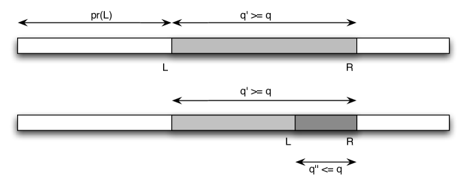
Updating : Assume that the left pointer is pointing at position , i.e. no unreported occurrence starts before . Notice that, if there is an occurrence of ending at any position , it must hold that . In other words, we must fit both and at position , so we update to
Updating : Assume that has just been updated. Thus, by definition of firstfit. If equality holds, then we have found an occurrence of in position , and can be incremented by . Otherwise , which implies that, interspersed between the characters that belong to , there are some “superfluous” characters. Now the first position where an occurrence of can start is at the beginning of a contiguous sequence of characters ending in which all belong to . In other words, we need the beginning of the longest suffix of with Parikh vector , i.e. the smallest position such that , or, equivalently, . Thus we update to
Finally, in order to check whether we have found an occurrence of query , after each update of or , we check whether . In Figure 2, we give the pseudocode of the algorithm.
- Algorithm Jumping Algorithm
-
Input:
query Parikh vector
-
Output:
A set containing all beginning positions of occurrences of in
-
1.
set ; ;
-
2.
while
-
3.
do ;
-
4.
if
-
5.
then add to ;
-
6.
;
-
7.
else;
-
8.
if
-
9.
then add to ;
-
10.
;
-
11.
return ;
It remains to see how to compute the firstfit and functions. We first prove that the algorithm is correct. For this, we will need the following lemma.
Lemma 2
The following algorithm invariants hold:
-
1.
After each update of , we have .
-
2.
After each update of , we have .
-
3.
.
Proof
1. follows directly from the definition of firstfit and the update rule for . For 2., if an occurrence was found at , then before the update we have and . Now is incremented by , so and , where is the ’th unity vector. Otherwise, , and again the claim follows directly from the definition of firstfit. For 3., if an occurrence was found, then is incremented by , and . Otherwise, . ∎
Theorem 4.1
Algorithm Jumping Algorithm is correct.
Proof
We have to show that (1) if the algorithm reports an occurrence, then it is correct, and (2) if there is an occurrence, then the algorithm will find it.
(1) If the algorithm reports an index , then is an occurrence of : An index is added to whenever . If the last update was that of , then we have by Lemma 2, and together with , this implies , thus is an occurrence of . If the last update was , then , and it follows analogously that .
(2) All occurrences of are reported: Let’s assume otherwise. Then there is a minimal and such that but is not reported by the algorithm. By Observation 1, we have .
Let’s refer to the values of and as two sequences and . So we have , and for all , and if and otherwise. In particular, for all .
First observe that if for some , , then will be updated to in the next step, and we are done. This is because . Similarly, if for some , , then we have .
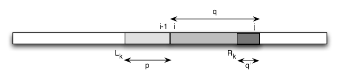
So there must be a such that . Now look at . Since there is an occurrence of after ending in , this implies that . However, we cannot have , so it follows that . On the other hand, by our assumption and by Lemma 2. So is pointing to a position somewhere between and , i.e. to a position within our occurrence of . Denote the remaining part of to the right of by : . Since , all characters of must fit between and , so the Parikh vector is a super-Parikh vector of . If , then there is an occurrence of at , and by minimality of , this occurrence was correctly identified by the algorithm. Thus, , contradicting our choice of . It follows that and we have to find the longest good suffix of the substring ending in for the next update of . But is a good suffix because its Parikh vector is a sub-Parikh vector of , so , again in contradiction to . ∎
We illustrate the proof in Fig. 3.
4.2 Variant using an inverted table
Storing all prefix vectors of would require storage space, which may be too much. Instead, we construct an “inverted prefix vector table” containing the increment positions of the prefix vectors: for each character , and each value up to , the position in of the ’th occurrence of character . Formally, for , and . Then we have
We can also compute the prefix vectors from table : For ,
The obvious way to find these values is to do binary search for in each row of . However, this would take time ; a better way is to use information already acquired during the run of the algorithm. By Lemma 2, it always holds that . Thus, for computing , it suffices to search for between and . This search takes time proportional to . Moreover, after each update of , we have , so when computing , we can restrict the search for to between and , in time . For more details, see Section 4.4.
Table can be computed in one pass over (where we take the liberty of identifying character with its index ). The variables count the number of occurrences of character seen so far, and are initialized to .
- Algorithm Construct
-
1.
for to
-
2.
;
-
3.
Table requires storage space (with constant 1). Moreover, the string can be discarded, so we have zero additional storage. (Access to is still possible, at cost .)
Example 2
Let and . The prefix vectors of are given below. Note that the algorithm does not actually compute these.
The inverted prefix table :
Query has 4 occurrences, beginning in positions , since . The values of and are given below:
| , see proof of Thm. 4.1 | 1 | 2 | 3 | 4 | 5 | 6 | 7 |
|---|---|---|---|---|---|---|---|
| L | 0 | 4 | 5 | 6 | 7 | 10 | 12 |
| R | 8 | 10 | 11 | 12 | 14 | 18 | 18 |
| occurrence found? | – | yes | yes | yes | – | – | yes |
4.3 Variant using a wavelet tree
A wavelet tree on allows rank, select, and access queries in time . For , , the number of occurrences of character up to and including position , while , the position of the ’th occurrence of character . When the string is clear, we just use and . Notice that
-
•
, and
-
•
for a Parikh vector , .
So we can use a wavelet tree of string to implement those two functions. We give a brief recap of wavelet trees, and then explain how to implement the two functions above in time each.
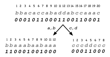
A wavelet tree is a complete binary tree with many leaves. To each inner node, a bitstring is associated which is defined recursively, starting from the root, in the following way. If , then there is nothing to do (in this case, we have reached a leaf). Else split the alphabet into two roughly equal parts, and . Now construct a bitstring of length from by replacing each occurrence of a character by if , and by if . Let be the subsequence of consisting only of characters from , and that consisting only of characters from . Now recurse on the left child with string and alphabet , and on the right child with and . An illustration is given in Fig. 4. At each inner node, in addition to the bitstring , we have a data structure of size , which allows to perform rank and select queries on bit vectors in constant time ([20, 9, 21]).
Now, using the wavelet tree of , any rank or select operation on takes time , which would yield time for both and . However, we can implement both in a way that they need only time: In order to compute , the wavelet tree, which has levels, has to be descended from the root to leaf . Since for , we need all values simultaneously, we traverse the complete tree in time.
For computing , we need , which can be computed bottom-up in the following way. We define a value for each node . If is a leaf, then corresponds to some character ; set . For an inner node , let be the bitstring at . We define by , where and are the values already computed for the left resp. right child of . The desired value is equal to .
Example 3
Let (cp. Fig. 4). We demonstrate the computation of using the wavelet tree. We have , where in slight abuse of notation we put the character in the subscript instead of its number. Denote the bottom left bitstring as , the bottom right one as , and the top bitstring as . Then we get , and . So at the next level, we compute .
4.4 Algorithm Analysis
Let denote the running time of the Jumping Algorithm using inverted tables over a text and a Parikh vector , and that of the Jumping Algorithm using a wavelet tree. Further, let be the number of iterations performed in the while loop in line 2, i.e., the number of jumps performed by the algorithm on the input
The time spent in each iteration depends on how the functions firstfit and are implemented (lines 3 and 7). In the wavelet tree implementation, as we saw before, both take time , so the overall runtime of the algorithm is
| (1) |
For the inverted table implementation, it is easy to see that computing firstfit takes time. Now denote, for each by the value of and after the ’th execution of line 3 of the algorithm, respectively.111The and coincide with the and from the proof of Theorem 4.1 almost but not completely: When an occurrence is found after the update of , then the corresponding pair is skipped here. The reason is that now we are only considering those updates that carry a computational cost. The computation of in line 3 takes : For each the component can be determined by binary search over the list By the claim follows.
The computation of in line 7 takes Simply observe that in the prefix ending at position there can be at most more occurrences of the ’th character than there are in the prefix ending at position Therefore, as before, we can determine by binary search over the list Using the fact that the desired bound follows.
The last three observations imply
Notice that this is an overestimate, since line 7 is only executed if no occurrence was found after the current update of (line 4). Standard algebraic manipulations using Jensen’s inequality (see, e.g. [16]) yield Therefore we obtain
| (2) |
4.4.1 Average case analysis of
The worst case running time of the Jumping Algorithm, in either implementation, is superlinear, since there exist strings of any length and Parikh vectors such that : For instance, on the string and , the algorithm will execute jumps.
This sharply contrasts with the experimental evaluation we present later. The Jumping Algorithm appears to have in practice a sublinear behavior. In the rest of this section we provide an average case analysis of the running time of the Jumping Algorithm leading to the conclusion that its expected running time is sublinear.
We assume that the string is given as a sequence of i.i.d. random variables uniformly distributed over the alphabet According to Knuth et al. [17] “It might be argued that the average case taken over random strings is of little interest, since a user rarely searches for a random string. However, this model is a reasonable approximation when we consider those pieces of text that do not contain the pattern […]”. The experimental results we provide will show that this is indeed the case.
Let us concentrate on the behaviour of the algorithm when scanning a (piece of the) string which does not contain a match. According to the above observation we can reasonably take this as a measure of the performance of the algorithm, considering that for any match found there is an additional step of size 1, which we can charge as the cost of the output.
Let denote the expected value of the distance between and , following an update of i.e. if is in position then we are interested in the value such that Notice that the probabilistic assumptions made on the string, together with the assumption of absence of matches, allows us to treat this value as independent of the position We will show the following result about For the sake of the clarity, we defer the proof of this technical fact to the next section.
Lemma 3
At each iteration (when there is no match) the pointer is moved forward to the farthest position from such that the Parikh vector of the substring between and is a sub-Parikh vector of In particular, we can upper bound the distance between the new positions of and with Thus for the expected number of jumps performed by the algorithm, measured as the average number of times we move , we have
| (3) |
Recalling (1) and (2), and using (3) for a random instance we have the following result concerning the average case complexity of the Jumping Algorithm.
Theorem 4.2
Let be fixed. Algorithm Jumping Algorithm finds all occurrences of a query
-
1.
in expected time using an inverted prefix table of size , which can be constructed in a preprocessing step in time ;
-
2.
in expected time using a wavelet tree of of size , which can be computed in a preprocessing step in time .
We conclude this section by remarking once more that the above estimate obtained by the approximating probabilistic automaton appears to be confirmed by the experiments.
4.4.2 The proof of Lemma 3
We shall argue asymptotically with and according to whether or not the Parikh vector is balanced, and in the latter case according to its degree of unbalancedness, measured as the magnitude of its largest and smallest components.
Case 1. is balanced, i.e., Then, from equations (7) and (12) of [19], it follows that
| (4) |
The author of [19] studied a variant of the well known coupon collector problem in which the collector has to accumulate a certain number of copies of each coupon. It should not be hard to see that by identifying the characters with the coupon types, the random string with the sequence of coupons obtained, and the query Parikh vector with the number of copies we require for each coupon type, the expected time when the collection is finished is the same as our It is easy to see that (4) provides the claimed bound of Lemma 3.
Case 2. Assume, w.l.o.g., that We shall argue by cases according to the magnitude of
Subcase 2.1. Suppose Let us consider again the analogy with the coupon collector who has to collect copies of coupons of type with Clearly the collection is not completed until the ’th copy of the coupon of type has been collected. We can model the collection of these type-1 coupons as a sequence of Bernoulli trials with probability of success The expected waiting time until the ’th success is and from the previous observation this is also a lower bound on Thus,
which confirms the bound claimed, also in this case.
Subcase 2.2. Finally, assume that Then, for the smallest component of we have Consider now the balanced Parikh vector We have that and By the analysis of Case 1., above, on balanced Parikh vectors, and observing that collecting implies collecting also, it follows that
in agreement with the bound claimed. This completes the proof.
4.5 Simulations
We implemented the Jumping Algorithm in C++ in order to study the number of jumps . We ran it on random strings of different lengths and over different alphabet sizes. The underlying probability model is an i.i.d. model with uniform distribution. We sampled random query vectors with length between () and , where is the length of the string. Our queries were of one of two types:
-
1.
Quasi-balanced Parikh vectors: Of the form with , and running from to . For simplicity, we fixed in all our experiments, and sampled uniformly at random from all quasi-balanced vectors around each .
-
2.
Random Parikh vectors with fixed length . These were sampled uniformly at random from the space of all Parikh vectors with length .
The rationale for using quasi-balanced queries is that those are clearly worst-case for the number of jumps , since depends on the shift length, which in turn depends on . Since we are searching in a random string with uniform character distribution, we can expect to have minimal if is close to balanced, i.e. if all entries are roughly the same. This is confirmed by our experimental results which show that decreases dramatically if the queries are not balanced (Fig. 7, right).
We ran experiments on random strings over different alphabet sizes, and observe that our average case analysis agrees well with the simulation results for random strings and random quasi-balanced query vectors. Plots for and with alphabet sizes resp. are shown in Fig. 6.
In Fig. 5 we show comparisons between the running time of the Jumping algorithm and that of the simple window algorithm. The simulations over random strings and Parikh vectors of different sizes appear to perfectly agree with the guarantees provided by our asymptotic analyses. This is of particular importance from the point of view of the applications, as it shows that the complexity analysis does not hide big constants.


To see how our algorithm behaves on non-random strings, we downloaded human DNA sequences from GenBank [12] and ran the Jumping Algorithm with random quasi-balanced queries on them. We found that the algorithm performs 2 to 10 times fewer jumps on these DNA strings than on random strings of the same length, with the gain increasing as increases. We show the results on a DNA sequence of million bp (from Chromosome 11) in comparison with the average over 10 random strings of the same length (Fig. 7, left).


5 Conclusion
Our simulations appear to confirm that in practice the performance of the Jumping Algorithm is well predicted by the average case analysis we proposed. A more precise analysis is needed, however. Our approach seems unlikely to lead to any refined average case analysis since that would imply improved results for the intricate variant of the coupon collector problem of [19].
Moreover, in order to better simulate DNA or other biological data, random string models other than uniform i.i.d. should also be analysed, such as first or higher order Markov chains.
We remark that our wavelet tree variant of the Jumping Algorithm, which uses rank/select operations only, opens a new perspective on the study of Parikh vector matching. We have made another family of approximate pattern matching problems accessible to the use of self-indexing data structures [21]. We are particularly interested in compressed data structures which allow fast execution of rank and select operations, while at the same time using reduced storage space for the text. Thus, every step forward in this very active area can provide improvements for our problem.
Acknowledgements
We thank Gonzalo Navarro for fruitful discussions.
References
- [1] A. Amir, A. Apostolico, G. M. Landau, and G. Satta. Efficient text fingerprinting via Parikh mapping. J. Discrete Algorithms, 1(5-6):409–421, 2003.
- [2] A. Apostolico and R. Giancarlo. The Boyer-Moore-Galil string searching strategies revisited. SIAM J. Comput., 15(1):98–105, 1986.
- [3] G. Benson. Composition alignment. In Proc. of the 3rd International Workshop on Algorithms in Bioinformatics (WABI’03), pages 447–461, 2003.
- [4] S. Böcker. Sequencing from compomers: Using mass spectrometry for DNA de novo sequencing of 200+ nt. Journal of Computational Biology, 11(6):1110–1134, 2004.
- [5] S. Böcker. Simulating multiplexed SNP discovery rates using base-specific cleavage and mass spectrometry. Bioinformatics, 23(2):5–12, 2007.
- [6] R. S. Boyer and J. S. Moore. A fast string searching algorithm. Commun. ACM, 20(10):762–772, 1977.
- [7] A. Butman, R. Eres, and G. M. Landau. Scaled and permuted string matching. Inf. Process. Lett., 92(6):293–297, 2004.
- [8] M. Cieliebak, T. Erlebach, Zs. Lipták, J. Stoye, and E. Welzl. Algorithmic complexity of protein identification: combinatorics of weighted strings. Discrete Applied Mathematics, 137(1):27–46, 2004.
- [9] D. Clark. Compact pat trees. PhD thesis, University of Waterloo, Canada, 1996.
- [10] R. Eres, G. M. Landau, and L. Parida. Permutation pattern discovery in biosequences. Journal of Computational Biology, 11(6):1050–1060, 2004.
- [11] W. Feller. An Introduction to Probability Theory and Its Applications. Wiley, 1968.
- [12] Website. http://www.ncbi.nlm.nih.gov/Genbank/.
- [13] R. Grossi, A. Gupta, and J. S. Vitter. High-order entropy-compressed text indexes. In SODA, pages 841–850, 2003.
- [14] R. N. Horspool. Practical fast searching in strings. Softw., Pract. Exper., 10(6):501–506, 1980.
- [15] P. Jokinen, J. Tarhio, and E. Ukkonen. A comparison of approximate string matching algorithms. Software Practice and Experience, 26(12):1439–1458, 1996.
- [16] S. Jukna. Extremal Combinatorics. Springer, 1998.
- [17] D. E. Knuth, J. H. Morris Jr., and V. R. Pratt. Fast pattern matching in strings. SIAM J. Comput., 6(2):323–350, 1977.
- [18] M. Lothaire. Applied Combinatorics on Words (Encyclopedia of Mathematics and its Applications). Cambridge University Press, New York, NY, USA, 2005.
- [19] R. May. Coupon collecting with quotas. Electr. J. Comb., 15, 2008.
- [20] J. I. Munro. Tables. In Proc. of Foundations of Software Technology and Theoretical Computer Science (FSTTCS’96), pages 37–42, 1996.
- [21] G. Navarro and V. Mäkinen. Compressed full-text indexes. ACM Comput. Surv., 39(1), 2007.
- [22] A. Salomaa. Counting (scattered) subwords. Bulletin of the European Association for Theoretical Computer Science (EATCS), 81:165–179, 2003.
- [23] W. F. Smyth. Computing Patterns in Strings. Pearson Addison Wesley (UK), 2003.