Algorithms for Maximum Internal Spanning Tree Problem for Some Graph Classes 111The third author is supported by an NSF Graduate Research Fellowship under Grant No. DGE-1650044.
Abstract
For a given graph , a maximum internal spanning tree of is a spanning tree of with maximum number of internal vertices. The Maximum Internal Spanning Tree (MIST) problem is to find a maximum internal spanning tree of the given graph. The MIST problem is a generalization of the Hamiltonian path problem. Since the Hamiltonian path problem is NP-hard, even for bipartite and chordal graphs, two important subclasses of graphs, the MIST problem also remains NP-hard for these graph classes. In this paper, we propose linear-time algorithms to compute a maximum internal spanning tree of cographs, block graphs, cactus graphs, chain graphs and bipartite permutation graphs. The optimal path cover problem, which asks to find a path cover of the given graph with maximum number of edges, is also a well studied problem. In this paper, we also study the relationship between the number of internal vertices in maximum internal spanning tree and number of edges in optimal path cover for the special graph classes mentioned above.
1 Introduction
The Maximum Internal Spanning Tree (MIST) problem is a degree based spanning tree optimization problem, in which we ask to find a spanning tree of a given graph such that the number of vertices of degree at least two is maximized. The MIST problem is motivated by telecommunication network design [22]. We also believe that MIST problem has its own theoretical importance as it is a generalization of the Hamiltonian path problem, a known NP-complete problem [5]. The Hamiltonian path problem remains NP-complete for chordal graphs and chordal bipartite graphs [10, 18]. Hence, we also do not expect polynomial time algorithms for the MIST problem in chordal graphs and chordal bipartite graphs.
The dual problem to MIST, the Minimum Leaves Spanning Tree (MLST) problem asks to find a spanning tree with minimum number of leaves for a given graph. The MLST problem cannot be approximated within any constant factor unless P=NP [17]. Unlike MLST, several constant factor approximation algorithms have been proposed for the MIST problem in literature. In , Prieto et al. [20] gave a -approximation algorithm for the MIST problem whose running time was later improved by Salamon et al. in 2008 [23]. Salamon also gave approximation algorithms for claw-free and cubic graphs with approximation factors and respectively [23]. In 2009, Salamon [21] gave a -approximation algorithm for graphs with no pendant vertices and later, in 2015, Knauer et al. [9] showed that a simplified and faster version of Salamon’s algorithm yields a -approximation algorithm even on general graphs. In 2014, Li et al. proposed a -approximation algorithm using a different approach for general undirected graphs and improved this ratio to for graphs without leaves [14]. Li et al. gave a -approximation algorithm for general graphs using depth-5 local search [13]. In 2018, Chen et al. presented a -approximation algorithm which is the best approximation factor till now [2]. Several FPT-algorithms have also been designed for the MIST problem where the considered parameter is the solution size [20, 13, 3, 4, 1, 12].
For finding efficient algorithms for the MIST problem, it is often useful to reduce the MIST problem to the path cover problem. A path cover of a graph is a spanning subgraph such that every component of is a path. A path cover with maximum number of edges is called an optimal path cover of . If denotes an optimal path cover of a graph, then number of edges in is denoted by . In 2018, Li et al. proposed a polynomial time algorithm for the MIST problem in interval graphs [15]. They also proved that number of internal vertices in any MIST of any graph is at most , where is an optimal path cover of . We will observe that number of internal vertices in any MIST of a chain graph is either or and is for cographs. For bipartite permutation, block and cactus graphs, we prove that there is no constant such that is the lower bound on the number of internal vertices in any MIST of such graphs. We also propose linear-time algorithms for the MIST problem in bipartite permutation graphs, block graphs, cactus graphs and cographs. A hierarchy relationship between these classes of graphs is shown in Fig. 1.
The structure of the paper is as follows. In Section 2, we give some basic definitions and notations used in the paper. In Section 3, we discuss MIST problem for block graphs and cactus graphs and provide linear-time algorithms for both these graph classes. In Section 4, we prove that MIST of cographs can be computed in linear-time by providing an algorithm. In Section 5, we present a linear-time algorithm to find a MIST of an arbitrary bipartite permutation graph. In Section 6, we prove a bound for chain graphs regarding number of internal vertices in its MIST. Finally, Section 7 concludes the paper.

2 Preliminaries
Let be a graph. In this paper, we only consider simple, undirected and connected graphs. For a vertex denotes the degree of in and denotes the neighborhood of in . When there is no ambiguity regarding the graph , we simply use and , to represent the degree of and neighborhood of , respectively. A vertex in is called pendant if . The set of pendant vertices in is denoted by . The vertex adjacent to a pendant vertex is called the support vertex of , and is denoted by . A vertex is called internal, if is not pendant, that is, . Let denotes the set of internal vertices in , and . For a set and a spanning tree of , we define .
For vertices and , we denote an edge between and by . For a subset of , denotes the subgraph of obtained after removing vertices of and edges incident on these vertices from . If , then we simply write for . A vertex of a graph is called a cut vertex if is disconnected.
Throughout this paper, denotes the number of vertices and denotes the number of edges in . A graph is said to be bipartite if can be partitioned into two disjoint sets and such that every edge of joins a vertex in to a vertex in . Such a partition of is called a bipartition. A bipartite graph with bipartition of is denoted by . For a set , an induced subgraph is the graph whose vertex set is and edge set consists of all the edges in that have both the endpoints in , and is denoted by . If , is a complete subgraph of , then is called a clique of .
A subgraph of is called a spanning subgraph if it contains all the vertices of . A path cover of a graph is a spanning subgraph such that every component of is a path. A path cover is an optimal path cover if it has the maximum number of edges. A spanning subgraph of which is also a tree is called a spanning tree of . A spanning tree is called a maximum internal spanning tree(MIST) if it contains the maximum number of internal vertices among all the spanning trees of . For a graph , the number of internal vertices in any MIST of is denoted by .
Now we state a useful theorem which gives an upper bound on the number of internal vertices in a MIST with respect to the graph’s optimal path cover.
Theorem 2.1.
[15] For a graph , the number of internal vertices in a maximum internal spanning tree of is less than the number of edges in an optimal path cover of , that is, , where denotes an optimal path cover of . Moreover, this bound is tight.
Note that the vertices which are pendant in itself, will be pendant in any MIST of . Hence, we have the following observation.
Observation 2.1.
For a graph , if is a pendant vertex and is the support vertex of in , then remains a pendant vertex and remains adjacent support vertex of in any MIST of .
Suppose is not a tree and is adjacent to pendant vertices, say . Let . Then based on above observation, the number of internal vertices in a MIST of will be same as the number of internal vertices in any MIST of . It is also easy to obtain a MIST of from any MIST of . Hence, throughout this work, we assume that every vertex has at most one pendant vertex adjacent with it.
Below, we give another result regarding the number of pendant vertices in a spanning tree of a bipartite graph. Note that, if we have number of internal vertices in a spanning tree of from one partite set, then at least vertices must be present in the neighborhood of these vertices, which lie in the other partite set of the bipartite graph .
Observation 2.2.
Let be a bipartite graph with . If , then there are at least pendant vertices from in any spanning tree of . Similarly, if , then there are at least pendant vertices from in any spanning tree of .
3 Block and Cactus Graphs
In this section, we discuss the MIST problem for block graphs and cactus graphs. We will show that the MIST problem can be solved in linear-time for both classes of graphs. Block and cactus graphs will also provide our first family of examples in which cannot be lower bounded in terms of where is an optimal path cover of and is some constant.
A block of a graph is a maximal connected subgraph with no cut vertices. Note that a block of is either an edge or a 2-connected subgraph. The set of blocks of a graph is called the block decomposition of and is denoted by . Let and be two vertices belonging to , then a path between and , which contains all the vertices of the block , is called a spanning path between and in . We say a block is good if there exists distinct such that both and are cut vertices of and has a spanning path between and . A block is said to be bad otherwise. Let denote the set of bad blocks of .
A block graph is a graph in which every block is a clique. If a block graph contains only one block then is a complete graph. A block graph is said to be nontrivial if it contains at least two blocks. Note that a trivial block has a Hamiltonian path. Thus for the remainder of the section we only consider nontrivial block graphs.
Let be a nontrivial block graph. Bad blocks of have another characterization which we state as the Observation 3.1.
Observation 3.1.
A block of a block graph is bad if and only if it contains exactly one cut vertex of .
A graph is a cactus graph if every block of is either a cycle or an edge. If a cactus graph contains only one block then is either a cycle or an edge and in that case finding a MIST of is trivial. Again, a cactus graph is said to be nontrivial if it contains at least two blocks and now we only consider nontrivial cactus graphs.
Let be a nontrivial cactus graph. A block of is called an end block of if it contains exactly one cut vertex of . Note that an end block of a cactus graph is also a bad block of . Bad blocks of a cactus graph have another characterization which we state in the following observation.
Observation 3.2.
A block of a cactus graph is bad if and only if does not contain two adjacent cut vertices of .
If and are two blocks of a block/cactus graph and , then and the vertex is a cut vertex of . Let be a MIST of a nontrivial block/cactus graph . Below, we state two observations which hold true for both block and cactus graphs.
Observation 3.3.
must have at least one leaf in every bad block of .
Observation 3.4.
, where denotes the number of internal vertices in .
Recall that block decomposition of a graph is the set of blocks of . It can be computed in time using the following approach. Let be a cut vertex of a block/cactus graph and be the connected components of the graph . Let denotes the subgraph , for each . We call the -components of . The block decomposition of a block/cactus graph can be found by recursively choosing a cut vertex and computing the -components.
3.1 Algorithm for Block and Cactus Graphs
In this subsection, we first prove a theorem which relates the number of internal vertices in a MIST of a block/cactus graph to the number of bad components of . Then, we outline a linear-time algorithm to compute a MIST of .
Theorem 3.1.
Let be a graph with a nontrivial block decomposition such that each block has a spanning path with a cut vertex as an endpoint. Then has a spanning tree in which number of internal vertices is .
Proof.
Let be the number of blocks in and be an arbitrary block of . If is good, then let be a spanning path between two cut vertices of . If is bad, we let be a spanning path with a single cut vertex as an endpoint. Let . Note that is a spanning tree of . Furthermore, as any cut vertex of cannot be a leaf of , we have . ∎
The proof of Theorem 3.1 gives a simple algorithm for a block or cactus graph. First find a block decomposition, this takes time. Then for each block , determine if is bad or not and find the corresponding path. This takes time. In total we have a linear-time algorithm. As both block and cactus graphs satisfy the hypothesis of Theorem 3.1, combining with Obervation 3.4 we have the following,
Corollary 3.1.
If is a block or cactus graph, then .
3.2 Relationship between and
We now show for a block or cactus graph there does not exist a constant such that where is an optimal path cover of . Recall Corollary 3.1 states that and Theorem 2.1 states . Note that the number of edges in the optimal path cover and the number of components in adds up to . So, we see that . Thus, for both block and cactus graphs.
For every integer , we construct a connected graph with vertices and . The graph is both a block graph and a cactus graph as every block of is either an edge or a clique on three vertices. The vertex set of is , where for each . The edge set is , where for each and contains the edges of the form for . Note . We obtain an optimal path cover for having edges and components [19]. The number of bad blocks in is . Using Theorem 3.1, we obtain a MIST of with internal vertices. Thus, . Fig. 2 provides an illustration for .

Here, we see that which implies that for arbitrary , we have . So, block and cactus graphs do not have lower bound for of the form for some fixed natural number , independent of .
4 Cographs
In this section, we discuss the MIST problem for cographs. The complement-reducible graphs or cographs have been discovered independently by several authors since the 1970s [24, 8]. In the literature, the cographs are also known as -free graphs, -graphs, Hereditary Dacey graphs and -parity graphs. The class of cographs is defined recursively as follows:
-
•
A single-vertex graph is a cograph;
-
•
If is a cograph, then its complement is also a cograph;
-
•
If and are cographs, then their disjoint union is also a cograph.
Cographs admit a rooted tree representation. This tree is called cotree of a cograph , denoted . The cotree of a cograph rooted at a node possesses the following properties.
-
1.
Every internal vertex except has at least two children. Furthermore, has exactly one child if and only if the underlying cograph is disconnected.
-
2.
The internal nodes are labeled by either (-nodes) or (-nodes) in such a way that the root is always a -node, and -nodes and -nodes alternate along every path in starting at the root.
-
3.
The leaves of are precisely the vertices of , such that vertices and are adjacent in if, and only if, the lowest common ancestor of and in is a -node.
Fig. 3 illustrates a cograph along with its cotree .

According to [16], the cotree of any cograph can be preprocessed such that it is a binary tree. So, we may assume that is a binary tree rooted at a vertex . The set of leaves of the left subtree of is denoted by and the set of leaves of the right subtree of is denoted by .
Note that every leaf of represents a vertex of the graph . If we consider one vertex from and one vertex from then their least common ancestor is the root node. As the root node is always a -node, we have the following observation.
Observation 4.1.
For any , we have .
Recall that a path cover of a graph is a spanning subgraph such that every component of is a path. A path cover is an optimal path cover if it has the maximum number of edges. [16] gave a linear-time algorithm to compute an optimal path cover of a cograph . The optimal path cover constructed in [16] is one of the following type:
-
•
The path cover contains a single path component which is a Hamiltonian path of .
-
•
The path cover contains at least two path components. In this case, there exists exactly one path in which contains vertices from both the sets and and all other paths in contain vertices from only. Fig. 4 illustrates this case.

Note that by Theorem 2.1 we have for an optimal path cover . Below, we give a theorem which implies that Algorithm 1 also outputs a spanning tree which attains this upper bound.
Theorem 4.1.
Algorithm 1 outputs a spanning tree of a cograph such that, , where is an optimal path cover of . Hence, .
Proof.
Let be the optimal path cover computed in step 1 of Algorithm 1. If , then has a Hamiltonian path and Algorithm 1 returns a Hamiltonian path. Now, suppose , then the path contains vertices from both sets and and for all . Now, let such that is not an end vertex of .
For each path in , consider a pendent vertex of the path. By Observation 4.1, and are adjacent. Let . These new edges connect one internal vertex with a pendant vertex of path of . This is illustrated by the dash edges in Fig. 4. Note then the number of internal vertices of is , hence by Theorem 2.1. ∎
5 Bipartite Permutation Graphs
In this section, we discuss the MIST problem for bipartite permutation graphs. A graph with is said to be a permutation graph if there is a permutation over such that if and only if . Intuitively, each vertex in a permutation graph corresponds to a line segment joining two points on two parallel lines and , which is called a line representation. Then, two vertices and are adjacent if and only if the corresponding line segments and are crossing. Vertex indices give the ordering of the points on , and the permutation of the indices gives the ordering of the points on . When a permutation graph is bipartite, it is said to be a bipartite permutation graph.
A strong ordering of a bipartite graph consists of an ordering of and an ordering of , such that for all edges with and : if and then and are edges in . An ordering of has the adjacency property if, for every vertex in , its neighbors in are consecutive in . The ordering has the enclosure property if, for every pair of vertices of with , the vertices of appear consecutively in . These properties are useful for characterizing bipartite permutation graphs.
[7] proved that a bipartite graph is a bipartite permutation graph if and only if it admits a strong ordering. Furthermore if we assume that the graph is connected, then we can say more.
Lemma 5.1.
[7] Let be a strong ordering of a connected bipartite permutation graph . Then both and have the adjacency property and the enclosure property.
Throughout this section, denotes a connected bipartite permutation graph. A strong ordering of a bipartite permutation graph can be computed in linear-time [25]. Let be a strong ordering of , where and . We write strong ordering of vertices of as . For , we write if and appears before in the strong ordering; we define in a similar manner. We write (or, ) when . For vertices of , denotes either , , or holds.
Since each vertex of satisfies the adjacency property, the neighborhood of any vertex consists of consecutive vertices in the strong ordering. We define the first neighbor of a vertex as the vertex with minimum index in its neighborhood and the last neighbor of a vertex as the vertex with maximum index in its neighborhood. We notate the first and last neighbors of a vertex as and respectively. Combining the above statements for a bipartite permutation graph with its strong ordering , has the following properties [11]:
-
1.
For any vertex of , its neighborhood consists of consecutive vertices in or .
-
2.
For any pair of vertices from or , if then and .
Now, we define some terminology which we require for the remainder of this section. A vertex with is of type 1 if . A vertex with is of type 1 if . Similarly, a vertex with is of type 2 if and a vertex with is of type 2 if . Note that a type 2 vertex is also a type 1 vertex but the converse may not be true. Furthermore, a type 1 vertex is also a type 2 vertex. Characterizing the vertices in this way is an important distinction for our algorithm. We now prove two important lemmas which will be used to prove the correctness of Algorithm 2.
Lemma 5.2.
Let . Furthermore, suppose each vertex of and is of type 1 except , and . Then there exists a MIST of , in which are are pendant. Moreover; if , then the support vertex of is of degree at least in .
Proof.
We first show for all . Suppose there exists such that . Let and . As both and are type 1, we have and . As is a strong ordering, we have , a contradiction. Thus we may assume . Furthermore as is type 1, we have for all .
Suppose . Note that as is a strong ordering of , we have for all , . As we assumed is connected, we have that as well. Note that this implies that has the Hamiltonian path which is a MIST. So, we may assume that .
Now, let be a MIST of . If and are pendant in and degree of is at least in , then we are done. Suppose otherwise, and we modify in the following way. We first remove all edges of incident with the vertices of and then add edges to obtain a new graph . Note that as , is connected.
First suppose contains no cycle. Note that is a spanning tree of . If , then as we can choose an edge in such that . Since the strong ordering of the vertices of satisfies property , we have . So we can further modify by removing the edge and replacing with the edge We see that
So, we have . Since is a spanning tree and is a MIST of , we have that is also a MIST. Thus, we obtain our desired MIST in which are are pendant and the support vertex of is of degree at least .
Now, suppose contains a cycle . This implies that there exists such that with . Now, we modify by removing the edge . This step reduces degree of by while leaving the graph connected. We repeat this modification until has no more cycles, thus will be a spanning tree of . Let us assume that there are such vertices which became pendant in this process of updating . Let be the set of vertices. Note these vertices were internal in . Suppose . As , then the subforest of induced by the set would have at least edges. As , this contradicts the fact that was a tree. Thus we have . It follows,
Again, we have which implies that is also a MIST. If , then we can choose an edge in , such that . Since the strong ordering satisfies property , we have . So we update the tree by removing the edge and adding the edge . Thus, we obtain a MIST in which are are pendant and support vertex of is of degree at least . ∎
Lemma 5.3.
Let . Furthermore, suppose each vertex of and is of type 1 except , and .
-
(a)
If for all , then there exists a MIST of , in which is pendant.
-
(b)
If there exists , then there exists a MIST of , in which and are pendant. Moreover; if , then support vertex of is of degree at least in .
Proof.
We first argue that for . First assume for some , . As both and are type 1, we have and . As is a strong ordering, we have , a contradiction. Furthermore, as is type 1, we have for all .
Suppose . As , and is connected we have that as well. Note then if for all , then is a Hamiltonian path. Otherwise, if there exists , then the path and gives the desired Hamiltonian path.
So, we may assume that and we will first prove part (a). Let be a MIST of and suppose is not pendant in . Let be the graph obtained from where we remove all edges incident to the vertices of and add edges . Note as , is pendant in .
First, suppose contains no cycles. Note then that is a spanning tree of . We argue that we may assume . Suppose otherwise, that is, . Let such that . As the strong ordering of the vertices of satisfies property 2, we have as well. So we further modify by removing the edge and adding the edge . We see that
So, we have that . Since is a spanning tree and is a MIST of , is also a MIST of .
Next, suppose is not a tree. We now modify to remove the cycles. Let be a cycle of . Note then there is a vertex such that with . We then modify by removing the edge . Note that the degree of decreases by 1. We repeat this process until no cycles remain in . Assume that cycles were removed during this process and thus at most pendant vertices were created in this process. As and is a tree, we have . We see that,
Again, we have that which implies that is also a MIST. Hence, part (a) holds.
Next, we prove part (b). Let be a MIST of . If and are pendant in and degree of is at least in , then we are done, so assume otherwise. Let be the graph obtained from modifying where we remove all edges incident on the vertices of and add edges and .
First suppose contains no cycle, then is a spanning tree of . If , then we are done modifying, so suppose . As and , there exists an edge in . Since the strong ordering of the vertices of satisfies property 2, we have . Thus we further modify where we remove and add the edge . As we assumed there exists a such that , we have . Let and note . By Observation 2.2, we see that for any spanning tree of , contains at least one pendant vertex. So, .We see that
Again, we have which implies that is a MIST. Thus, we obtained a MIST in which and are pendant and support vertex of is of degree at least .
Now, suppose contains a cycle. We now modify to be a spanning tree. Let be a cycle contained in . This implies that there is a vertex such that with . We remove the edge from . This decreases the degree of by 1. We repeat this process until no cycles remain in . Let with be the set of the vertices made pendant in this process. Suppose . As , the subgraph of induced by has at least edges. As , this contradicts the fact that is a tree. Thus we may assume . As before, we may assume . It follows,
This implies that is also a MIST. Thus, we obtained a MIST in which and are pendant and support vertex of is of degree at least . ∎
We state similar results when the vertices are of type . By symmetry, the proofs of Lemmas 5.4 and 5.5 follow from Lemmas 5.2 and 5.3.
Lemma 5.4.
Let . Furthermore, suppose each vertex of and is of type 2 except , and . Then there exists a MIST of , in which are are pendant. Moreover; if , then support vertex of is of degree at least in .
Lemma 5.5.
Let . Furthermore, suppose each vertex of and is of type 2 except , and .
-
(a)
If , then there exists a MIST of , in which is pendant.
-
(b)
If , then there exists a MIST of , in which and are pendant. Moreover; if , then support vertex of is of degree at least in .
Next, we propose an algorithm to find a MIST of based on the Lemmas 5.2, 5.3, 5.4 and 5.5. In our algorithm, we first find a vertex such that it is a pendant vertex in some MIST of and the degree of support vertex of in is at least . Now, if we remove from and call the remaining graph , then we see that the number of internal vertices in a MIST of is same as the number of internal vertices in a MIST of . Note that we can easily construct a MIST of from a MIST of by adding the pendant vertex to the corresponding support vertex. So, after finding the vertex , the problem is reduced to finding MIST of , say . We continue doing the same until no such vertex exists and then the resultant graph has a Hamiltonian path.
In our algorithm, we visit the vertices alternatively from the partitions and . We consider two special orderings and of which we call and , respectively. Below, we describe the method to find a vertex which is pendant in some MIST of and is at least .
We first visit the vertices of in the ordering and search for the first vertex, which is not of type 1. Let be such a vertex. If or and the conditions of part (b) of Lemma 5.3 are satisfied, then there exists a MIST of in which is a pendant vertex and the degree of support vertex of in is at least . So, we remove from and find a MIST of . Later, we obtain a MIST of by adding to . But, if , say and conditions of part (a) of Lemma 5.3 are satisfied, then there exists a MIST of in which is a pendant vertex. In this case, we start visiting the vertices of in the ordering , starting from . At this step, we do not maintain any information from search.
Now, let be the first vertex not of type 2 in the ordering . If or and the conditions of part (b) of Lemma 5.5 are satisfied, then there exists a MIST of in which is a pendant vertex and the degree of support vertex of in is at least . So, we remove from and find a MIST of . Later, we obtain a MIST of by adding to . Here, if and conditions of part (a) of Lemma 5.5 are satisfied, then there exists a MIST of in which is a pendant vertex. But, we have already explored this possibility while visiting the vertices of in the ordering . So, we do not get such a vertex . To see this, suppose that we get such a vertex . Then, for some , where . Now, part (a) of Lemma 5.5 tells that for all implying that . But, while visiting the vertices in the ordering , we got a vertex satisfying , so , a contradiction.
The detailed procedure for computing a MIST of a bipartite permutation graph is presented in Algorithm 2. Algorithm 2 either finds a vertex which is not of type 1 or a vertex which is not of type 2. When such a vertex is found, we call as an encountered vertex. All the encountered vertices are found while executing the steps written in lines 4, 11, 17, 22, 31 or 39 of Algorithm 2. We see that the algorithm returns a spanning tree of . Before proving the correctness of the Algorithm 2, we state a necessary lemma.
Lemma 5.6.
Let be the input bipartite permutation graph for the Algorithm 2 and denotes the first encountered vertex in either the or search. Suppose that is the spanning tree of returned by Algorithm 2. Let be the set of vertices which are visited from side till and be the set of vertices which are visited from side till . Then there exists a MIST of such that .
Proof.
We have four cases to consider.
Case 1: and it is not of type 1. Then the vertex was found when flag = 1 in Algorithm 2, that is, when searching for the first vertex not of type 1. Let for some . Then the sets satisfy the hypothesis of Lemma 5.2. Thus by Lemma 5.2, there exists a MIST of such that . In particular, .
Now, we prove the correctness of Algorithm 2.
Theorem 5.1.
Algorithm 2 returns a maximum internal spanning tree of .
Proof.
Let be a MIST of and be the spanning tree of returned by Algorithm 2. Recall in the execution of Algorithm 2, we either search for a vertex not of type 1 with the ordering or we search for a vertex not of type 2 with the ordering . This is ensured since either we never arrive at line 17 or we arrive at it once and after that flag remains 2 throughout the algorithm. Let be the sequence of vertices encountered in the execution of Algorithm 2. Let and denote the set of vertices visited till from and side respectively. For , let denotes the set of vertices visited from side after and upto . Similarly, let denotes the set of vertices visited from side after and upto . Let and denote the set of all vertices visited after from and side respectively.
First suppose Algorithm 2 is searching for a vertex not of type 1 with the ordering and it never arrives at line 17. This means that flag is 1 throughout the algorithm. To prove that is a MIST of , we will prove that can be modified so that it remains a MIST of and is same as , that is,
| (1) |
We prove (1) using induction on . If , we have due to Lemma 5.6. Hence, (1) is true for . Assume that (1) is true for .
We now show that (1) is true for . So, consider vertex for . Two possible cases arise.
Case 1: .
First suppose for every . Then for and , we have and . As by Observation 2.2 we have that the number of pendant vertices from in any spanning tree of is at least . Therefore .
If , we remove all edges of who have one end in and the other in and all edges incident with the vertices of within . We then add all edges from and the edge of which connects to in . If cycles were created in this process, then we can remove those cycles without introducing more pendant vertices using the method discussed in Lemmas 5.2 and 5.3. Let denote this updated tree. We have,
Thus is also a MIST of such that
Now, suppose for some . We choose the largest such that . Then for and , we have and . As , by Observation 2.2 we have that the number of pendant vertices from in any spanning tree of is at least . Therefore, .
If , we remove all edges of whose one end belongs to and another end to , all edges incident on the vertices of from and add all edges from and the edge of which connects to in . If cycles were created in this process, then we can remove those cycles without introducing more pendant vertices using the method discussed in Lemmas 5.2 and 5.3. So, we may assume these modifications of do not create any cycles. Let denotes the updated tree. We have,
Thus, is also a MIST of such that
Case 2: .
First suppose for every . Then for and , we have and . As by Observation 2.2 we have that the number of pendant vertices from in any spanning tree of is at least . Therefore . Here, , so, let for some . As we have assumed that flag is 1, this implies that there exists an index such that . So, for and , we have . Now, by Observation 2.2, we know that the number of pendant vertices within in any spanning tree of is at least . So, , implying that .
If , we remove all edges of who have one end in and the other in and all edges incident with the vertices of within . We then add all edges from and the edge of which connects to in . As before, if cycles are present, we may further modify to remove these cycles without introducing more pendant vertices. Let denote this updated tree. We have,
Thus is also a MIST of such that
Now, suppose there is some vertex of side among the vertices for . We choose the largest such that . Then for and , we have and . As , by Observation 2.2 we have that the number of pendant vertices from in any spanning tree of is at least . Therefore, .
If , we remove all edges of who have one end in and the other in and all edges incident with the vertices of within . We then add all edges from and the edge of which connects to in . As before, if we created cycles with this modification, we remove them with the same method used in Lemmas 5.2 and 5.3. Let denote this updated tree. We have,
Thus is also a MIST of such that
If algorithm arrives at line 17, then flag changes to 2 and it remains 2 throughout the algorithm. So, it searches vertex not of type 2 in the ordering starting from . There will be analogous arguments for this case also, using Lemmas 5.4 and 5.5 instead. For a quick justification why, with the assumption flag = 1, the above analysis fails if we encounter a vertex, say , such that is not type 1 and for all . The analogous failure case for the flag = 2 is, when we encounter a vertex that is not of type 2 and for all . Note that these cases cannot simultaneously occur. Otherwise the analysis is symmetric. Consequently, Algorithm 2 returns a maximum internal spanning tree of . ∎
Now, we discuss the running time of Algorithm 2. Suppose Algorithm 2 returns a MIST . Recall that we visit the vertices in one of the orders , or . Furthermore, any vertex encountered during the execution of the algorithm must be pendant in . As we never visit the same vertex twice, these pendant vertices are found in linear-time. The remaining graph must have a Hamiltonian path, and finding the Hamiltonian path is also linear-time in our algorithm. So, all the steps of Algorithm 2 can be executed in time. Hence we have the following corollary.
Corollary 5.1.
A maximum internal spanning tree of a bipartite permutation graph can be computed in linear-time.
6 Bounds for Chain Graphs
A bipartite graph is a chain graph if the neighborhoods of the vertices of form a chain, that is, the vertices of can be linearly ordered, say such that and . If is a chain graph, then the neighborhoods of the vertices of also form a chain. If , an ordering is called a chain ordering if and . If a vertex appears before in chain ordering, we write . Given a chain graph , a chain ordering of can be computed in linear-time [6]. Note that a chain ordering is also a strong ordering. So, every chain graph is also bipartite permutation graph.
In this section, we will prove the following lower bound for number of internal vertices in a MIST of a chain graph G.
Theorem 6.1.
For a chain graph , let be an optimal path cover of . Then .
In order to prove Theorem 6.1, we look at optimal path covers of bipartite permutation graphs. [26] gave an algorithm to find an optimal path cover of a bipartite permutation graph. Note that this algorithm applies to chain graphs as well. We will recall the algorithm given in [26], but first we cover some notations used in the algorithm. A path cover is contiguous if it satisfies the following two conditions:
-
1.
If is the only vertex in and if , then and belong to different paths.
-
2.
If is an edge in and is an edge in , where and , then .
A path is contiguous if it is one of the following forms: , , , or such that and . Note that every path in a contiguous path cover is contiguous. Let be a contiguous path which ends with some edge, say . If , then we say that the path is not extendable on the right. A contiguous path is said to be a maximal contiguous path if it is not extendable on the right. An optimal path cover is a maximum optimal path cover if each covers the maximum number of vertices in According to [26], there exists an optimal path cover which is a maximum optimal path cover for any bipartite permutation graph such that every path in the path cover is a maximal contiguous path.
As a chain graph is an instance of a bipartite permutation graph, we recall the algorithm from [26] which finds this desired maximum optimal path cover for a chain graph (Algorithm 3). From this point, we will refer such a path cover as an optimal path cover only.
Now, we give the proof of Theorem 6.1.
Proof of Theorem 6.1.
Let be the optimal path cover obtained from Algorithm 3. A path in is nontrivial if it has at least two vertices. We may assume that the path components of are ordered with respect to their appearance in Algorithm 3. To complete the proof, we will construct a spanning tree by connecting the paths of with edges of . Let and be two consecutive nontrivial path components in , and we will now find a sufficient edge connecting and . We have four cases to consider.
Case 1: ends at side and starts from side
Suppose that ends at some vertex and starts from some vertex , where . Let be the vertex adjacent to in , then as is a chain graph. Here, we consider the edge as the combining edge for path components and . We see that is internal in and is pendant in . Fig. 5 provides an illustration.

Case 2: ends at side and starts from side
As was constructed from Algorithm 3, every path component in is maximal contiguous. But, in this case, is extendable on right. So, this case will not arise. Fig. 6 provides an illustration.

Case 3: ends at side and starts from side
This case will also not arise. The reason is same as of Case 2. Fig. 7 provides an illustration.

Case 4: ends at side and starts from side
Suppose that ends at some vertex and starts from some vertex . As the number of vertices in is finite, path must end at or . Now, we consider two subcases depending on ending at side or side.
Subcase 4.1: ends at side
Let . As is a chain graph, we have that is also a path in . Note that and is a maximal contiguous path. We can replace with in the path cover . Now as starts from , we have reduced to Case 1). Fig. 8 provides an illustration.

Subcase 4.2: ends at side
Let be the neighbor of in and be the neighbor of in . Since, and is a chain graph, edge . Here, we consider the edge as the combining edge for path components and . We see that is internal in and is also internal in . Fig. 9 provides an illustration.

We see that in each possible case, we get a combining edge which connects both the path components and . If we connect each consecutive nontrivial path component with the combining edges and connect the remaining single vertex components by an arbitrary edge incident with an internal vertex of a nontrivial path component, we obtain a spanning tree of .
Suppose has path components . Let us denote number of edges of the component by for every . This implies that . Note that the number of internal vertices in a path with edges is .
We now observe the case where is a graph such that Subcase 4.2 does not arise. Note then every combining edge connects one internal and one pendant vertex from different path components. So, . Now, suppose that Subcase 4.2 arises for some consecutive nontrivial paths and . Here, ends at side, say at and let be the neighbor of in . We claim that . If this is not the case then there exists a vertex in such that and . But, since is a chain graph, we have that which makes , a non-maximal path, a contradiction. Thus, which implies that, if and appears after in Algorithm 3, then is a single vertex path component containing a vertex of . This implies that the Subcase 4.2 appears only once. So, . Hence, the number of internal vertices in any MIST of is at least . ∎
Corollary 6.1.
For a chain graph , if denotes an optimal path cover then is either or .
Now, we give examples of chain graphs which shows that both the bounds (given by Theorem 2.1 and Theorem 6.1) are tight. In Fig. 10, and are chain graphs and and are Maximum Internal Spanning Trees of and respectively. We can see that optimal path cover obtained from Algorithm 3 for the graph is which has edges and its MIST has internal vertices i.e. . Using Observation 2.2, it can be verified that any MIST of has at least four pendant vertices, two from side and two from side; so, can have at most internal vertices in its MIST. Hence, is indeed a MIST of . In a similar manner, optimal path cover obtained from Algorithm 3 for the graph is which has edges and its MIST has internal vertices i.e. .

Corollary 6.1 states that where is an optimal path cover of a chain graph . We now argue that if is a bipartite permutation graph, then cannot be lower bounded with value for any fixed natural number . Below, for every natural number , we give a construction of a bipartite permutation graph such that .
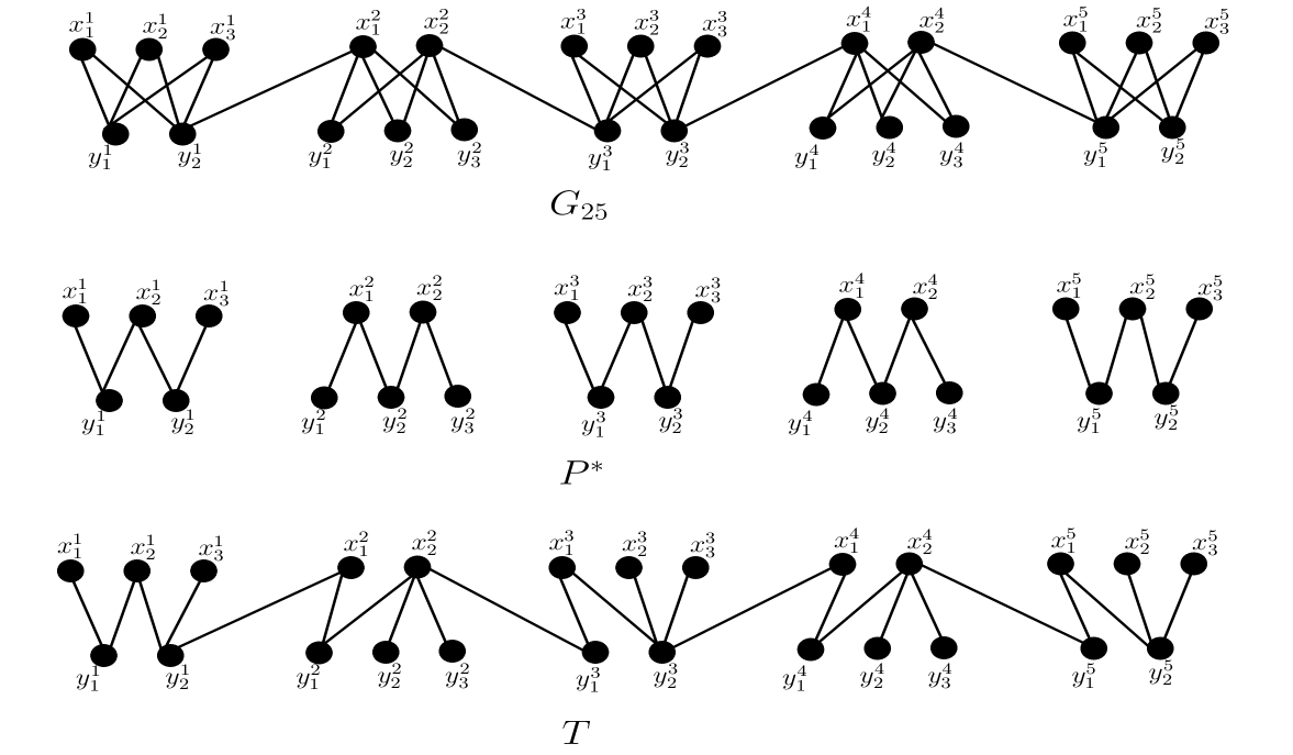
For every integer , we construct a connected bipartite permutation graph with vertices and . For all , let and if is even and and for odd . Let where for all . Let where for each and is the set of edgs of the form if is odd and if is even for each . We see that is a bipartite permutation graph with vertices and edges. Algorithm 3 gives an optimal path cover for having edges and Algorithm 2 gives a MIST with internal vertices. So, we get that . Fig. 11 provides an illustration for .
Thus for bipartite permutation graphs do not have lower bound of the form for some fixed natural number , independent of .
7 Conclusion
We studied the Maximum Internal Spanning Tree (MIST) problem, a generalization of Hamiltonian path problem. As the MIST problem remains NP-hard even for bipartite graphs and chordal graphs due to a reduction from the Hamiltonian path problem [10, 18], we further investigated the complexity of special instances of these classes, chain graphs, bipartite permutation graphs and block graphs. We also investigated cactus graphs and cographs, finding linear-time algorithms for the MIST problem for each of these graph classes.
[15] proved an upper bound for in terms of an optimal path cover. We further studied this relationship between path covers and and showed tight lower bounds for chain graphs and cographs. We also showed this phenomenon does not hold for general graphs with a construction of bipartite permutation graph and block graph such that is arbitrarily far from .
A convex bipartite graph with bipartition and an ordering , is a bipartite graph such that for each , the neighborhood of in appears consecutively. Complexity status of the MIST problem is still open for convex bipartite graphs, which is a superclass of bipartite permutation graphs and subclass of chordal bipartite graphs. Designing an algorithm for MIST in convex bipartite graphs will be a good research direction.
The weighted version of the MIST problem is also well studied in literature [21]. Given a vertex-weighted connected graph , the maximum weight internal spanning tree (MwIST) problem asks for a spanning tree of such that the total weight of internal vertices in is maximized. Since MwIST problem is a generalization of the MIST problem, one may also investigate the complexity status of MwIST problem for some special classes of graphs.
To our knowledge, every known hardness proof for the MIST problem on families of graphs relies on a reduction to Hamiltonian path problem. We leave as an open question if there exists a family of graphs such that Hamiltonian path problem is polynomial time, yet the MIST problem remains NP-hard.
References
- [1] Binkele-Raible D, Fernau H, Gaspers S, Liedloff M, Exact and parameterized algorithms for max internal spanning tree, Algorithmica 65(1) (2013): 95-128.
- [2] Chen ZZ, Harada Y, Guo F, Wang L, An approximation algorithm for maximum internal spanning tree, Journal of Combinatorial Optimization 35(3) (2018): 955-979.
- [3] Cohen N, Fomin FV, Gutin G, Kim E, Saurabh S, Yeo A, Algorithm for finding k-vertex out-trees and its application to k-internal out-branching problem, Journal of Computer and System Sciences 76(7) (2010): 650-662.
- [4] Fomin FV, Gaspers S, Saurabh S, Thomassé S, A linear vertex kernel for maximum internal spanning tree, Journal of Computer and System Sciences 79(1) (2013): 1-6.
- [5] Garey MR, Johnson DS, Computers and intractability, vol 174, freeman San Francisco (1979).
- [6] Heggernes P, Kratsch D, Linear-time certifying recognition algorithms and forbidden induced subgraphs, Nord J Comput 14(1-2) (2007) :87-108.
- [7] Heggernes P, Van’t Hof P, Lokshtanov D, Nederlof J, Computing the cutwidth of bipartite permutation graphs in linear time, SIAM Journal on Discrete Mathematics 26(3) (2012): 1008-1021.
- [8] Jung HA, On a class of posets and the corresponding comparability graphs, Journal of Combinatorial Theory, Series B 24(2) (1978): 125-133.
- [9] Knauer M, Spoerhase J, Better approximation algorithms for the maximum internal spanning tree problem, Algorithmica 71(4)(2015): 797-811.
- [10] Lai TH, Wei SS, The edge hamiltonian path problem is np-complete for bipartite graphs, Information processing letters 46(1) (1993): 21-26.
- [11] Lai TH, Wei SS, Bipartite permutation graphs with application to the minimum buffer size problem, Discrete applied mathematics 74(1) (1997): 33-55.
- [12] Li W, Wang J, Chen J, Cao Y, A 2k-vertex kernel for maximum internal spanning tree, In: Workshop on Algorithms and Data Structures, Springer (2015), pp 495-505.
- [13] Li W, Cao Y, Chen J, Wang J, Deeper local search for parameterized and approximation algorithms for maximum internal spanning tree, Information and Computation 252 (2017):187-200.
- [14] Li X, Zhu D, Approximating the maximum internal spanning tree problem via a maximum path-cycle cover, In: International Symposium on Algorithms and Computation, Springer (2014), pp 467-478.
- [15] Li X, Feng H, Jiang H, Zhu B, Solving the maximum internal spanning tree problem on interval graphs in polynomial time, Theoretical Computer Science 734 (2018): 32-37.
- [16] Lin R, Olariu S, Pruesse G, An optimal path cover algorithm for cographs, Computers and Mathematics with Applications 30(8) (1995): 75-83.
- [17] Lu HI, Ravi R, The power of local optimization: Approximation algorithms for maximum-leaf spanning tree, In: Proceedings of the Annual Allerton Conference on Communication Control and Computing, University of Illinois, (1992), pp 533-533.
- [18] Müller H, Hamiltonian circuits in chordal bipartite graphs, Discrete Mathematics 156(1-3) (1996): 291-298.
- [19] Pak-Ken W, Optimal path cover problem on block graphs, Theoretical computer science 225(1-2) (1999): 163-169.
- [20] Prieto E, Sloper C, Either/or: Using vertex cover structure in designing fpt-algorithms-the case of k-internal spanning tree, In: Workshop on Algorithms and Data Structures, Springer (2003), pp 474-483.
- [21] Salamon G, Approximating the maximum internal spanning tree problem, Theoretical Computer Science 410(50) (2009): 5273-5284.
- [22] Salamon G, Degree-based spanning tree optimization, PhD Thesis (2010).
- [23] Salamon G, Wiener G, On finding spanning trees with few leaves, Information Processing Letters 105(5) (2008): 164-169.
- [24] Seinsche D, On a property of the class of n-colorable graphs, Journal of Combinatorial Theory, Series B 16(2) (1974):191-193.
- [25] Spinrad J, Brandstädt A, Stewart L, Bipartite permutation graphs, Discrete Applied Mathematics 18(3) (1987): 279-292.
- [26] Srikant R, Sundaram R, Singh KS, Rangan CP, Optimal path cover problem on block graphs and bipartite permutation graphs, Theoretical Computer Science 115(2) (1993): 351-357.