Algorithms for Mumford Curves
Abstract.
Mumford showed that Schottky subgroups of give rise to certain curves, now called Mumford curves, over a non-Archimedean field K. Such curves are foundational to subjects dealing with non-Archimedean varieties, including Berkovich theory and tropical geometry. We develop and implement numerical algorithms for Mumford curves over the field of -adic numbers. A crucial and difficult step is finding a good set of generators for a Schottky group, a problem solved in this paper. This result allows us to design and implement algorithms for tasks such as: approximating the period matrices of the Jacobians of Mumford curves; computing the Berkovich skeleta of their analytifications; and approximating points in canonical embeddings. We also discuss specific methods and future work for hyperelliptic Mumford curves.
1. Introduction
Curves over non-Archimedean fields are of fundamental importance to algebraic geometry and number theory. Mumford curves are a family of such curves, and are interesting from both a theoretical and computational perspective. In non-Archimedean geometry, they are quotients of projective space by Schottky groups. In tropical geometry, which looks at the images in of curves under coordinate-wise valuation, these are balanced graphs with the maximal number of cycles. For instance, the tropicalization of an elliptic Mumford curve can be realized as a plane cubic in honeycomb form [CS].
Let be an algebraically closed field complete with respect to a nontrivial non-Archimedean valuation. Unless otherwise stated, will denote a choice of norm on coming from this valuation. Let be the valuation ring of . This is a local ring with unique maximal ideal . Let denote the residue field of . We are most interested in the field of -adic numbers , which unfortunately is not algebraically closed. (For this case, , the ring of -adic integers, and , the field with elements.) Therefore for theoretical purposes we will often consider , the complete algebraic closure of . (In this case is much larger, and is the algebraic closure of .) In most of this paper, choosing elements of that happen to be elements of as inputs for algorithms yields an output once again in . This “ in, out” property means we may take to be for our algorithmic purposes, while still considering when more convenient for the purposes of theory. Much of the theory presented here works for other non-Archimedean fields, such as the field of Puiseux series .
We recall some standard definitions and notation for -adic numbers; for further background on the -adics, see [Ho]. For a prime , the -adic valuation is defined by , where and are not divisible by . The usual -adic norm on is defined for by and for by . This means that large powers of are small in absolute value, and small powers of are large in absolute value. We will usually omit the subscript from both and .
The completion of with respect to the -adic norm is denoted , and is called the field of -adic numbers. Each nonzero element of can be written uniquely as
where , and for all . The -adic valuation and norm extend to this field, and such a sum will have and . In analog to decimal expansions, we will sometimes write
where the expression trails to the left since higher powers of are smaller in -adic absolute value. We may approximate by a finite sum
which will give an error of size at most .
Consider the group , which acts on by treating elements as column vectors. That is, a matrix acts on the point by acting on the vector on the left. Viewed on an affine patch, the elements of this group act as fractional linear transformations. We are interested in the action of certain subgroups of called Schottky groups, because a Schottky group minimally generated by elements will give rise to a curve of genus .
Definition 1.1.
A matrix is hyperbolic if it has two eigenvalues with different valuations. A Schottky group is a finitely generated subgroup such that every non-identity element is hyperbolic.
There are many equivalent definitions of Schottky groups, including the following useful characterization.
Proposition 1.2.
A subgroup of is Schottky if and only if it is free, discrete, and finitely generated. If the generators are elements of , we may replace “free” with “torsion free.”
Let be a Schottky group minimally generated by . The above proposition implies that each element can be written as a unique shortest product , where each . This product is called the reduced word for .
Let be the set of points in that are fixed points of elements of or limit points of the fixed points. The group acts nicely on ; for this reason we will sometimes refer to as the set of bad points for .
Theorem 1.3 (Mumford, [Mu1]).
Let and be as above. Then is analytically isomorphic to a curve of genus . We call such a curve a Mumford curve.
In a companion paper to [Mu1] (see [Mu2]), Mumford also considered abelian varieties over non-Archimedean fields. He showed that these could be represented as , where is called a period matrix for the abelian variety, and represents the multiplicative subgroup generated by its columns.
Since their initial appearance in the 1970s, a rich theory behind Mumford curves has been developed, largely in the 1980s in such works as [GP]. However, prior to the work in this paper there have been few numerical algorithms for working with them (an exception being a treatment of hyperelliptic Mumford curves, mostly genus , in [Ka] from 2007). We have designed and implemented algorithms that accomplish Mumford curve-based tasks over previously absent from the realm of computation, and have made many seemingly theoretical and opaque objects hands-on and tractable.
After discussing in Section 2 a technical hypothesis (“good position”) for the input for our algorithms, we present our main algorithms in Section 3. They accomplish the following tasks, where we denote by :
-
•
Given a Schottky group , find a period matrix for the abelian variety (Algorithm 3.3).
-
•
Given a Schottky group , find a triple , where
-
–
is a graph,
-
–
is a length function on such that the metric graph is the abstract tropical curve which is a skeleton of (the analytification of ), and
-
–
is a natural equivalence from the rose graph on petals;
this data specifies a point in the tropical Teichmüller space described in [CMV] (Algorithm 3.9).
-
–
-
•
Given a Schottky group , find points in a canonical embedding of the curve into (Algorithm 3.13).
In Section 4, we present an algorithm to achieve the “good position” hypothesis that allows the other algorithms to run efficiently, which in doing so verifies that the input group is Schottky (or proves that the group is not Schottky). This is the most important result of this paper, as the algorithms in Section 3 rely heavily upon it.
We take advantage of a property that makes non-Archimedean valued fields like special: . As a result, the error does not accumulate in the computation. Thus we avoid a dangerous hazard present in doing numerical computation over or . The computational problems are hard in nature. Efficient computation for similar problems is not common in the literature even for genus case. Our algorithms are capable of solving genus and some genus examples on a laptop in reasonable time (several minutes). However, they are less efficient for larger cases. The reason is that the running time grows exponentially as the requirement on the precision of the output (in terms of the number of digits) grows. One of the future goals is to find a way to reduce the running time for the algorithms.
Other future goals for Mumford curve algorithms (detailed in Section 5) include natural reversals of the algorithms in Section 3. We are also interested in a particular family of Schottky groups called Whittaker groups, defined in Subsection 5.2. These are the Schottky groups that give rise to hyperelliptic Mumford curves. Some computations for genus curves arising from Whittaker groups were done in [Ka], including computation of Jacobians and finding group representations from ramification points. Two desirable algorithms in this area include:
-
•
Given a Whittaker group , find an affine equation for .
-
•
Given a totally split hyperelliptic curve , find a Whittaker group such that .
The first can be accomplished if a particular presentation of is available, and a brute force algorithm in [Ka] can compute the second if the ramification points of are in a nice position. Future work removing these requirements and improving efficiency would make hyperelliptic Mumford curves very easy to work with computationally.
Acknowledgements
We thank our advisor Bernd Sturmfels for guiding us through this project. We also thank Matthew Baker, Melody Chan, Diane Maclagan and Thomas Scanlon for helpful discussions and communications. Both authors were supported by the National Science Foundation through grant DMS-0968882. Ralph Morrison was also supported in part by UC Berkeley, and in part by the Max Planck Institute for Mathematics in Bonn.
Supplementary Material
We made extensive use of the software package sage [Sage]. Our supplementary files can be found at http://math.berkeley.edu/~ralph42/mumford_curves_supp.html. We have also included the files in the arXiv submission of this paper, and they can be obtained by downloading the source. There are minor changes in the sage implementation from the description of the algorithms in this paper. The changes are made only for convenience in implementation, and they do not affect the behavior of the algorithms.
2. Good fundamental domains in and
This section introduces good fundamental domains and the notion of good position for generators, both of which will play key roles in our algorithms for Mumford curves. Our main algorithms in Section 3 require as input Schottky generators in good position, without which the rate of convergence of approximations will drop drastically. For our method of putting generators into good position, see Section 4.
We start with the usual projective line , then discuss the analytic projective line . Our treatment of good fundamental domains follows Gerritzen and van der Put [GP]. The notion is also discussed by Kadziela [Ka]. The introduction to the analytic projective line follows Baker, Payne and Rabinoff [BPR].
Definition 2.1.
An open ball in is either a usual open ball or the complement of a usual closed ball . A closed ball is either a usual closed ball or the complement of a usual open ball.
The open balls generate a topology on . Both open balls and closed balls are simultaneously open and closed in this topology, as is the case for any non-Archimedean field due to the ultrametric inequality . Let denote the image of under . If , the open ball and the closed ball are distinguished by whether there exist two points in the ball such that equals the diameter. The complement of an open ball is a closed ball, and vice versa.
Definition 2.2.
A good fundamental domain corresponding to the generators is the complement of open balls , such that corresponding closed balls are disjoint, and that and for all . The interior of is . The boundary of is .
The definition above implies that and for all .
Example 2.3.
(1) Let and be the group generated by
Both matrices have eigenvalues and . The matrix has left eigenvectors and , and has left eigenvectors and . We use the convention that . Then, where , , , is a good fundamental domain relative to the generators and . One can verify as follows. First rewrite
Suppose that . Then, , and . So . Also, . So,
So . The other three conditions can be verified similarly.
(2) Let and be the group generated by
Both matrices have eigenvalues and . The matrix has left eigenvectors and , and the matrix has left eigenvectors and . Then, where , , , is a good fundamental domain relative to the generators and .
(3) Let , and let be the group generated by
All three generators have eigenvalues and . The element has eigenvectors and . The element has eigenvectors and . The element has eigenvectors and . Then, where , , , , , is a good fundamental domain relative to the generators , and .
Lemma 2.4.
Let and be as in Definition 2.2, and let and . Write the reduced word for as , where and for all . Assume that if and if . Then we have
Proof.
To simplify notation we’ll outline the proof for the case where for all , and then describe how to generalize to the case of .
Write for each . Since , we know by assumption that . By Definition 2.2 we have , so . By the disjointness of the closed balls, we know that , and since , we have . We may continue in this fashion until we find that .
The only possible obstruction to the above argument in the case of occurs if and (or, similarly, if and , since the above argument needs to act on . However, this situation arises precisely when , meaning that the word is not reduced. Since we’ve assumed is reduced, we have the desired result. ∎
For a fixed set of generators of , there need not exist a good fundamental domain. If there exists a good fundamental domain for some set of free generators of , we say that the generators are in good position. Gerritzen and van der Put [GP, §I.4] proved that there always exists a set of generators in good position. They also proved the following desirable properties for good fundamental domains.
Theorem 2.5.
Let be a Schottky group, its set of bad points, and .
(1) There exists a good fundamental domain for some set of generators of .
Let be a good fundamental domain for , and let .
(2) If , then .
(3) If , then .
(4) .
The statements (2), (3), and (4) imply that can be obtained from by glueing the boundary of . More specifically, is glued with via the action of . We have designed the following subroutine, which takes any point in and finds a point in such that they are equivalent modulo the action of . This subroutine is useful in developing the algorithms in Section 3 and 4.
Subroutine 2.6 (Reducing a point into a good fundamental domain).
Proof.
The correctness of this subroutine is clear. It suffices to prove that the algorithm always terminates. Given , if , by Theorem 2.5, there exists (where each is or for some ) such that . Without loss of generality, we may assume that is chosen such that is the smallest. Steps 3,4 and Lemma 2.4 make sure that we always choose and . Therefore, this subroutine terminates with . ∎
We can extend the definition of good fundamental domains to the analytic projective line . In general, analytification of an algebraic variety is defined in terms of multiplicative seminorms. For our special case , there is a simpler description. As detailed in [Ba], consists of four types of points:
-
•
Type 1 points are just the usual points of .
-
•
Type 2 points correspond to closed balls where .
-
•
Type 3 points correspond to closed balls where .
-
•
Type 4 points correspond to equivalence classes of sequences of nested closed balls such that their intersection is empty.
There is a metric on the set of Type 2 and Type 3 points, defined as follows: let and be two such points and let and be the corresponding closed balls.
-
(1)
If one of them is contained in the other, say is contained in , then the distance is .
-
(2)
In general, there is a unique smallest closed ball containing both of them. Let be the corresponding point. Then, is defined to be .
The metric can be extended to Type 4 points.
This metric makes a tree with infinite branching, as we now describe. There is a unique path connecting any two points and . In case (1) above, the path is defined by the isometry , . It is straightforward to check that . In case (2) above, the path is the concatenation of the paths from to and from to . Then, Type 1 points become limits of Type 2 and Type 3 points with respect to this metric. More precisely, if , then it lies at the limit of the path , . Type 1 points behave like leaves of the tree at infinity. For any two Type 1 points , there is a unique path in connecting them, which has infinite length.
Definition 2.7.
Let be a discrete subset in . The subtree of spanned by , denoted , is the union of all paths connecting all pairs of points in .
An analytic open ball is a subset of whose set of Type 1 points is just and whose Type 2, 3, and 4 points correspond to closed balls and the limit of sequences of such closed balls. An analytic closed ball is similar, with replaced with . Just as in the case of balls in , the analytic closed ball is not the closure of in the metric topology of . The complement of an analytic open ball is an analytic closed ball, and vice versa. In an analytic closed ball such that , the Gaussian point is the Type 2 point corresponding to . An analytic annulus is , where and are analytic balls such that . If is an analytic open (resp. closed) ball and is an analytic closed (resp. open) ball, then is an analytic open annulus (resp. analytic closed annulus). A special case of analytic open annulus is the complement of a point in an analytic open ball.
Any element of sends open balls to open balls and closed balls to closed balls. Thus, there is a well defined action of on .
Definition 2.8.
A good fundamental domain corresponding to the generators is the complement of analytic open balls , such that the corresponding analytic closed balls are disjoint, and that and . The interior of is . The boundary of is .
Definition 2.8 implies that and .
We now argue that there is a one-to-one correspondence between good fundamental domains in and good fundamental domains in . (This fact is well-known, though seldom explicitly stated in the literature; for instance, it’s taken for granted in the later chapters of [GP].) If is a good fundamental domain in , then is a good fundamental domain in . Indeed, since the closed balls are disjoint, and the corresponding analytic closed balls consist of points corresponding to closed balls contained in and their limits, the analytic closed balls are also disjoint. Conversely, if is a good fundamental domain in , then is a good fundamental domain in , because the classical statement can be obtained from the analytic statement by considering only Type 1 points. This correspondence allows us to abuse notation by not distinguishing the classical case and the analytic case. Theorem 2.5 is also true for analytic good fundamental domains.
Another analytic object of interest to us is the minimal skeleton of the analytification of the genus curve (a task that is part of Algorithm 3.9), so we close this section with background information on this object. The following definitions are taken from Baker, Payne and Rabinoff [BPR], with appropriate simplification.
Definition 2.9.
-
(1)
The skeleton of an open annulus is the straight path between the Gaussian point of and the Gaussian point of .
-
(2)
Let be a smooth curve over . A semistable vertex set is a finite set of Type 2 points in such that is the disjoint union of open balls and open annuli. The skeleton corresponding to is the union of with all skeleta of these open annuli.
-
(3)
If , then has a unique minimal skeleton. The minimal skeleton is the intersection of all skeleta. If and is complete, then the minimal skeleton is a finite metric graph. We sometimes call this minimal skeleton the abstract tropical curve of .
Definition 2.10.
An algebraic semistable model of a smooth curve over is a scheme over whose generic fiber is isomorphic to and whose special fiber satisfies
-
•
is a connected and reduced curve, and
-
•
all singularities of are ordinary double points.
Work towards algorithmic computation of semistable models is discussed in such works as [AW, §1.2] and [BW, §3.1], though such computation is in general a hard problem.
Semistable models are related to skeleta in the following way: take a semistable model of . Associate a vertex for each irreducible component of . For each ordinary intersection of two irreducible components in , connect an edge between the two corresponding vertices. The resulting graph is combinatorially a skeleton of .
3. Algorithms Starting With a Schottky Group
If we have a Schottky group in terms of its generators, there are many objects we wish to compute for the corresponding curve , such as the Jacobian of the curve, the minimal skeleton of the analytification of the curve, and a canonical embedding for the curve. In this section we present algorithms for numerically computing these three objects, given the input of a Schottky group with generators in good position. For an algorithm that puts arbitrary generators of a Schottky group into good position, see Section 4.
Remark 3.1.
Several results in this section are concerned with the accuracy of numerical approximations. Most of our results will be of the form
where we think of . This is equivalent to
where . So, since , the size of the error term is a small power of , while the error term itself is a large power of (possibly with a constant that doesn’t matter much).
Rearranging the second equation gives
meaning that we are considering not the absolute precision of our estimate, but rather the relative precision. In this case we would say that our estimate is of relative precision . So if we desire relative precision , we want the actual error term to be (possibly with a constant term with nonnegative valuation), and the size of the error term to be at most .
3.1. The Period Matrix of the Jacobian
Given a Schottky group , we wish to find a period matrix so that . First we’ll set some notation. For any parameters , we introduce the following analytic function in the unknown , called a theta function:
Note that if is defined over and , then . (This is an instance of “ in, out.”) For any and , we can specialize to
It is shown in [GP, II.3] that the function is in fact independent of the choice of . This is because for any choice of we have
From [GP, VI.2] we have a formula for the period matrix of :
Theorem 3.2.
The period matrix for is given by
where is any point in .
As shown in [GP, II.3], the choice of does not affect the value of .
Theorem 3.2 implies that in order to compute each , it suffices to find a way to compute . Since a theta function is defined as a product indexed by the infinite group , approximation will be necessary. Recall that each element in the free group generated by can be written in a unique shortest product called the reduced word, where each . We can approximate by replacing the product over with a product over , the set of elements of whose reduced words have length . More precisely, we approximate with
where
With this approximation method, we are ready to describe an algorithm for computing .
Algorithm 3.3 (Period Matrix Approximation).
The complexity of this algorithm is in the order of the number of elements in , which is exponential in . The next issue is that to achieve certain precision in the final result, we need to know how large needs to be. Given a good fundamental domain for the generators , we are able to give an upper bound on the error in our estimation of by . (Algorithm 3.3 would work even if the given generators were not in good position, but would in general require a very large to give the desired convergence. See Example 3.8(4).)
To analyze the convergence of the infinite product
we need to know where and lie. We can determine this by taking the metric of into consideration. Assume that lies in the interior of . Let be the set of points corresponding to the set of closed balls from the characterization of the good fundamental domain. Let be the smallest pairwise distance between these points. This distance will be key for determining our choice of in the algorithm.
Proposition 3.4.
Let , , and be as above. Suppose the reduced word for is , where . Then for all unless , and unless .
Proof.
We will prove this proposition by induction. If , there is nothing to prove. Let , and assume that the claim holds for all integers with . Without loss of generality, we may assume . Let be the closed disk corresponding to . By Lemma 2.4, we have . This means lies on the unique path from to . Since we assumed , lies on the unique path from to any point in . Thus,
Let if and if . By the same argument as above, lies on the unique path from to . The reducedness of the word guarantees that . So
The last step follows from the inductive hypothesis. The proof of the second part of this proposition is similar. ∎
Proposition 3.5.
Let , , and be as above. Let and such that , , and are distinct modulo the action of . Suppose the reduced word for is . If and , then
Proof.
Our choice of guarantees that both and are in . Without loss of generality, we may assume that . Then, both and are in . So both and lie in , which is contained in some or . By Proposition 3.4, the points in corresponding to the disks and have distance at least . This implies . Therefore, . On the other hand, since and , we have . This means that
as claimed. ∎
We are now ready to prove our approximation theorem, which is a new result that allows one to determine the accuracy of an approximation of a ratio of theta functions. It is similar in spirit to [Ka, Theorem 6.10], which is an approximation result for a particular subclass of Schottky groups called Whittaker groups (see Subsection 5.2 of this paper for more details). Our result is more general, as there are many Schottky groups that are not Whittaker.
Theorem 3.6.
Suppose that the given generators of are in good position, with corresponding good fundamental domain and disks . Let . In Algorithm 3.3, if we choose and such that , then
where is the constant defined above.
Proof.
Our choice of guarantees that both and are in . Thus, if lies in the interior of , then this theorem follows directly from Proposition 3.5. The last obstacle is to remove the assumption on . We observe that is a product of cross ratios:
Therefore, each term is invariant under any projective automorphism of . Under such an automorphism, any point in the interior of can be sent to . ∎
As a special case of this approximation theorem, suppose that we want to compute the period matrix for the tropical Jacobian of , which is the matrix . We need only to compute up to relative precision . Thus, setting suffices. In this case, each of the products , has only one term.
Remark 3.7.
If we wish to use Algorithm 3.3 to compute a period matrix with relative precision (meaning that we want in Theorem 3.6), we must first compute . As above, is defined to be the minimum distance between pairs of the points corresponding to the balls that characterize our good fundamental domain. Once we have computed (perhaps by finding a good fundamental domain using the methods of Section 4), then by Theorem 3.6 we must choose such that , so will suffice.
Example 3.8.
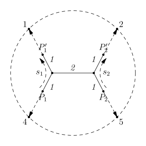
(1) Let be the Schottky group in Example 2.3(1). Choose the same good fundamental domain, with , , , and . The four balls correspond to four points in the tree . We need to find the pairwise distances between the points , , , and in . Since the smallest ball containing both and is , both and are distance from the point corresponding to , so and are distance from one another. Similar calculations give distances of between and , and of between or and or . In fact, the distance between and equals the difference in the valuations of the two eigenvalues of . This allows us to construct the subtree of spanned by as illustrated in Figure 1. The minimum distance between them is . To approximate , we take and . To compute up to relative precision , we need (this is the equation from Remark 3.7), so choosing works. The output of the algorithm is . Similarly, we can get the other entries in the matrix :
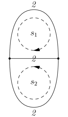
(2) Let be the Schottky group in Example 2.3(2). Choose the same good fundamental domain. Again, we need for relative precision . The algorithm outputs
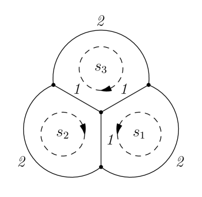
(3) Let be the Schottky group in Example 2.3(3). Choose the same good fundamental domain. The minimum distance between the corresponding points in is , so we may take to have relative precision up to . Our algorithm outputs
(4) Let and be the group generated by
The group is the same as in part (1) of this set of examples, but the generators are not in good position. To achieve the same precision, needs to be up to times greater than in part (1), because the in part (1) now has a reduced word of length . Since the running time grows exponentially in , it is not feasible to approximate using Algorithm 3.3 with these generators as input.
3.2. The Abstract Tropical Curve
This subsection deals with the problem of constructing the corresponding abstract tropical curve of a Schottky group over , together with some data on its homotopy group. This is a relatively easy task, assuming that the given generators are in good position, and that we are also given a fundamental domain . Without loss of generality, we may assume that . Let be the Gaussian points of the disks .
Let be the rose graph on leaves (with one vertex and loops), and let be the loops. A homotopy equivalence must map to loops of that generate , so to specify it will suffice to label such loops of with and orientations. It is for this reason that we call a marking of .
Algorithm 3.9 (Abstract Tropical Curve Construction).
Proof.
The proof is essentially given in [GP, I 4.3]. ∎
Remark 3.10.
It’s worth noting that this algorithm can be done by hand if a good fundamental domain is known. If are the points corresponding to the disjoint closed balls and , then the distance between and is just the sum of their distances from corresponding to , where is the smallest closed ball containing both and . The distance between and is just for . Once all pairwise distances are known, constructing is simple. Finding is simply a matter of drawing the orientation on the loops formed by each pair and labeling that loop . This process is illustrated three times in Example 3.12.
Remark 3.11.
The space parameterizing labelled metric graphs (identifying those with markings that are homotopy equivalent) is called Outer space, and is denoted . It is shown in [CMV] that sits inside tropical Teichmüller space as a dense open set, so Algorithm 3.9 can be viewed as computing a point in tropical Teichmüller space.
Example 3.12.
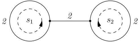
(1) Let be the Schottky group in Example 2.3(1). Choose the same good fundamental domain, with , , , and . We have constructed the subtree of spanned by as illustrated in Figure 1 in Example 3.8(1). After identifying with and with , we get the “dumbbell” graph shown in Figure 1, with both loops having length and the connecting edge having length .


3.3. Canonical Embeddings
From [GP, VI.4], we have that
are linearly independent analytic differentials on that are invariant under the action of . Therefore, they define linearly independent differentials on . Gerritzen and van der Put [GP, VI.4] also state that these form a basis of the space of -invariant analytic differentials. Since the space of algebraic differentials on has dimension , it must be generated by these differentials. Therefore, the canonical embedding has the following form:
It therefore suffices to approximate the derivative . A naïve approach is to consider the approximation
We can do better by taking advantage of the product form of :
Algorithm 3.13 (Canonical Embedding).
With appropriate choice of , we can provide a lower bound on the precision of the result in terms of . Fortunately, we can choose different values of to approximate
for different . As in Proposition 3.5, we choose to ensure that both and are in .
Proposition 3.14.
If we choose in Algorithm 3.13, and assuming , then
where is the minimum pairwise distance between , and is the minimum diameter of .
Proof.
Let have reduced word . We have seen in the proof of Proposition 3.5 that , and , where is one of . Thus,
Since the difference between our approximation and the true value is the sum over terms where has reduced words of length , we conclude that the error has absolute value at most . ∎
In the last proposition, we assumed . If , we can do an extra step and replace by some such that , with the help of Subroutine 2.6. This step does not change the end result because the theta functions are invariant under the action of .
Remark 3.15.
If we wish to use Algorithm 3.13 to compute a period matrix with accuracy up to the -adic digit, we must first compute and . Recall that is defined to be the minimum distance between pairs of the points corresponding to the balls that characterize our good fundamental domain, and is the minimum diameter of . Once we have computed and , then by Proposition 3.14 we must choose such that . We could also think of it as choosing such that .
Remark 3.16.
Example 3.17.
Let be the Schottky group in Example 2.3(3). Choose the same good fundamental domain. We will compute the image of the field element under the canonical embedding (we have chosen as it is in for this particular ). The minimum diameter is , and the minimum distance is . To get absolute precision to the order of , we need , i.e. . Applying Algorithm 3.13 with gives us the following point in :
This point lies on the canonical embedding of the genus Mumford curve . Any genus curve is either a hyperelliptic curve or a smooth plane quartic curve. However, it is impossible for a hyperelliptic curve to have the skeleton in Figure 3 (see [Ch, Theorem 4.15]), so must be a smooth plane quartic curve. Its equation has the form
Using linear algebra over , we can solve for its coefficients by computing points on the curve and plugging them into the equation. The result is
For the Newton subdivision and tropicalization of this plane quartic, see the following subsection, in which we consider the interactions of the three algorithms of Section 3.
3.4. Reality Check: Interactions Between The Algorithms
We close Section 3 by checking that the three algorithms give results consistent with one another and with some mathematical theory. We will use our running example of a genus 3 Mumford curve from Examples 3.8(3), 3.12(3), and 3.17, for which we have computed a period matrix of the Jacobian, the abstract tropical curve, and a canonical embedding.
First we will look at the period matrix and the abstract tropical curve, and verify that these outputs are consistent. Recall that for the period matrix of , we have
Motivated by this, we define
where our choice of does not affect the value of . (Note that .) As shown in [GP, VI, 2], the kernel of is the commutator subgroup of , and is symmetric and positive definite (meaning for any ). Moreover, the following theorem holds (see [Pu2, Theorem 6.4]).
Theorem 3.18.
Let be the abstract tropical curve of , and let be its homotopy group, treating as a topological space. There is a canonical isomorphism such that , where denotes the shared edge length of the oriented paths and .
The map is made very intuitive by considering the construction of in Algoirthm 3.9: a generator of yields two points (corresponding to balls containing the eigenvalues of ), and these points are glued together in constructing . So corresponds to a loop around the cycle resulting from this gluing; after abelianization, this intuition is made rigorous.
Consider the matrix computed in Example 3.8(3). Worrying only about valuations, we have
For , let be the oriented loop in arising from gluing and . In light of Theorem 3.18, we expect to find shared edge lengths
and
That is, each cycle length should be , and the common edge of each distinct pair of cycles should have length , with the orientation of agreeing with the orientation of (respectively, ) on the shared edge and the orientation of disagreeing with the orientation of on the shared edge. This is indeed what we found in Example 3.12(3), with edge lengths and orientations shown in Figure 3. This example has shown how the outputs of Algorithms 3.3 and 3.9 can be checked against one another.
We will now consider the relationship between the abstract tropical curve and the canonical embedding for this example. In particular, we will compute a tropicalization of the curve from the canonical embedding and see how this relates to the abstract tropical curve.
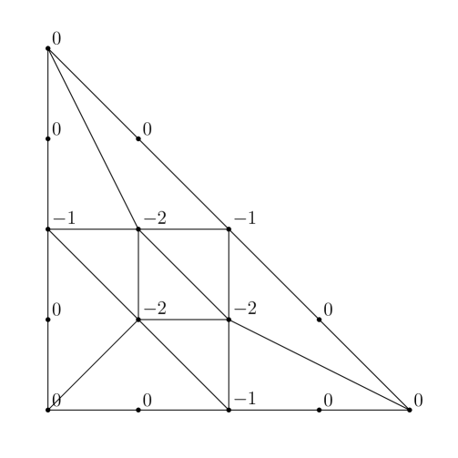
To compute the tropicalization of the curve, we will start with the quartic planar equation computed in Example 3.17. The Newton polytope of this quartic is a triangle with side length . We label each integral point inside or on the boundary of the Newton polytope by the valuation of the coefficient of the corresponding term, ignoring the variable . For example, the point is labeled because the valuation of the coefficient of is . We then take the lower convex hull, giving a subdivision of the Newton polytope as shown in Figure 4. The tropicalization of the curve is combinatorially the dual graph of this polytope, and using the max convention of tropical geometry it sits in as shown in Figure 4, with the common point of the three cycles at .
Let us compare the cycles in the tropicalization with the cycles in the abstract tropical curve. We know from [BPR, §6.23] that this tropicalization is faithful since all vertices are trivalent and are adjacent to at least one edge of weight one. This means that lattice lengths on the tropicalization should agree with lengths of the abstract tropical curve. Each cycle in the tropicalization has five edges, and for each cycle two edges are length and three are length . This gives a length of , as we’d expect based on Example 3.12(3). Moreover, each shared edge has lattice length , as was the case in the abstract tropical curve. Thus we have checked the outputs of Algorithms 3.9 and 3.13 against one another.

4. From Generators in Bad Position to Generators in Good Position
The previous section describes several algorithms that compute various objects from a set of free generators of a Schottky group, assuming that the generators are in good position, and (in Algorithm 3.9) that a good fundamental domain is given together with the generators. This content of this section is what allows us to make this assumption. We give an algorithm (Algorithm 4.8) that takes an arbitrary set of free generators of a Schottky group and outputs a set of free generators that are in good position, together with a good fundamental domain. This algorithm can be modified as described in Remark 4.10 to perform a “Schottky test”; in particular, given a set of invertible matrices generating a group , the modified algorithm will either
-
•
return a set of free generators of in good position together with a good fundamental domain, which is a certificate that is Schottky;
-
•
return a relation satisfied by the input matrices, which is a certificate that the generators do not freely generate the group; or
-
•
return a non-hyperbolic, non-identity matrix , which is a certificate that is not Schottky.
Before presenting Algorithm 4.8, we will first develop some theory for trees, and then define useful subroutines. Our starting point is a remark in Gerritzen and van der Put’s book:
Proposition 4.1.
[GP, III 2.12.3] Let be Schottky and and be as usual. Let be the subtree of spanned by . Then the minimal skeleton of is isomorphic to .
This statement is essential for our algorithm, because it helps reducing problems involving to problems involving the much simpler tree . Though is not finite, it is a finitely branching tree: it consists of vertices and edges such that each vertex is connected with finitely many edges. A good fundamental domain in can be obtained from a good fundamental domain in , defined as follows:
Definition 4.2.
A principal subtree of is a connected component of for some edge of . An extended principal subtree is .
Definition 4.3.
A good fundamental domain in for a set of free generators of is the complement of principal subtrees , such that are disjoint, and that and . The interior of is . The boundary of is .
In other words, is a connected finite subtree of with boundary edges and , where , such that . Given this data, the principal subtree (resp. ) is the connected component of (resp. ) that is disjoint from . Given a good fundamental domain in , one can find a good fundamental domain in as follows. Without loss of generality, we may assume that the retraction of to is in the interior of . Then, and correspond to two nested balls . Define . Define similarly.
Proposition 4.4.
Let be as above. Then is a good fundamental domain.
Proof.
Let be as above. Let be the midpoint of the segment of the boundary edge . Then, corresponds to the ball . Let denote the retraction from to . Again, we may assume is in the interior of . For any , the unique path from to passes through . Therefore, lies on the union of with the segment , which is a subset of . Hence, the condition that and are disjoint implies that the retraction of the and the are disjoint. Thus, the and are disjoint.
Let be the boundary edge of , and let be its midpoint. Since , it sends the midpoint to . Since is a connected component in , the element must send to a connected component of . One of the connected components in is . Since sends to , it must send to . Similarly, sends to . Thus is a good fundamental domain in . ∎
One can establish properties of similar to Theorem 2.5. They can be derived either combinatorially or from Proposition 4.4.
The following algorithm constructs a good fundamental domain in .
Subroutine 4.5 (Good Fundamental Domain Construction).
Proof.
Consider the map from to . Let be as in Step (1). Suppose that a “fire” starts at and the image of in . In each step, when we choose the edge in Step (4) and add a vertex to in Step (5), we “propagate” the fire from to , and “burn” together with halves of all edges connecting to . Also, we “burn” the corresponding part in . Suppose two fires meet each other in . In this case, both halves of an edge in are burned, but it corresponds to two half burned edges in . If so, we stop the fire by removing the edges from and adding them to (Step (9)). The algorithm terminates when the whole graph is burned. The burned part of is a lifting of . Then, is the set of vertices of , is the set of whole edges in , and is the set of half edges in . The fact that they form a good fundamental domain follows from the method in the proof of [GP, I (4.3)]. ∎
This algorithm requires an “agent” knowing everything about . It is hard to construct such an “agent” because is infinite. Therefore, we approximate by a finite subtree. One candidate is , where is the set of fixed points of elements of . Recall that is the set of elements of whose reduced words in terms of the given generators have lengths at most . We take one step further: we approximate by , where is any point in .
Lemma 4.6.
For any , we have . Furthermore, if , then .
Proof.
For any , the fixed point corresponding to the eigenvalue with larger absolute value is the limit of the sequence . The other fixed point is the limit of the sequence . Therefore, every point in is either in or a limit point of . Therefore, . The second statement is clear. ∎
We can construct a complete list of vertices and edges in . Then, the map from to can be approximated in the following way: for each pair of vertices (resp. edges in and each given generator , check if (resp. ). If so, then we identify them. Note that this method may not give the correct map, because two vertices and in may be conjugate via the action of some , where some intermediate step . Due to this flaw, we need a way to certify the correctness of the output.
Subroutine 4.7 (Good Fundamental Domain Certification).
Proof.
Steps 1–4 verify that satisfies the definition of a good fundamental domain in for the set of generators . In addition, we need to verify that generate the same group as the given generators . This is done by Steps 5–9. If in Step 8, then there exists such that . We are assuming in the input, so . Since the action of on is free, we have . Thus, . If for all , then .
Otherwise, if in Step 8 for some , then there exists such that . For any other than identity, we have by a variant of Lemma 2.4. Therefore, . ∎
If the certification fails, we choose a larger and try again, until it succeeds. We are ready to state our main algorithm for this section:
Algorithm 4.8 (Turning Arbitrary Generators into Good Generators).
Proof.
The correctness of the algorithm follows from the proof of Subroutine 4.7. It suffices to prove that the algorithm eventually terminates. Assume that we have the “agent” in Subroutine 4.5. Since Subroutine 4.5 terminates in a finite number of steps, the computation involves only finitely many vertices and edges in . If is sufficiently large, will contain all vertices and edges involved in the computation. Moreover, for any pair of vertices or edges in that are identified in , there exists a sequence of actions by the given generators of that sends one of them to the other, so there are finitely many intermediate steps. If we make even larger so that contains all these intermediate steps, we get the correct approximation of the map . This data is indistinguishable from the “agent” in the computation of Subroutine 4.5. Thus, it will output the correct good fundamental domain. ∎
Remark 4.9.
The performance of the algorithm depends on how “far” the given generator is from a set of generators in good position, measured by the lengths of the reduced words of the good generators in terms of the given generators. If the given generators is close to a set of generators in good position, then a relatively small is sufficient for to contain all relevant vertices. Otherwise, a larger is needed. For example, in the genus case, this algorithm terminates in a few minutes for our test cases where each given generator has a reduced word of length in a set of good generators. However, the algorithm is not efficient on Example 3.8 (4), where one of the given generators has a reduced word of length . One possible way of speeding up the algorithm is to run the non-Euclidean Euclidean algorithm developed by Gilman [Gi] on the given generators.
Remark 4.10.
We may relax the requirement that the input matrices freely generate a Schottky group by checking that every element in not coming from the empty word is hyperbolic before Step 3. If the group is Schottky and freely generated by the input matrices, the algorithm will terminate with a good fundamental domain. Otherwise, Step 7 will never certify a correct good fundamental domain, but the hyperbolic test will eventually fail when a non-hyperbolic matrix is generated. In particular, if the identity matrix is generated by a nonempty word, the generators are not free (though they may or may not generate a Schottky group); and if a non-identity hyperbolic matrix is generated, the group is not Schottky. Thus, Algorithm 4.8 is turned into a Schottky test algorithm. Again, the non-Euclidean Euclidean algorithm in [Gi] is a possible ingredient for a more efficient Schottky test algorithm.
5. Future Directions: Reverse Algorithms and Whittaker Groups
In this section we describe further computational questions about Mumford curves. Algorithms answering these questions would be highly desirable.
5.1. Reversing The Algorithms in Section 3
Many of our main algorithms answer questions of the form “Given , find ”, which we can reverse to “Given B, find .” For instance:
-
•
Given a period matrix , determine if the abelian variety is the Jacobian of a Mumford curve, and if it is approximate the corresponding Schottky group.
-
•
Given an abstract tropical curve , find a Schottky group whose Mumford curve has as its abstract tropical curve.
-
•
Given a polynomial representation of a curve, determine if it is a Mumford curve, and if it is approximate the corresponding Schottky group.
A particular subclass of Schottky groups called Whittaker groups are likely a good starting point for these questions.
5.2. Whittaker Groups
We will outline the construction of Whittaker groups (see [Pu1] for more details), and discuss possible algorithms for handling computations with them. We are particularly interested in going from a matrix representation to a polynomial representation, and vice versa.
If is an element of order , then will have two fixed points, and , and is in fact determined by the pair as
as long as . Let be elements of of order . Write their fixed points as , and assume without loss of generality that for all . Let denote the smallest open balls containing each pair, and assume that the corresponding closed balls are all disjoint. Then the group is in fact the free product .
Note that is not a Schottky group, since its generators are not hyperbolic. However, we can still consider its action upon . To fix some notation, we will choose such that and and will define
(In our previous definition of theta functions, we took to be Schottky, but the definition works fine for this as well.) If we choose and such that , then will be invariant under , which gives a morphism . This will have only one pole, so it is an isomorphism.
Now, let be the kernel of the map defined by for all . Then , and is in fact free on those generators. One can show that is a Schottky group of rank , and we call a group that arises in this way a Whittaker group. We already know that is a curve of genus ; in fact, we have more than that.
Theorem 5.1 (Van der Put, [Pu1]).
If is a Whittaker group, then is a totally split hyperelliptic curve of genus , with affine equation . Conversely, if be a totally split hyperelliptic curve of genus over , then there exists a Whittaker group such that , and this is unique up to conjugation in .
Remark 5.2.
There is a natural map . This is the expected morphism of degree from the hyperelliptic curve to projective space, ramified at points.
If we are content with an algorithm taking as the input representing a Whittaker group (so that ), the above theorem tells us how to compute the ramification points of the hyperelliptic Mumford curve .
Example 5.3.
Let’s construct an example of a Whittaker group of genus with . We need to come up with matrices of order with fixed points sitting inside open balls whose corresponding closed balls are disjoint. We will choose them so that the fixed points of are and ; of are and ; and of are and . (The smallest open balls containing each pair of points has radius , and the corresponding closed balls of radius are disjoint.) The eigenvalues will be and , and the eigenvectors are the fixed points (written projectively), so we can take
So the group
is generated by those three elements of order (and is in fact the free product of the groups , , and ), and its subgroup
is a Whittaker group of rank .
The quotient is a hyperelliptic curve of genus , with six points of ramification , where is the theta function for with suitably chosen and .
Question 1.
As long as we know the -torsion matrices that go into making a Whittaker group, we can find the ramification points of the corresponding hyperelliptic curve. But what if we don’t have that data?
-
•
If we are given , can we algorithmically determine whether or not is Whittaker?
-
•
If we know , can we algorithmically find from ?
-
•
If we know is Whittaker but cannot find , is there another way to find the ramification points of ?
A good first family of examples to consider is Schottky groups generated by two elements. These give rise to genus curves, which are hyperelliptic, so the groups must in fact be Whittaker.
Having discussed going from a Whittaker group to a set of ramification points, we now consider the other direction: going from the ramification points of a totally split hyperelliptic curve and finding the corresponding Whittaker group. This more difficult, though a brute force method was described by Kadziela in [Ka], and was used to compute several genus examples over . We will outline his approach.
After a projective transformation, we may assume that the set of fixed points of the group is of the form
where
and where the generators of are the -torsion matrices with fixed points (taking , , and ). Let us choose parameters for the theta function associated to as and , and write
where
is the sub product of over all matrices in with reduced length exactly .
Theorem 5.4 (Kadziela’s Main Approximation Theorem, [Ka]).
Assume and are as above, and let denote the uniformizer. Then
and for ,
-
•
-
•
-
•
for .
Let be a totally split hyperelliptic curve of genus , which after projective transformation we may assume has its set of ramification points in the form
where . We know for some Whittaker group . To find it will suffice to find the fixed points of the corresponding group , so given we wish to find . We know , but is defined by , and we cannot immediately invert a function we do not yet know. This means we must gradually approximate candidates for both and that give the desired property that . To simplify notation, we will sometimes write instead of in terms of ’s and ’s.
The following algorithm follows the description in [Ka, §6]. Although we have not implemented it, Kadziela used a Magma implementation of it to compute several genus examples over .
Algorithm 5.5 (From Ramification Points to Whittaker Group).
This algorithm is in some sense a brute force algorithm, as for each digit’s place from to it might in principal try every element of , essentially guessing the ’s digit by digit (lines 13 through 24). It is nontrivial that such a brute force method could even work, but this is made possible by Theorem 5.4 as it tells us how to check whether a choice of element in is valid . As with the other algorithms presented in this paper, future algorithms improving the efficiency would be greatly desirable.
References
- [AW] K. Arzdorf and S. Wewers: Another proof of the Semistable Reduction Theorem, arxiv: 1211.4624.
- [Ba] M. Baker: An introduction to Berkovich analytic spaces and non-archimedean potential theory on curves, notes from the 2007 Arizona Winter School on -adic geometry, http://people.math.gatech.edu/~mbaker/pdf/aws07mb_v4.pdf.
- [BPR] M. Baker, S. Payne and J. Rabinoff: Non-archimedean geometry, tropicalization, and metrics on curves, arxiv: 1104.0320.
- [BW] I. Bouw and S. Wewers: Computing -functions and semistable reduction of superelliptic curves, arxiv: 1211.4459.
- [Ch] M. Chan: Tropical Hyperelliptic Curves, J. of Alg. Comb. Volume 37, Issue 2 (2013): 331-359.
- [CMV] M. Chan, M. Melo and F. Viviani: Tropical Teichmüller and Siegel spaces, Proc. of the CIEM workshop in tropical geometry, AMS Contemporary Mathematics 589 (2013), 45-85.
- [CS] M. Chan and B. Sturmfels: Elliptic curves in honeycomb form, Proc. of the CIEM workshop in tropical geometry, AMS Contemporary Mathematics 589 (2013), 87-107.
- [GP] L. Gerritzen and M. van der Put: Schottky groups and Mumford curves, Lect. Notes in Math. 817 (1980).
- [Gi] J. Gilman: The non-Euclidean Euclidean algorithm, arxiv: 1207.1062.
- [Ho] J. Holly: Pictures of ultra metric spaces, the -adic numbers, and valued fields, Amer. Math. Monthly 108.8 (2001), 721-728.
- [Ka] S. Kadziela: Rigid analytic uniformization of hyperelliptic curves, PhD Thesis, University of Illinois at Urbana Champaign (2007).
- [Mu1] D. Mumford: An analytic construction of degenerating curves over complete local rings, Composito Math. 24.2 (1972), 129-174.
- [Mu2] D. Mumford: An analytic construction of degenerating abelian varieties over complete local rings, Composito Math. 24.3 (1972), 239-272.
- [Pu1] M. van der Put: -adic Whittaker groups, Groupe de travail d’analyse ultramétrique 6.15 (1978-1979), 1-6.
- [Pu2] M. van der Put: Discrete groups, Mumford curves and Theta Functions, Annales de la faculté des sciences de Toulouse 6.1 (1992), 399-438.
- [Sage] W. A. Stein et al.: Sage Mathematics Software (Version 5.9), The Sage Development Team, 2013, http://www.sagemath.org.