Alpha-CIR Model with Branching Processes in Sovereign Interest Rate Modelling

Ying Jiao, Chunhua Ma, Simone Scotti Université Claude Bernard-Lyon 1, Institut de Science Financier et d’Assurances. Email: ying.jiao@univ-lyon1.fr.Nankai University, School of Mathematical Sciences. Eamil: mach@nankai.edu.cn.Université Paris Diderot-Paris 7, Laboratoire de Probabilités et Modèles Aléatoires. Email: scotti@math.univ-paris-diderot.fr.

Abstract

We introduce a class of interest rate models, called the $\alpha$ -CIR model, which gives a natural extension of the standard CIR model by adopting the $\alpha$ -stable Lévy process and preserving the branching property. This model allows to describe in a unified and parsimonious way several recent observations on the sovereign bond market such as the persistency of low interest rate together with the presence of large jumps at local extent. We emphasize on a general integral representation of the model by using random fields, with which we establish the link to the CBI processes and the affine models. Finally we analyze the jump behaviors and in particular the large jumps, and we provide numerical illustrations.

1 Introduction

On the current European sovereign bond market, there exists a number of well-established and seemingly puzzling facts. On the one hand, the interest rate has reached a historically low level in the Euro countries. However, on the other hand, the sovereign bond can have very large variations when uncertainty about unpredictable political or economical events increases, such as in the Greek case. The aim of this paper is to present a new model of interest rate, called the $\alpha$ -CIR model, where we give a natural extension of the well-known Cox-Ingersoll-Ross (CIR, see [7]) model by using the $\alpha$ -stable branching processes, in order to describe these recent observations on the bond market. In particular, the set of questions investigated includes the clustering behavior of the variance of sovereign interest rates, and also the persistency of low interest rates together with the significant fluctuations at a local extent.

In the literature, large fluctuations in financial data motivate naturally the introduction of jumps in the interest rate dynamics, such as in Eberlein and Raible [13], Filipović, Tappe and Teichmann [19]. Nevertheless, the jump presence conflicts in general with the trend of low rates, at least as long as the jump intensity is assumed as the paradigm. One way to reconcile large fluctuations with low rate persistency is to use a regime change framework but this may increase the dimension of the stochastic processes in order to preserve the Markov property. Recently, the Hawkes processes or the self-exciting point processes (see Hawkes [23]), have been used to overcome this difficulty since they exhibit properties which give a suitable interpretation of such modelling. A Hawkes process can be seen as a population process whose reproduction rate is proportional to the population itself, that is, the so-called self-exciting property. Moreover, the external arrival of migrant can be modeled by a second point process. A large and growing literature is devoted to the financial application of Hawkes processes, in particular, to the interest rate and credit intensity modelling, such as in Aït-Sahalia, Cacho-Diaz and Laeven [2], Errais, Giesecke and Goldberg [15], Dassios and Zhao [8] and Rambaldi, Pennesi and Lillo [33]. In the above mentioned papers, as appear naturally in Hawkes framework, the driving process is at least two-dimensional since both the dynamics of jump process and its intensity are taken into account.

In this paper, we introduce a short interest rate model by using the $\alpha$ -stable Lévy processes, which provides a relatively simple jump diffusion model to respond to these modelling challenges in an endogenous way. We exploit an integral representation of the $\alpha$ -CIR model to highlight the branching property. First of all, branching processes arise as the limit of Hawkes processes and exhibit, by their inherent nature, the clustering or the self-exciting property implying that the jump frequency increases with the value of the process itself. By consequence, branching processes, thanks to the infinite divisibility of their law with respect to the starting point, prove to be a prolific subject in probability having interesting applications in finance, see for instance Duffie, Filipović and Schachermayer [11]. In the modelling of interest rate, branching processes have already been considered by the pioneering paper of Filipović [17] where the relationship between the exponential affine structure of bond prices and the branching property has been highlighted. Moreover, our model is a natural generalization of the CIR model which appears to be the simplest and most popular continuous-time branching process. Although CIR model has closed-form solutions for bond prices which turns out to be a main feature in view of model calibration, it does not include jumps. In addition, empirical studies underline that the behavior the bond prices cannot be fully explained by CIR model which systematically overestimates short interest rates (see for instance Brown and Dybvig [6] and Gibbons and Ramaswamy [22]). In our framework, CIR process is the departing model which is the only example of branching process with continuous path and the inclusion of the $\alpha$ -stable branching processes allows to better describe the low interest rate behavior.

The main contribution of the present paper is to combine the properties of Hawkes and CIR processes in order to define the $\alpha$ -CIR model, which provides a larger class of jump-diffusion models having the branching property and preserving the explicit expression for bond prices. The $\alpha$ -CIR model consists of, besides the Brownian motion, a spectrally positive $\alpha$ -stable Lévy-process. The parameter $\alpha\in(1,2]$ characterizes the tail fatness and the jump behavior. When $\alpha$ equals $2$ , the $\alpha$ -stable process reduces to a Brownian motion and we recover the classical CIR model. In the general case when $\alpha\in(1,2)$ , there may appear infinitely many jumps in a finite time interval, which represent the fluctuations related to sovereign risks. In order to keep the branching property, the square root in the volatility term have to be replaced by the $\alpha$ -root of the process. Despite its simplicity and the reduced number of extra parameters compared to the usual CIR, the model we develop show several advantages. First, the $\alpha$ -CIR model exhibits positive jumps and, in particular, by combining heavy-tailed jump size distribution with infinite activity, can describe in a unified way both the large fluctuations observed in financial market and the usual small oscillations. Second, in a branching process framework can also be shown that a hierarchical structure for interest rate naturally arises, since it can split the interest rate into different components, which can eventually be interpreted as spreads, each one following the same dynamics, in the similar way in which a global ideal population can be split into subgroups evolving according the same dynamics. Third, by the link established between the $\alpha$ -CIR model and the continuous state branching process with immigration (CBI process), we deduce, using the joint Laplace transform of the CBI process, the bond prices in an explicit way. In particular, we show the interesting result that the bond price increases with the tail fatness (that is, decreases with the parameter $\alpha$ ), which better responds to the persistency of low interest rate behavior of the current sovereign rate. Fourth, we can make a thorough analysis of the jump behavior, in particular, for the large jumps which signify in the interest rate dynamics a sudden increasing sovereign risk and imply, for example in the Greek case, a potentially high probability of default. We are particularly interested in the first time that such a large jump occurs and explore the impact of the tail index $\alpha$ .

We begin our analysis by presenting an equivalence between two different formulations of the dynamics for the $\alpha$ -CIR model. From the theoretical point of view, this property has been thoroughly exploited by Li [30] and Li and Ma [31]. In the spirit of the above papers, we shall prove that the usual version of CIR dynamics and its $\alpha$ -CIR extension admit an alternative representation which is of integral form by using random fields but the dimension of the Lévy basis has to be increased, for instance the Brownian motion is replaced by a two-dimensional white noise. In the financial literature on interest rates, this approach has already been performed, see for example Kennedy [28], Albeverio, Lytvynov and Mahnig [3] where random field modelling is introduced to describe the interest rate term structure. The integral representation allows to better identify the process features like the branching property, and is more convenient for proving related properties. Moreover, it needs to be remarked that the integral representation enlightens the relation between the Ornstein-Uhlenbeck and CIR dynamics, and then between the Lévy-Ornstein-Uhlenbeck (LOU) and $\alpha$ -CIR models. As a matter of fact, in an analogous way that the most natural extension of Ornstein-Uhlenbeck dynamics including branching property is the CIR, the $\alpha$ -CIR results from the combination of the LOU model with $\alpha$ -stable driver and the branching property.

The main, and perhaps most interesting, forecast of the present model is that the bond prices decrease with the parameter $\alpha$ , which in turn is inversely related to the tail fatness. The explanation of this apparently paradoxical result is based on the features of the $\alpha$ -CIR model highlighted previously. The use of fat-tail distributed positive jumps will imply a large negative compensator, then between two jumps the mean reversion term is magnified whenever $\alpha$ decreases. This phenomenon is the consequence of compensation and the final result is to make both tails heavier. In general, the standard behavior of bond prices increases with respect to the fatness of tails, such as the case in ordinary LOU dynamics (see e.g. Barndorff-Nielsen and Shephard [5]). However, for a given value of $\alpha$ , the branching property adds a new phenomenon in the present case with $\alpha$ -CIR model: the frequency of big jumps decreases when interest rates are low thanks to the self-exciting structure and this allows some “freezing” effect of low rates for relatively longer time period. In addition, the strong mean-reverting term resulting in the case of fat-tailed jump distribution will also increase the likelihood of occurrence of the persistency of low rates.

The paper is organized as follows. Section 2 deals with the mathematical presentation of the $\alpha$ -CIR model. Section 3 is devoted to the characterization of our model as a CBI process and the properties derived from this link. In Section 4, we apply our model to term structure modeling and exhibit in particular the closed-form bond prices up to a numerical integration. Section 5 deals with the analysis of jumps. We enrich our results with some numerical illustrations in Section 6. Finally, Section 7 concludes the paper.

2 Model framework

This section introduces the $\alpha$ -CIR interest rate model and its basic properties. We start by defining two representations of our model and establish an explicit link between the two classes, so that the properties of each class are directly transferred to the other one. Let us fix a probability space $(\Omega,\mathcal{F},\mathbb{P})$ equipped with a filtration $\mathbb{F}=(\mathcal{F}_{t})_{t\geq 0}$ satisfying the usual conditions.

Definition 2.1 (Root representation)

We consider the following diffusion for the short interest rate $r=(r_{t},t\geq 0)$ with

r_{t}=r_{0}+\int_{0}^{t}a\left(b-r_{s}\right)ds+\sigma\int_{0}^{t}\sqrt{r_{s}}dB_{s}+\sigma_{Z}\int_{0}^{t}{r_{s-}^{1/\alpha}}dZ_{s}

(1)

where $B=(B_{t},t\geq 0)$ is a Browinan motion and $Z=(Z_{t},t\geq 0)$ is a spectrally positive $\alpha$ -stable compensate Lévy process with parameter $\alpha\in(1,2]$ , which is independent of $B$ and whose Laplace transform is given, for $q\geq 0$ , by

\displaystyle\mathbb{E}\left[e^{-qZ_{t}}\right]=\exp\left\{-\frac{tq^{\alpha}}{\cos(\pi\alpha/2)}\right\}.

In other words, $Z_{t}$ follows the $\alpha$ -stable distribution with scale parameter $t^{1/\alpha}$ , skewness parameter $1$ and zero drift. , i.e., $Z_{t}\sim S_{\alpha}(t^{1/\alpha},1,0)$ .

We call processes defined by (1) the $\alpha$ -CIR processes of parameters $(a,b,\sigma,\sigma_{Z},\alpha)$ and denote by $\alpha$ - $\mathrm{CIR}(a,b,\sigma,\sigma_{Z},\alpha)$ the set of all such processes. The existence of a unique strong solution of the equation (1) follows from Fu and Li [21, Theorem 5.3].

It is easy to see that the CIR model belongs to the class in Definition 2.1 by taking $\sigma_{Z}=0$ . Another case where we recover a CIR process is when $\alpha=2$ . In this case, the process $Z$ becomes a standard Brownian motion scaled by the coefficient $\sqrt{2}$ which is independent of $B$ . Hence an $\alpha$ -CIR process satisfying (1) is actually a CIR process of the form

r_{t}=r_{0}+\int_{0}^{t}a(b-r_{s})\,ds+\sqrt{\sigma^{2}+2\sigma_{Z}^{2}}\int_{0}^{t}\sqrt{r_{s}}d\widetilde{B}_{s}

where $\widetilde{B}=(\sigma B+\sigma_{Z}Z)/\sqrt{\sigma^{2}+2\sigma_{Z}^{2}}$ is a standard Brownian motion. In other words, an $\alpha$ -CIR process with parameter $\alpha=2$ is a CIR process.

The departure of the process ${Z}$ from Brownian motion is controlled by the tail index $\alpha$ . When $\alpha<2$ , ${Z}$ is a pure jump process with heavy tails. For any fixed $t$ , the distribution of $Z_{t}$ is a stable distribution and the tail of the distribution decays like a power function with index $-\alpha$ . This means that a stable random variable exhibits more variability than a Gaussian one and it is more likely to take values far away from the median. Compared to a standard Poisson or compound Poisson process, this pure jump process has an infinite number of (small) jumps over any time interval, allowing it to capture the extreme activity. In the meantime, the $\alpha$ -stable processes share similar properties with the Brownian motion such as self-similarity or stability property, which means that the distribution of the $\alpha$ -stable process over any horizon has the same shape upon scaling. From the statistical point of view, the process given by (1) is characterized by two more parameter with respect to CIR model, i.e. $\alpha$ and $\sigma_{Z}$ .

We then introduce a more general form of the $\alpha$ -CIR model by using random fields.

Definition 2.2 (Integral representation)

We also consider the following equation in the integral form

r_{t}=r_{0}+\int_{0}^{t}a\left(b-r_{s}\right)ds+\sigma\int_{0}^{t}\int_{0}^{r_{s}}W(ds,du)+\sigma_{Z}\int_{0}^{t}\int_{0}^{r_{s-}}\int_{\mathbb{R}^{+}}\zeta\widetilde{N}(ds,du,d\zeta),\quad t\geq 0

(2)

where $W(ds,du)$ is a white noise on $\mathbb{R}_{+}^{2}$ with intensity $dsdu$ , $\widetilde{N}(ds,du,d\zeta)$ is an independent compensated Poisson random measure on $\mathbb{R}_{+}^{3}$ with intensity $dsdu\mu(d\zeta)$ with $\mu(d\zeta)$ being a Lévy measure on $\mathbb{R}_{+}$ and satisfying $\int_{0}^{\infty}(\zeta\wedge\zeta^{2})\mu(d\zeta)<\infty$ .

We call the process given by (2) the $\alpha$ -CIR type process with parameters $(a,b,\sigma,\sigma_{Z},\mu)$ . It follows from of Dawson and Li [10, Theorem 3.1] or Li and Ma [32, Theorem 2.1] that the equation (2) has a unique strong solution.

We establish a first link to the $\alpha$ -CIR model. Let the Lévy measure $\mu$ be as

\displaystyle\mu_{\alpha}(d\zeta)=-{1_{\{\zeta>0\}}d\zeta\over\cos(\pi\alpha/2)\Gamma(-\alpha)\zeta^{1+\alpha}},\quad 1<\alpha<2,

(3)

then the solution of (2) has the same probability law as that of the equation (1). In an extended probability space, for any couple $(B,{Z})$ there exists a couple $(W,\widetilde{N})$ such that the solution of the two equations (2) and (1) are equal almost surely; see Propositions 2.4 and 2.5 below.

Remark 2.3

We explain the connection of the above integral representation to Hawkes processes. We begin by considering an integral representation of the CIR model. Let $W(ds,du)$ be a white noise on $\mathbb{R}_{+}^{2}$ with intensity $dsdu$ . The CIR process $r$ (when $\sigma_{Z}=0$ ) is given in the form $r_{t}=r_{0}+\int_{0}^{t}a\left(b-r_{s}\right)ds+\sigma\int_{0}^{t}\int_{0}^{r_{s}}W(ds,du),$ or equivalently as

\displaystyle r_{t}=r^{\ast}_{t}+\sigma\int_{0}^{t}\int_{0}^{r_{s}}e^{-a(t-s)}W(ds,du)

(4)

where $r^{\ast}_{t}$ is a deterministic function given by $r^{\ast}_{t}=r_{0}e^{-at}+ab\int_{0}^{t}e^{-a(t-s)}ds$ . The expression (4) shows the self-exciting feature.

We then consider a simple Hawkes process with exponential kernel, which is defined as a point process $J$ with intensity $r$ , where $r$ reads

\displaystyle r_{t}=r^{\ast}_{t}+\int_{0}^{t}e^{-a(t-s)}dJ_{s}

and $r^{\ast}$ is the background rate, i.e., the deterministic part of the process $J$ . When a jump arrives, the intensity $r$ increases, which also increases the probability of a next jump, that is the self-exciting property of Hawkes processes. In order to facilitate the comparison with our integral representation, we give a different characterization of the intensity $r$ . Let $N$ be a Poisson process on $\mathbb{R}^{2}$ with characteristic measure $dsdu$ , so $J_{t}$ can be written as the form of $\int_{0}^{t}\int_{0}^{r_{s-}}N(ds,du)$ and $r_{t}$ as

\displaystyle r_{t}=r^{\ast}_{t}+\int_{0}^{t}\int_{0}^{r_{s-}}e^{-a(t-s)}N(ds,du).

(5)

In this form, the self-exciting feature can be observed as follows: the frequency of jumps grows with the process itself due to the presence of the integral with respect to the variable $u$ . Moreover, when $r^{\ast}$ takes certain particular form, $r$ is a branching process, also known as an affine process in finance (see [11]). In this context, the self-exciting features is equivalent to the branching property.

Let us now come back to the integral representation (2) of $\alpha$ -CIR model. We let $\sigma=0$ and $\mu(d\zeta)=\delta_{1}(dz)$ , then the (non-compensated) Poisson measure $N(ds,du,d\zeta)$ reduces to a random measure on $\mathbb{R}_{+}^{2}$ with intensity $dsdu$ , denoted by $N(ds,du)$ . Hence $r$ can be rewritten as

\displaystyle r_{t}=r_{0}+abt-\int_{0}^{t}(a+\sigma_{Z})r_{s}ds+\sigma_{Z}\int_{0}^{t}\int_{0}^{r_{s-}}{N}(ds,du).

We note that $r$ is the intensity of the Hawkes process $\int_{0}^{t}\int_{0}^{r_{s-}}N(ds,du)$ by using the equivalent form

\displaystyle r_{t}=r_{0}e^{-(a+\sigma_{Z})t}+\frac{ab}{a+\sigma_{Z}}\left(1-e^{(a+\sigma_{Z})t}\right)+\int_{0}^{t}\int_{0}^{r_{s-}}e^{-(a+\sigma_{Z})(t-s)}N(ds,du).

(6)

As a consequence, $\alpha$ -CIR type processes, and in particular the $\alpha$ -CIR processes, can be seen as marked Hawkes processes influenced by a Brownian noise.

Furthermore consider a sequence of processes $\big{\{}r_{t}^{(n)},t\geq 0\big{\}}$ defined by (6) with parameters $(a/n,nb,\sigma_{Z})$ . Note that as $n\rightarrow\infty$ , we have

\displaystyle r^{(n)}_{nt}/n\overset{\mathcal{L}}{\longrightarrow}Y_{t},\quad\mbox{in\ }D(\mathbb{R}_{+}),

where $Y$ follows a CIR model given by $Y_{t}=\int_{0}^{t}a(b-Y_{s})ds+\sigma_{Z}\int_{0}^{t}\int_{0}^{Y_{s}}W(ds,du)$ and $D(\mathbb{R}_{+})$ denotes the càdlàg processes space equipped with the Skorokhod topology. Therefore, a sequence of rescaled Hawkes processes converges weakly to the CIR process, see Jaisson and Rosenbaum [29] for more details, notably on the convergence of the nearly unstable Hawkes process with general kernel, after suitably rescaling, to a CIR process.

We now develop the equivalence between the root representation in Definition 2.1 and the integral one in Definition 2.2 with the Lévy measure $\mu_{\alpha}$ . The following two propositions show both implications. The main idea follows [30, Theorem 9.32].

Proposition 2.4

Let $r$ be a solution to (2) with $\mu=\mu_{\alpha}$ given by (3). On an extended probability space of $(\Omega,\mathcal{F},\mathbb{P})$ , there exists a Lévy process $(B,Z)$ valued in $\mathbb{R}^{2}$ where $B$ is a Brownian motion and $Z$ is a spectrally positive $\alpha$ -stable compensated Lévy process, such that $r$ is a solution to (1).

Proof. We extend the probability space to include a standard Brownian motion $\widehat{B}$ and a spectrally positive $\alpha$ -stable compensated Lévy process $\widehat{Z}$ with Lévy measure $\mu_{\alpha}$ as in (3), such that $\widehat{B}$ , $\widehat{Z}$ , $W$ and $\widetilde{N}$ are mutually independent. We then construct the processes $B$ and $Z$ as

B_{t}=\int_{0}^{t}r_{s}^{-1/2}1_{\{r_{s}>0\}}\int_{0}^{r_{s}}W(ds,du)+\int_{0}^{t}1_{\{r_{s}=0\}}d\widehat{B}_{s},\quad t\geq 0

and

Z_{t}=\int_{0}^{t}r_{s-}^{-1/\alpha}1_{\{r_{s-}>0\}}\int_{0}^{\infty}\int_{0}^{r_{s-}}\zeta\widetilde{N}(ds,du,d\zeta)+\int_{0}^{t}1_{\{r_{s-}=0\}}d\widehat{Z}_{s}.

We let $\mathbb{F}=(\mathcal{F}_{t},\,t\geq 0)$ be the filtration generated by these processes. Fix $\theta$ , ${\theta^{\prime}}\in\mathbb{R}$ . Applying Itô’s formula to the two-dimensional martingale $(B,Z)$ we have for $T>t\geq 0$ ,

			$\displaystyle e^{i(\theta B_{T}+\theta^{\prime}Z_{T})}-e^{i(\theta B_{t}+\theta^{\prime}Z_{t})}$
		$\displaystyle=\!\!\!$	$\displaystyle{(M_{T}-M_{t})}-\frac{\theta^{2}}{2}\int_{t}^{T}e^{i(\theta B_{s}+\theta^{\prime}Z_{s})}ds$
			$\displaystyle+\frac{1}{\cos(\pi\alpha/2)\Gamma(-\alpha)}\int_{t}^{T}e^{i(\theta B_{s}+\theta^{\prime}Z_{s-})}1_{\{r_{s-}=0\}}\int_{0}^{\infty}(e^{i\theta^{\prime}\zeta}-1-i\theta^{\prime}\zeta){d\zeta\over\zeta^{1+\alpha}}ds$
			$\displaystyle+\frac{1}{\cos(\pi\alpha/2)\Gamma(-\alpha)}\int_{t}^{T}e^{i(\theta B_{s}+\theta^{\prime}Z_{s-})}r_{s-}1_{\{r_{s-}>0\}}\int_{0}^{\infty}(e^{i\theta^{\prime}r^{-1/\alpha}_{s-}}-1-i\theta^{\prime}r^{-1/\alpha}_{s-}){d\zeta\over\zeta^{1+\alpha}}ds$
		$\displaystyle=\!\!\!$	$\displaystyle(M_{T}-M_{t})+\left[\frac{1}{\cos(\pi\alpha/2)\Gamma(-\alpha)}\int_{0}^{\infty}(e^{i\theta^{\prime}\zeta}-1-i\theta^{\prime}\zeta){d\zeta\over\zeta^{1+\alpha}}-\frac{\theta^{2}}{2}\right]\int_{t}^{T}e^{i(\theta B_{s}+\theta^{\prime}Z_{s})}ds$

where $M$ is a martingale. Then multiplying both sides of the above equality by $e^{-i(\theta B_{t}+\theta^{\prime}Z_{t})}$ and taking conditional expectation, we have that $h_{t}(T):=\mathbb{E}[e^{i(\theta(B_{T}-B_{t})+\theta^{\prime}(Z_{T}-Z_{t}))}|\mathcal{F}_{t}]$ satisfies the integral equation

\displaystyle h_{t}(T)=1+\left[\frac{(\theta^{\prime})^{\alpha}}{\cos(\pi\alpha/2)}e^{-i\pi\alpha/2}-\frac{\theta^{2}}{2}\right]\int_{t}^{T}h_{t}(s)ds,\quad\mbox{a.s.}

Solving the above equation we obtain

\displaystyle\mathbb{E}\left[\left.e^{i(\theta(B_{t}-B_{l})+\theta^{\prime}(Z_{t}-Z_{l}))}\right|\mathcal{F}_{l}\right]=\exp\left\{(t-l)\Big{(}\frac{(\theta^{\prime})^{\alpha}}{\cos(\pi\alpha/2)}e^{-i\pi\alpha/2}-\frac{\theta^{2}}{2}\Big{)}\right\},

which implies that $B$ is a standard Brownian motion and $Z$ is a spectrally positive $\alpha$ -stable compensated Lévy process independent of $B$ . Moreover, by construction $r$ is a solution to (1). $\Box$

Proposition 2.5

Let $r$ be a solution to (1). On an expanded probability space of $(\Omega,\mathcal{F},\mathbb{P})$ , there exist a white noise $W$ on $\mathbb{R}_{+}^{2}$ and a compensated Poisson random measure $\widetilde{N}$ on $\mathbb{R}_{+}^{3}$ with the Lévy measure $\mu_{\alpha}$ given in (3), which are independent, and such that $r$ verifies (2).

Proof. The Lévy-Itô representation of $Z$ implies that $Z_{t}=\int_{0}^{t}\int_{0}^{\infty}\zeta\widetilde{N}(ds,d\zeta)$ , where $\widetilde{N}(ds,dz)$ is a compensated Poisson random measure on $\mathbb{R}_{+}^{2}$ with intensity $ds\mu(d\zeta)$ given by (3). Furthermore, on an extended probability space there exist a white noise $W{{}_{1}}(ds,du)$ on $\mathbb{R}_{+}\times(0,1)$ with intensity $dsdu$ and a Poisson random measure $N_{1}(ds,du,d\zeta)$ on $\mathbb{R}_{+}\times(0,1)\times\mathbb{R}_{+}$ with intensity $dsdu\mu(d\zeta)$ independent of $W_{1}$ such that (c.f. El Karoui and Méléard [14, Corrollary III-5] and Ikeda and Watanabe [25, Theorem 6.7])

\displaystyle B_{t}=\int_{0}^{t}\int_{0}^{1}W_{1}(ds,du)\ \mbox{and}\ \int_{0}^{t}\int_{A}N(ds,d\zeta)=\int_{0}^{t}\int_{0}^{1}\int_{A}N_{1}(ds,du,d\zeta),

(7)

for $A\in\mathcal{B}(\mathbb{R}_{+})$ . In a similar way, on an extended probability space let $W_{2}(du,ds)$ be a white noise on $\mathbb{R}_{+}^{2}$ with intensity $dsdu$ and $N_{2}(ds,du,d\zeta)$ be a Poisson random measure on $\mathbb{R}_{+}^{3}$ with intensity $dsdu{\mu}(d\zeta)$ independent of $W_{2}$ . Then we define for any $A,C\in\mathcal{B}(\mathbb{R}_{+})$ ,

\displaystyle W([0,t]\times A):=\int_{0}^{t}\int_{0}^{1}\sqrt{r_{s}}1_{A}(r_{s}u)W_{1}(ds,du)+\int_{0}^{t}\int_{r_{s}}^{\infty}1_{A}(u)W_{2}(ds,du),

(8)

	$\displaystyle N([0,t]\times A\times C)\!\!\!$	$\displaystyle:=\!\!\!$	$\displaystyle\int_{0}^{t}\int_{0}^{1}\int_{0}^{\infty}1_{A}(r_{s-}u)1_{C}({r_{s-}^{1/\alpha}}\zeta)N_{1}(ds,du,d\zeta)$		(9)
			$\displaystyle+\int_{0}^{t}\int_{r_{s-}}^{\infty}\int_{0}^{\infty}1_{A}(u)1_{C}(\zeta)N_{2}(ds,du,d\zeta).$		(9)

Similarly as in Proposition 2.4, $(W,N)$ has the same distribution as $(W_{2},N_{2})$ . So the proposition is proved. $\Box$

The branching property is one key property of the $\alpha$ -CIR model. The following result shows that the $\alpha$ -CIR process $r$ has the branching property in the pathwise sense, see [10, Theorem 3.2]. The proof is based on the integral representation (2) where the white noise $W$ and the compensated Poisson random measure $\widetilde{N}$ are translation invariant with respect to the variable $u$ .

Proposition 2.6

Let $r$ be an $\alpha$ -CIR $(a,b,\sigma,\sigma_{Z},\alpha)$ process. Let $r_{0}^{(i)}\in\mathbb{R}_{+}$ and $b^{(i)}\in\mathbb{R}$ , $i\in\{1,2\}$ , such that $r_{0}=r_{0}^{(1)}+r_{0}^{(2)}$ and $b=b^{(1)}+b^{(2)}$ . Then there exist independent processes $r^{(i)}$ in the families $\alpha$ -CIR $(a,b^{(i)},\sigma,\sigma_{Z},\alpha)$ with initial values $r_{0}^{(i)}$ such that $r=r^{(1)}+r^{(2)}$ .

Proof. Let $r$ be a solution to (2) with Lévy measure $\mu_{\alpha}$ . Define $r^{(1)}$ to be the solution to the following equation

r_{t}^{(1)}=r_{0}^{(1)}+\int_{0}^{t}a\left(b-r_{s}^{(1)}\right)ds+\sigma\int_{0}^{t}\int_{0}^{r_{s}^{(1)}}W(ds,du)+\sigma_{Z}\int_{0}^{t}\int_{0}^{r_{s-}^{(1)}}\int_{\mathbb{R}^{+}}\zeta\widetilde{N}(ds,du,d\zeta).

(10)

where $(W,N)$ are the same as in (2). Note that $r^{(1)}$ is an $\alpha$ -CIR process with parameters $(a,b^{(1)},\sigma,\sigma_{Z},\alpha)$ . By [10, Theorem 3.2], we have for all $t\geq 0$ , $\mathbb{P}(r_{t}\geq r_{t}^{(1)})=1$ . Let $r^{(2)}=r-r^{(1)}$ . Then

r_{t}^{(2)}=r^{(2)}_{0}+\int_{0}^{t}a\left(b^{(2)}-r^{(2)}_{s}\right)ds+\sigma\int_{0}^{t}\int_{r^{(1)}_{s}}^{r^{(1)}_{s}+r^{(2)}_{s}}W(ds,du)+\sigma_{Z}\int_{0}^{t}\int_{r^{(1)}_{s-}}^{r^{(1)}_{s-}+r^{(2)}_{s-}}\int_{\mathbb{R}^{+}}\zeta\widetilde{N}(ds,du,d\zeta).

By the translation invariance of $W$ and $\widetilde{N}$ with respect to the variable $u$ , we obtain that $r^{(2)}$ is independent of $r^{(1)}$ and is an $\alpha$ -CIR process with parameters $(a,b^{(2)},\sigma,\sigma_{Z},\alpha)$ . The proposition is thus proved. $\Box$

To study the effect of the branching property, we introduce the locally equivalent Lévy-Ornstein-Uhlenbeck (LOU) process to make a comparison with the $\alpha$ -CIR process.

Definition 2.7 (Locally equivalent LOU process)

Let $\lambda=(\lambda_{t},t\geq 0)$ be the solution of the following equation

\lambda_{t}=r_{0}+\int_{0}^{t}a\left(b-\lambda_{s}\right)ds+\sigma\int_{0}^{t}\int_{0}^{r_{0}}W(ds,du)+\sigma_{Z}\int_{0}^{t}\int_{0}^{r_{0}}\int_{\mathbb{R}^{+}}\zeta\widetilde{N}(ds,du,d\zeta),

(11)

where the initial value $r_{0}$ , and the processes $W$ and $\widetilde{N}$ are the same as in Definition 2.2.

Note that, in the case where the Lévy measure is given by $\mu_{\alpha}$ , the process $\lambda$ defined by (11) can be written in the following form as a generalization of the Vasicek model

\lambda_{t}=r_{0}+\int_{0}^{t}a\left(b-\lambda_{s}\right)ds+\sigma\sqrt{r_{0}}B_{t}+\sigma_{Z}\sqrt[\alpha]{r_{0}}Z_{t},

(12)

where $B$ and $Z$ are the same as in Definition 2.1. Comparing (2) and (11), we remark that at the initial time, the two processes have the same volatility and jump terms. But when time evolves, the volatility and jump terms of $\alpha$ -CIR process will be adapted to the actual level of the interest rate, while “frozen” at the initial values in the locally equivalent LOU process.

To further study the difference between (2) and (11), we separate the large and small jumps and use the non-compensated version of the Poisson random measure $\widetilde{N}$ . Since $\alpha$ -stable processes exhibit infinite activity, we fix a jump threshold $y$ (so the threshold for $r$ is given as $\overline{y}=\sigma_{Z}y$ ). The small jumps with infinite activity can be approximated by a second Brownian motion for instance in the spirit of Asmussen and Rosinski [4]. The locally equivalent LOU process reads

	$\displaystyle\lambda_{t}\!\!\!$	$\displaystyle=\!\!\!$	$\displaystyle r_{0}+\int_{0}^{t}a\left(b-\frac{\sigma_{Z}{r_{0}}\Theta(\alpha,y)}{a}-\lambda_{s}\right)ds+\sigma\int_{0}^{t}\int_{0}^{r_{0}}W(ds,du)$		(13)
			$\displaystyle+\sigma_{Z}\int_{0}^{t}\int_{0}^{r_{0}}\int_{0}^{y}\zeta\widetilde{N}(ds,du,d\zeta)+\sigma_{Z}\int_{0}^{t}\int_{0}^{r_{0}}\int_{y}^{\infty}\zeta N(ds,du,d\zeta)\,,$		(13)

where

\Theta(\alpha,y)=-\frac{1}{\cos(\pi\alpha/2)\Gamma(-\alpha)}\int_{y}^{\infty}\frac{d\zeta}{\zeta^{\alpha}}=\frac{2}{\pi}\alpha\Gamma(\alpha-1)\sin(\pi\alpha/2)y^{-(\alpha-1)},

(14)

and $N$ is the (non-compensated) Poisson random measure corresponding to $\widetilde{N}$ . In a similar way, the $\alpha$ -CIR process (2) can be written as

\begin{array}[]{rcl}\displaystyle r_{t}&=&\displaystyle r_{0}+\int_{0}^{t}\widetilde{a}(\alpha,y)\left(\widetilde{b}(\alpha,y)-r_{s}\right)ds+\sigma\int_{0}^{t}\int_{0}^{r_{s}}W(ds,du)\\ &&\quad\displaystyle+\sigma_{Z}\int_{0}^{t}\int_{0}^{r_{s-}}\int_{0}^{y}\zeta\widetilde{N}(ds,du,d\zeta)+\sigma_{Z}\int_{0}^{t}\int_{0}^{r_{s-}}\int_{y}^{\infty}\zeta N(ds,du,d\zeta)\,,\end{array}

(15)

where

\widetilde{a}(\alpha,y)=a+\sigma_{Z}\Theta(\alpha,y)\quad\quad\widetilde{b}(\alpha,y)=\frac{ab}{a+\sigma_{Z}\Theta(\alpha,y)}

(16)

The previous results allow us to make comparisons. First, comparing $\alpha$ -CIR and LOU processes, it follows that the implicit negative drifts from large jump part lead to a linear decay for $\lambda_{t}$ while to a stronger exponential decay for $r_{t}$ . Then as $\sigma_{Z}$ increases, the decreasing drift term plays a more important role in $r_{t}$ than in $\lambda_{t}$ . Second, comparing CIR and $\alpha$ -CIR processes, namely the cases $\sigma_{Z}=0$ and $\sigma_{Z}>0$ in (15), we can study the evolution between two large jumps in the $\alpha$ -CIR model. Between two large jumps, the $\alpha$ -CIR exhibits an increasing mean reverting speed $\widetilde{a}$ and a decreasing long mean interest rate $\widetilde{b}$ as long as $\sigma_{Z}$ increases. As a consequence, the $\alpha$ -CIR diffusion is more adequate to model the presence of low interest rates and their persistency upon large jumps, compared to LOU and CIR models.

We are also interested in the jump times of large jumps. For this purpose, we introduce, based on (15), the auxiliary process

\displaystyle\widehat{r}^{(y)}_{t}=r_{0}+\int_{0}^{t}\widetilde{a}(\alpha,y)\big{(}\widetilde{b}(\alpha,y)-r_{s}\big{)}ds+\sigma\int_{0}^{t}\int_{0}^{r_{s}}W(ds,du)+\sigma_{Z}\int_{0}^{t}\int_{0}^{r_{s-}}\int_{0}^{y}\zeta\widetilde{N}(ds,du,d\zeta).

(17)

For any jump threshold $y>0$ , the process $\widehat{r}^{(y)}$ coincides with $r$ up to the first large jump $\tau_{1}^{(y)}:=\inf\{t>0:\Delta r_{t}>\overline{y}=\sigma_{Z}y\}$ . More generally, denote by $\{\tau_{i}^{(y)}\}_{i\in\mathbb{N}}$ the sequence of jump times of $r$ larger than $\overline{y}$ , then for any $t\in[\tau_{i}^{(y)},\tau_{i+1}^{(y)})$ , we have

\begin{array}[]{rcl}\displaystyle\widehat{r}^{(y)}_{t}&=&\displaystyle r_{\tau_{i}^{(y)}}+\int_{\tau_{i}^{(y)}}^{t}\widetilde{a}(\alpha,y)\big{(}\widetilde{b}(\alpha,y)-\widehat{r}^{(y)}_{s}\big{)}ds+\sigma\int_{\tau_{i}^{(y)}}^{t}\int_{0}^{\widehat{r}^{(y)}_{s}}W(ds,du)\\ &&\displaystyle+\sigma_{Z}\int_{\tau_{i}^{(y)}}^{t}\int_{0}^{\widehat{r}^{(y)}_{s-}}\int_{0}^{y}\zeta\widetilde{N}(ds,du,d\zeta).\end{array}

(18)

This auxiliary process $\widehat{r}^{(y)}$ represents the history of the interest rate $r$ except the jumps larger than $\overline{y}$ . This process will be particularly useful to study $\tau^{(y)}_{1}$ (see Section 5).

3 Link with the CBI processes

In this section, we show that $\alpha$ -CIR processes are continuous state branching processes with immigration (CBI process) and deduce from this fact several properties of the $\alpha$ -CIR model. The CBI processes have been introduced by Kawazu and Watanabe [27]. We recall the definition as below.

Definition 3.1 (CBI process)

A Markov process $X$ with state space $\mathbb{R}_{+}$ is called a continuous state branching process with immigration, characterized by branching mechanism $\Psi(\cdot)$ and immigration rate $\Phi(\cdot)$ , if its characteristic representation is given, for $p\geq 0$ , by

\mathbb{E}_{x}\left[e^{-pX_{t}}\right]=\exp\left[-xv(t,p)-\int_{0}^{t}\Phi\big{(}v(s,p)\big{)}ds\right],

(19)

where the function $v:\mathbb{R}_{+}\times\mathbb{R}_{+}\rightarrow\mathbb{R}$ satisfies the following differential equation

\frac{\partial v(t,p)}{\partial t}=-\Psi(v(t,p)),\quad v(0,p)=p

(20)

and $\Psi$ and $\Phi$ are functions of the variable $q\geq 0$ given by

	$\displaystyle\Psi(q)$	$\displaystyle=$	$\displaystyle\beta q+\frac{1}{2}\sigma^{2}q^{2}+\int_{0}^{\infty}(e^{-qu}-1+qu)\pi(du),$
	$\displaystyle\Phi(q)$	$\displaystyle=$	$\displaystyle\gamma q+\int_{0}^{\infty}(1-e^{-qu})\nu(du),$

with $\sigma,\gamma\geq 0$ , $\beta\in\mathbb{R}$ and $\pi$ , $\nu$ being two Lévy measures such that

\displaystyle\int_{0}^{\infty}(u\wedge u^{2})\pi(du)<\infty,\quad\int_{0}^{\infty}(1\wedge u)\nu(du)<\infty.

(21)

The CBI process $X$ has as generator the operator $\mathcal{L}$ acting on $C^{2}_{0}(\mathbb{R}_{+})$ as

	$\displaystyle\mathcal{L}f(x)$	$\displaystyle=$	$\displaystyle\frac{\sigma^{2}}{2}xf^{\prime\prime}(x)+(\gamma-\beta x)f^{\prime}(x)+x\int_{0}^{\infty}(f(x+u)-f(x)-uf^{\prime}(x))\pi(du)$		(22)
			$\displaystyle\;+\int_{0}^{\infty}\left(f(x+u)-f(x)\right)\nu(du).$		(22)

The next proposition shows that the $\alpha$ -CIR model belongs to the family of CBI processes by using the integral representation (2), see [10, Theorem 3.1]. We shall give two proofs. The first one in the main text is by verification. The second one, which is constructive, is postponed in Appendix.

Proposition 3.2

The $\alpha$ -CIR type process $r$ in Definition 2.2 is a CBI process with the branching mechanism $\Psi$ given by

\Psi(q)=aq+\frac{1}{2}\sigma^{2}q^{2}+\int_{0}^{\infty}(e^{-q\sigma_{Z}\zeta}-1+q\sigma_{Z}\zeta){\mu}(d\zeta)

(23)

and the immigration rate $\Phi(q)=abq$ .

Proof. Let $v(t,p)$ be the unique solution of the differential equation (20) with $\Psi$ given by (23). Fix $t>0$ and let $u(s,p)=v(t-s,p)$ for $0\leq s\leq t$ . Denote by

Y_{s}^{(p)}:=\exp\Big{(}-u(s,p)r_{s}+ab\int_{0}^{s}u(l,p)dl\Big{)}

Applying Itô’s formula, we have that

\displaystyle Y_{t}^{(p)}-Y_{0}^{(p)}-\int_{0}^{t}r_{s}Y_{s}^{(p)}\Big{(}\Psi(u(s,p))-\frac{\partial{u(s,p)}}{\partial{s}}\Big{)}ds,\,t\geq 0

is a martingale. By (20), $(Y_{t}^{(p)}-Y_{0}^{(p)},t\geq 0)$ is a martingale. Thus $\mathbb{E}[Y_{t}^{(p)}]=e^{-u(0,p)r_{0}}$ , which implies that

\displaystyle\mathbb{E}[e^{-pr_{t}}]=\exp\Big{(}{-v(t,p)r_{0}-ab\int_{0}^{t}v(t-s,p)ds}\Big{)}=\exp\Big{(}{-v(t,p)r_{0}-ab\int_{0}^{t}v(s,p)ds}\Big{)}.

Moreover, since $r$ is the unique strong solution of equation (2), it is a Markov process. Thus $r$ is a CBI $(\Psi,\Phi)$ process. $\Box$

As consequence of the previous proposition, the $\alpha$ -CIR model and its truncated process are both CBI processes by considering particular Lévy measures.

Corollary 3.3

The $\alpha$ -CIR $(a,b,\sigma,\sigma_{Z},\alpha)$ process is a CBI process with the branching mechanism $\Psi$ given by

\Psi_{\alpha}(q)=aq+\frac{\sigma^{2}}{2}q^{2}-\frac{\sigma_{Z}^{\alpha}}{\cos(\pi\alpha/2)}q^{\alpha},

(24)

and the immigration rate $\Phi$ given by

\Phi(q)=abq.

(25)

Corollary 3.4

The auxiliary process $\widehat{r}^{(y)}$ defined by (17) is a CBI process with the branching mechanism $\Psi^{(y)}$ given by

\Psi^{(y)}_{\alpha}(q):=\Big{(}a+\sigma_{Z}^{\alpha}\int_{y}^{\infty}\zeta\mu_{\alpha}(d\zeta)\Big{)}q+\frac{1}{2}\sigma^{2}q^{2}+\sigma_{Z}^{\alpha}\int_{0}^{y}(e^{-q\zeta}-1+q\zeta)\mu_{\alpha}(d\zeta),

(26)

where $\mu_{\alpha}$ is given by (3) and the immigration rate $\Phi$ given by

\Phi(q)=\widetilde{a}(\alpha,y)\,\widetilde{b}(\alpha,y)\,q=ab\,q.

(27)

In the following of this section, we use the CBI characterization to show some properties of the $\alpha$ -CIR model.

Proposition 3.5

Let $(r^{(\alpha)}_{t},t\geq 0)$ denote the $\alpha$ -CIR process with parameters $(a,b,\sigma,\sigma_{Z},\alpha)$ . Then as $\alpha\rightarrow 2$ , $r^{(\alpha)}$ converges in distribution in $D(\mathbb{R}_{+})$ to the CIR process $r^{(2)}$ .

Proof. For any $\alpha\in(1,2]$ , the $\alpha$ -CIR process $r^{(\alpha)}$ is a CBI process. Let $P^{(\alpha)}$ be the transition semigroup of $r^{(\alpha)}$ and $A^{(\alpha)}$ be its generator. Denote $e_{p}(x)=e^{-px}$ for $p>0$ and $x\geq 0$ . Then by (22),

A^{(\alpha)}e_{p}(x)=-e_{p}(x)\left(x\Psi_{\alpha}(p)+\Phi(p)\right)=-e^{-px}\Big{(}x\big{(}ap+\frac{\sigma^{2}}{2}p^{2}-\frac{\sigma_{Z}^{\alpha}}{\cos(\pi\alpha/2)}p^{\alpha}\big{)}+abp\Big{)}.

We have

\displaystyle\lim_{\alpha\rightarrow 2}\,\sup_{x\in\mathbb{R}_{+}}|A^{(\alpha)}e_{p}(x)-A^{(2)}e_{p}(x)|=0.

Denote by $D_{1}$ the linear hull of $\{e_{p}:p>0\}$ . Then $D_{1}$ is an algebra which strongly separates the points of $\mathbb{R}_{+}$ . Let $C_{0}(\mathbb{R}_{+})$ be the space of continuous functions on $\mathbb{R}_{+}$ vanishing at infinity. By the Stone-Weierstrass theorem, $D_{1}$ is dense in $C_{0}(\mathbb{R}_{+})$ . Since $D_{1}$ is invariant under $P^{(2)}$ (see (19)), it is a core of $A^{(2)}$ (see Ethier and Kurtz [16, Proposition 3.3]). By [16, Corollary 8.7], we have the weak convergence of the processes as $\alpha$ tends to $2$ . $\Box$

Proposition 3.6

The $\alpha$ -CIR type process in Definition 2.2 has a limit distribution, whose Laplace transform is given by

\displaystyle\mathbb{E}[e^{-pr_{\infty}}]=\exp\Big{(}-\int_{0}^{p}\frac{\Phi(q)}{\Psi(q)}dq\Big{)},\quad p\geq 0.

(28)

Moreover, the process is exponentially ergodic, namely $\|\mathbb{P}(r_{t}\in\,\cdot\,)-\mathbb{P}(r_{\infty}\in\,\cdot\,)\|\leqslant C\rho^{t}$ for some positive constants $C$ and $\rho<1$ , where $\|\cdot\|$ denotes the total variation norm.

Proof. Note that the branching mechanism $\Psi$ is bounded from below by $aq+\frac{1}{2}\sigma^{2}q^{2}$ . Hence one has

\int_{0}^{1}\frac{\Phi(q)}{\Psi(q)}dq\leqslant\int_{0}^{1}\frac{abq}{aq+\frac{1}{2}\sigma^{2}q^{2}}dq<\infty.

By [30, Theorem 3.20], we obtain that the process $r$ in Definition 2.2 has a limit distribution, whose Laplace transform is given by $\exp\big{(}-\int_{0}^{\infty}\Phi(v(t,p))dt\big{)}$ , where the function $v$ is defined in (20). A change of variables $q=v(t,p)$ in the above formula leads to (28). The last assertion follows from [32, Theorem 2.5]. $\Box$

Finally, we show that the usual condition of inaccessibility of the point $0$ is preserved when we extend CIR model to the $\alpha$ -CIR one.

Proposition 3.7

For the $\alpha$ -CIR $(a,b,\sigma,\sigma_{Z},\alpha)$ process with $\alpha\in(1,2)$ , the point $0$ is an inaccessible boundary if and only if $2ab\geq\sigma^{2}$ . In particular, a pure jump $\alpha$ -CIR process with $ab>0$ never reaches $0$ .

Proof. We apply the result of Duhalde, Foucart and Ma [12, Theorem 2] for CBI processes to obtain that $0$ is an inaccessible boundary point for an $\alpha$ -CIR type process if and only if

\displaystyle\int_{\theta}^{\infty}\frac{dz}{\Psi(z)}\exp\Big{(}\int_{\theta}^{z}\frac{\Phi(x)}{\Psi(x)}dx\Big{)}=\infty

(29)

for some positive constant $\theta$ , where $\Psi$ is given by (23) and $\Phi(q)=abq$ . We now focus on the $\alpha$ -CIR process. Let $\Psi^{*}(q)=aq+\sigma^{2}q^{2}/2$ be the branching mechanism of the classical CIR process viewed as a CBI process. One has $\Psi_{\alpha}\geq\Psi^{*}$ , where $\Psi_{\alpha}$ is the branching mechanism of the $\alpha$ -CIR process, given in (24). Therefore

\int_{\theta}^{\infty}\frac{dz}{\Psi_{\alpha}(z)}\exp\Big{(}\int_{\theta}^{z}\frac{\Phi(x)}{\Psi_{\alpha}(x)}dx\Big{)}\leq\int_{\theta}^{\infty}\frac{dz}{\Psi^{*}(z)}\exp\Big{(}\int_{\theta}^{z}\frac{\Phi(x)}{\Psi^{*}(x)}dx\Big{)}.

In particular, if $0$ is an inaccessible boundary for the $\alpha$ -CIR $(a,b,\sigma,\sigma_{Z},\alpha)$ process, then the inequality $2ab\geq\sigma^{2}$ holds, thanks to the classical inaccessibility criterion for the CIR processes.

Conversely, if the inequality $2ab\geq\sigma^{2}$ holds, then one has

\frac{\Phi(x)}{\Psi_{\alpha}(x)}=\frac{1}{x}(1+O(x^{\alpha-2})),\quad x\rightarrow+\infty.

So there exists a constant $C>0$ (depending on $\theta$ ) such that

\int_{\theta}^{z}\frac{\Phi(x)}{\Psi_{\alpha}(x)}dx\geq\log(z/\theta)-C.

Hence

\int_{\theta}^{\infty}\frac{dz}{\Psi_{\alpha}(z)}\exp\Big{(}\int_{\theta}^{z}\frac{\Phi(x)}{\Psi_{\alpha}(x)}dx\Big{)}\geqslant\frac{1}{e^{C}\theta}\int_{\theta}^{\infty}\frac{z}{\Psi_{\alpha}(z)}dz=+\infty.

$\Box$

Remark 3.8

The result of Proposition 3.7 is not true when $\alpha=2$ . In this case the $\alpha$ -CIR model reduces to a classical CIR model, but with a modified volatility term. Therefore for the $\alpha$ -CIR $(a,b,\sigma,\sigma_{Z},2)$ process, the point $0$ is an inaccessible boundary if and only if $2ab\geq\sigma^{2}+2\sigma_{Z}^{2}$ . We note that when the $\alpha$ -CIR process contains the jump part, the parameter $\sigma_{Z}$ does not intervene in the boundary condition by the above proposition.

4 Applications to interest rate modeling

In this section, we apply the $\alpha$ -CIR model to the interest rate modelling and pricing. Since the $\alpha$ -CIR model is a generalization of the classical CIR model by adding jumps but preserving the CBI properties, the bond price has an affine structure, see Filipović [17]. We give a closed-form expression of the bond price depending on a function which is the integral of the reciprocal of $1-\Psi_{\alpha}$ . This integral can be easily computed numerically, and so is semi-explicit formula for the Laplace transform of the integrated interest rate. Moreover, we show that the bond price is decreasing with respect to the index parameter $\alpha$ . In the next part, we focus on a path dependent option, more precisely a put option written on the running minimum of the bond yield. We show that the payoff of this option can be rewritten as a put option written on the running minimum of the spot rate itself with different nominal and strike. Despite the non-Markovian behavior and the non linearity of the payoff, its price can be obtained by inversion of the Laplace transform.

4.1 Zero-coupon bond pricing

We begin by making precise the equivalent probability measures. The following proposition shows that the short interest rate $r$ , given by the $\alpha$ -CIR model, remains to be in the class of integral type processes under an equivalent change of probability.

Proposition 4.1

Let $r$ be an $\alpha$ -CIR $(a,b,\sigma,\sigma_{Z},\alpha)$ processes under the probability measure $\mathbb{P}$ and assume that the filtration $\mathbb{F}$ is generated by the random fields $W$ and $\widetilde{N}$ . Fix $\eta\in\mathbb{R}$ and $\theta\in\mathbb{R}_{+}$ , and define

\displaystyle U_{t}:=\eta\int_{0}^{t}\int_{0}^{r_{s}}W(ds,du)+\int_{0}^{t}\int_{0}^{r_{s-}}\int_{0}^{\infty}(e^{-\theta\zeta}-1)\widetilde{N}(ds,du,d\zeta).

Then the Doléans-Dade exponential $\mathcal{E}(U)$ is a martingale and the probability measure $\mathbb{Q}$ defined by

\displaystyle\left.\frac{d\mathbb{Q}}{d\mathbb{P}}\right|_{\mathcal{F}_{t}}=\mathcal{E}(U)_{t},

is equivalent to $\mathbb{P}$ . Moreover, under $\mathbb{Q}$ , $r$ is an $\alpha$ -CIR type process with the parameters $(a^{\prime},b^{\prime},\sigma^{\prime},\sigma_{Z}^{\prime},\mu_{\alpha}^{\prime})$ , where

a^{\prime}=a-\sigma\eta-\frac{\alpha\sigma_{Z}}{\cos(\pi\alpha/2)}\theta^{\alpha-1},\quad b^{\prime}=ab/a^{\prime},\quad\sigma^{\prime}=\sigma,\quad\sigma_{Z}^{\prime}=\sigma_{Z}

and

\displaystyle\mu_{\alpha}^{\prime}(d\zeta)=-\frac{e^{-\theta\zeta}}{\cos(\pi\alpha/2)\Gamma(-\alpha)\zeta^{1+\alpha}}d\zeta.

Proof. The couple $(r,U)$ is a time homogeneous affine process (c.f. [9, Theorem 6.2]). The Doléans-Dade exponential $\mathcal{E}(U)$ is a true martingale by checking that the conditions in [26, Corollary 3.2] are satisfied, so it defines an equivalent probability measure $\mathbb{Q}$ . Note that $Y=\mathcal{E}(U)$ is the unique strong solution of $dY_{t}=Y_{t-}dU_{t}$ . Then for any function $f\in C^{2}(\mathbb{R_{+}})$ , the process

	$\displaystyle Y_{t}f(r_{t})-\int_{0}^{t}Y_{s}f^{\prime}(r_{s})\bigg{(}ab-\Big{(}a-\sigma\eta-\sigma_{Z}\int_{0}^{\infty}\zeta(e^{-\theta\zeta}-1)\mu_{\alpha}(d\zeta)\Big{)}r_{s}\bigg{)}ds-\frac{\sigma^{2}}{2}\int_{0}^{t}Y_{s}f^{\prime\prime}(r_{s})r_{s}ds$
	$\displaystyle\quad\quad\quad-\int_{0}^{t}Y_{s}r_{s}ds\int_{0}^{\infty}\Big{(}f(r_{s-}+\sigma_{Z}\zeta)-f(r_{s})-f^{\prime}(r_{s-})\sigma_{Z}\zeta\Big{)}e^{-\theta\zeta}\mu_{\alpha}(d\zeta),\quad t\geq 0$

is a local martingale, which implies that under $\mathbb{Q}$ , $r$ is an $\alpha$ -CIR type process with the parameters $(a^{\prime},b^{\prime},\sigma^{\prime},\sigma_{Z}^{\prime},\mu_{\alpha}^{\prime})$ . $\Box$

Remark 4.2

Usually we choose $\eta$ and $\theta$ such that $a^{\prime}>0$ . When $\theta=0$ , $\mu_{\alpha}^{\prime}$ coincides with $\mu_{\alpha}$ given in (3), so that an $\alpha$ -CIR process will remain in the same class under an equivalent change of probability measure. When $\theta>0$ , the $\alpha$ -CIR process becomes an $\alpha$ -CIR type process driven by a tempered stable process under the change of probability measure. In this case, we can apply the following result on the general CBI processes to compute the bond prices.

As highlighted by Filipović [17, 18], a large class of bond options admits a nice expression via the exponential affine transformation, see [18, Theorem 10.5] and [17, Section 6]. The next proposition gives a general result about the joint Laplace transform of a CBI process and its integrated process, which will be useful for the bond pricing.

Proposition 4.3

Let $X$ be a CBI $(\Psi,\Phi)$ process given by (19) with $X_{0}=x$ . For non-negative real numbers $\xi$ and $\theta$ , we have

\displaystyle{\mathbb{E}}_{x}\Big{[}e^{-\xi X_{t}-\theta\int_{0}^{t}X_{s}ds}\Big{]}=\exp\Big{(}-xv(t,\xi,\theta)-\int_{0}^{t}\Phi\big{(}v(s,\xi,\theta)\big{)}ds\Big{)},

(30)

where $v(t,\xi,\theta)$ is the unique solution of

\displaystyle\frac{\partial v(t,\xi,\theta)}{\partial t}=-\Psi(v(t,\xi,\theta))+\theta,\quad v(0,\xi,\theta)=\xi.

(31)

Proof. For any function $f\in C^{2}(\mathbb{R_{+}})$ , $(f(X_{t})-f(x)-\int_{0}^{t}\mathcal{L}f(X_{s})ds,\;t\geq 0)$ is a local martingale, where the operator $\mathcal{L}$ given by (22). Then

\displaystyle f(X_{t})e^{-\theta\int_{0}^{t}X_{s}ds}-f(x)-\int_{0}^{t}{e^{-\theta\int_{0}^{t}X_{s}ds}}\big{(}\mathcal{L}f(X_{s})-\theta X_{s}f(X_{s})\big{)}ds,\quad t\geq 0

is also a local martingale. Denote the Feynman-Kac semigroup by $Q_{t}$ and the corresponding process by $\overline{X}$ as follows:

\displaystyle Q_{t}f(x)=\overline{\mathbb{E}}_{x}\left[f\left(\overline{X}_{t}\right)\right]:=\mathbb{E}_{x}\Big{[}f(X_{t})e^{-\theta\int_{0}^{t}X_{s}ds}\Big{]}.

Then $\overline{X}$ is a non-conservative (in other words the process may explode in finite time) CBI process with generator defined by $\mathcal{A}f(x)=\mathcal{L}f(x)-\theta xf(x)$ by [27, Theorem 1.1] and implies in addition that

\displaystyle\overline{\mathbb{E}}_{x}[e^{-\xi\overline{X}_{t}}]=\exp\Big{(}-xv(t,\xi,\theta)-\int_{0}^{t}\Phi(v(s,\xi,\theta))ds\Big{)},

where $v(\cdot,\xi,\theta)$ is the unique solutions of

\displaystyle\frac{\partial v(t,\xi,\theta)}{\partial t}=-\Psi(v(t,\xi,\theta))+\theta,\quad v(0,\xi,\theta)=\xi.

The proposition is thus proved. $\Box$

The above proposition allows to compute the zero-coupon bond price with a short rate driven by $\alpha$ -CIR model, under an equivalent probability measure. In the following, we give the zero-coupon price when the short rate $r$ satisfies the $\alpha$ -CIR model of parameter $(a,b,\sigma,\sigma_{Z},\alpha)$ under the equivalent risk-neutral probability $\mathbb{Q}$ , and analyze its decreasing property with respect to $\alpha$ . Recall that the value of a zero-coupon bond of maturity $T$ at time $t\leq T$ is given by

B(t,T)=\mathbb{E}^{\mathbb{Q}}\Big{[}\exp\Big{(}-\int_{t}^{T}r_{s}ds\Big{)}\,|\,\mathcal{F}_{t}\Big{]}.

(32)

For the sake of simplicity, we will use the notation $\mathbb{E}$ in place of $\mathbb{E}^{\mathbb{Q}}$ .

Proposition 4.4

Let the short rate $r$ be given by the $\alpha$ -CIR model (1) under the probability measure $\mathbb{Q}$ . Then the zero-coupon bond price is given by

B(t,T)=\exp\Big{(}-r_{t}v(T-t)-ab\int_{0}^{T-t}v(s)ds\Big{)},

(33)

where $v(s)$ is the unique solution of the equation

\displaystyle\frac{\partial v(t)}{\partial t}=1-\Psi_{\alpha}(v(t)),\quad v(0)=0,

(34)

with $\Psi_{\alpha}(q)=aq+\frac{\sigma^{2}}{2}q^{2}-\frac{\sigma_{Z}^{\alpha}}{\cos(\pi\alpha/2)}q^{\alpha}$ as in (24). Moreover, we have

v(t)=f^{-1}(t)\,\text{ where }\,f(t)=\int_{0}^{t}\frac{dx}{1-\Psi_{\alpha}(x)}

(35)

Proof. Applying Propositions 4.3 with $\xi=0$ and $\theta=1$ , we have

\mathbb{E}\left[\left.e^{-\int_{t}^{T}r_{s}ds}\right|\mathcal{F}_{t}\right]=\exp\Big{(}-r_{t}v(T-t)-ab\int_{0}^{T-t}v(s)ds\Big{)},

where $v(t)$ is the unique solution of (34) with $\Psi_{\alpha}$ given in (24). Since $\Psi_{\alpha}(\cdot)$ is a nonnegative, increasing and convex function, the equation $\Psi_{\alpha}(x)=1$ has the unique solution denoted by $x_{0}$ . For $0\leq x<x_{0}$ , $1-\Psi_{\alpha}(x)>0$ . Note that $f(u)$ is strictly increasing in $u\in[0,x_{0})$ and $f(u)\rightarrow\infty$ as $u\rightarrow x_{0}$ . It follows from (34) that

\displaystyle\int_{0}^{v(t)}\frac{dv}{1-\Psi_{\alpha}(v)}=t.

Let $t$ tend to infinity on both sides of the above equality. Then $v(t)\rightarrow x_{0}$ as $t\rightarrow\infty$ and $v(t)<x_{0}$ for any $t\geq 0$ . Also by (34), $v(t)$ is strictly increasing. So one has $v(t)=f^{-1}(t)$ . $\Box$

Proposition 4.5

The function $v$ is increasing with respect to $\alpha\in(1,2]$ . In particular, the bond price $B(0,T)$ is decreasing with respect to $\alpha$ .

Proof. We write the function $v$ as $v(t,\alpha)$ to emphasize the dependence on the parameter $\alpha$ . Since $1-\Psi_{\alpha}(u)$ is a decreasing concave function of $u$ and $\Psi_{\alpha}(0)=0$ , there is a unique positive solution, denoted by $v^{*}(\alpha)$ , to the equation $1-\Psi_{\alpha}(u)=0$ . It is not hard to see that $0\leq v(s,\alpha)<v^{*}(\alpha)$ and $\lim_{t\rightarrow\infty}v(s,\alpha)=v^{*}(\alpha)$ . Moreover, from the relation $1-\Psi_{\alpha}(v^{*}(\alpha))=0$ we obtain that $(\sigma_{Z}v^{*}(\alpha))^{\alpha}\leq-\cos(\pi\alpha/2)\leq 1$ and hence $\sigma_{Z}v^{*}(\alpha)\leq 1$ .

For any $t\in\mathbb{R}_{+}$ , one has

t=\int_{0}^{v(t,\alpha)}\frac{dx}{1-\Psi_{\alpha}(x)}.

Taking the derivative with respect to $\alpha$ , we obtain

\frac{1}{1-\Psi_{\alpha}(v(t,\alpha))}\cdot\frac{\partial v}{\partial\alpha}(t,\alpha)+\int_{0}^{v(t,\alpha)}\frac{1}{(1-\Psi_{\alpha}(x))^{2}}\cdot\frac{\partial\Psi_{\alpha}}{\partial\alpha}(x)dx=0.

Note that by (24),

\frac{\partial\Psi_{\alpha}}{\partial\alpha}(x)=-\frac{\sin(\pi\alpha/2)}{\cos^{2}(\pi\alpha/2)}\Big{(}\frac{\pi}{2}\Big{)}(\sigma_{Z}x)^{\alpha}-\frac{(\sigma_{Z}x)^{\alpha}}{\cos(\pi\alpha/2)}\ln(\sigma_{Z}x)\leq 0

on $x\in(0,v^{*}(\alpha)]$ since $\sigma_{Z}v^{*}(\alpha)\leq 1$ and $\cos(\pi\alpha/2)<0$ . Therefore we obtain $\partial v/\partial\alpha\geq 0$ , namely the function $v$ is increasing with respect to $\alpha$ . In particular, the bond price $B(0,T)$ is a decreasing function of $\alpha$ . $\Box$

Proposition 4.5 shows that the $\alpha$ -CIR model with $\alpha<2$ permits to capture the low interest rate behavior from the point of view of bond pricing. This result is surprising at first sight since the parameter $\alpha$ is an inverse measure of heaviness of distribution tails, more as $\alpha$ close to $1$ , more likely that the large jumps appear (see also Section 5). In addition, in the $\alpha$ -CIR model, $\alpha$ coincides with the so-called generalized Blumenthal-Getoor index which is defined as $\inf\{\beta>0:\sum_{0\leq s\leq T}\Delta r_{s}^{\beta}<\infty,\ a.s.\}$ with $\Delta r_{s}:=r_{s}-r_{s-}$ and $T$ a horizon time (see e.g. [1]) and is often used to measure the activity of the small jumps in a semimartingale. In fact, when $\mu_{\alpha}(du)$ is defined by (3), this index is reduced to $\inf\big{\{}\beta>0:\int_{0}^{T}r_{s}ds\int_{0}^{1}u^{\beta}\mu_{\alpha}(du)<\infty,\ a.s.\big{\}}$ and thus is equal to $\alpha$ . The index $\alpha\in(1,2)$ shows that the jumps are of infinite variation.

4.2 Application to bond derivatives

We now consider bond derivatives. The $\alpha$ -CIR model framework allows to obtain closed-form formulae for a large class of derivatives as we show below by the example of path-dependent option. Denote the zero-coupon bond yield of constant maturity $\kappa$ at time $t$ by $Y(t,t+\kappa)$ . It follows from Proposition 4.4 that

Y(t,t+\kappa)=-\frac{1}{\kappa}\ln B(t,t+\kappa)=\frac{1}{\kappa}\Big{(}r_{t}f^{-1}(\kappa)+ab\int_{0}^{\kappa}f^{-1}(s)ds\Big{)}.

(36)

Let us consider a European Put option of maturity $T$ and strike $K$ , which is written on the running minimum of the bond yield. The price is given by

P\Big{(}\inf_{u\in[0,T]}Y(u,u+\kappa),0,T,K\Big{)}:=\mathbb{E}\Big{[}e^{-\int_{0}^{T}r_{s}ds}\Big{(}K-\inf_{u\in[0,T]}Y(u,u+\kappa)\Big{)}_{+}\Big{]}

(37)

We define the Laplace transform with respect to the maturity of the above functional. For $\theta>0$ , let

L_{\theta}\left(0,\kappa,{K};r_{0}\right)=\int_{0}^{\infty}e^{-\theta T}P\Big{(}\inf_{u\in[0,T]}Y(u,u+\kappa),0,T,K\Big{)}dT.

(38)

The following result gives a closed-form expression of this Laplace transform.

Proposition 4.6

Let $r$ be an $\alpha$ -CIR $(a,b,\sigma,\sigma_{Z},\alpha)$ process with initial value $r_{0}>0$ . Then

\displaystyle L_{\theta}\left(0,\kappa,{K};r_{0}\right)=\frac{f^{-1}(\kappa)}{\kappa}\int_{0}^{\overline{K}}\frac{H_{\varepsilon}(\theta,r_{0})}{H_{\varepsilon}(\theta,y)}M(\theta,y)dy,

(39)

where the function $f^{-1}$ is defined in (35), $\overline{K}=\left(\kappa K-ab\int_{0}^{\kappa}f^{-1}(s)ds\right)/f^{-1}(\kappa)$ ,

H_{\varepsilon}(\theta,x)=\int_{q_{1}}^{\infty}\frac{e^{-xz}}{\Psi_{\alpha}(z)-1}\exp\Big{(}\int_{q_{1}+\varepsilon}^{z}\frac{abu+\theta}{\Psi_{\alpha}(u)-1}du\Big{)}dz,

(40)

with $q_{1}$ given by $\Psi_{\alpha}(q_{1})=1$ and $\varepsilon$ is an arbitrary positive number, and

M(\theta,y)=\int_{0}^{\infty}e^{-\theta u}B_{y}(0,u)du

with $B_{y}(0,u)$ being the zero-coupon bond price given by (33) with initial short rate $y$ .

Remark 4.7

We note that $H_{\varepsilon}(\theta,x)$ is well defined. Indeed, $\frac{abu+\theta}{\Psi_{\alpha}(u)-1}\rightarrow 0$ as $u\rightarrow\infty$ . Then $\frac{1}{z}\int_{q_{1}+\varepsilon}^{z}\frac{abu+\theta}{\Psi_{\alpha}(u)-1}du\rightarrow 0$ as $z\rightarrow\infty$ , which implies $\int_{q_{1}+\varepsilon}^{\infty}\frac{dz}{\Psi_{\alpha}(z)-1}\exp(-yz+\int_{q_{1}+\varepsilon}^{z}\frac{abu+\theta}{\Psi_{\alpha}(u)-1}du)<\infty$ . In addition, as $z\rightarrow q_{1}$ , we have

\displaystyle\int_{q_{1}}^{q_{1}+\varepsilon}\frac{dz}{\Psi_{\alpha}(z)-1}\exp\Big{(}-yz+\int_{q_{1}+\varepsilon}^{z}\frac{abu+\theta}{\Psi_{\alpha}(u)-1}du\Big{)}\leq\int_{q_{1}}^{q_{1}+\varepsilon}\frac{dz}{\Psi_{\alpha}(z)-1}\exp\Big{(}\int_{q_{1}+\varepsilon}^{z}\frac{\theta}{\Psi_{\alpha}(u)-1}du\Big{)}<\infty.

In fact, consider $\theta>0$ , a primitive function of the integrand on the right hand side is $z\mapsto\frac{1}{\theta}\exp\big{(}-\theta\int_{z}^{q_{1}+\varepsilon}\frac{1}{\Psi_{\alpha}(u)-1}du\big{)}$ , which takes finite value at $q_{1}$ .

Proof. We first rewrite the payoff (37) of the Put option as

	$\displaystyle P\left(\inf_{u\in[0,T]}Y(u,u+\kappa),0,T,K\right)\!\!\!$	$\displaystyle=\!\!\!$	$\displaystyle\mathbb{E}\left[e^{-\int_{0}^{T}r_{s}ds}\Big{(}K-\frac{1}{\kappa}\Big{[}f^{-1}(\kappa)\inf_{u\in[0,T]}r_{u}+ab\int_{0}^{\kappa}f^{-1}(s)ds\Big{]}\Big{)}_{+}\right]$
		$\displaystyle=\!\!\!$	$\displaystyle\frac{f^{-1}(\kappa)}{\kappa}\mathbb{E}\left[e^{-\int_{0}^{T}r_{s}ds}\Big{(}\frac{\kappa K-ab\int_{0}^{\kappa}f^{-1}(s)ds}{f^{-1}(\kappa)}-\inf_{u\in[0,T]}r_{u}\Big{)}_{+}\right],$

which corresponds to another Put option written on the running minimum of the spot rate itself with different nominal ${f^{-1}(\kappa)}/{\kappa}$ and strike $\overline{K}$ , i.e.,

\displaystyle P\Big{(}\inf_{u\in[0,T]}Y(u,u+\kappa),0,T,K\Big{)}=\frac{f^{-1}(\kappa)}{\kappa}P\Big{(}\inf_{u\in[0,T]}r_{u},0,T,\overline{K}\Big{)}.

Then the Laplace transform (38) becomes

\displaystyle L_{\theta}\left(0,\kappa,{K};r_{0}\right)=\frac{f^{-1}(\kappa)}{\kappa}\int_{0}^{\infty}e^{-\theta T}P\Big{(}\inf_{u\in[0,T]}r_{u},0,T,\overline{K}\Big{)}dT.

(41)

Note that

\displaystyle\big{(}\overline{K}-\inf_{u\in[0,T]}r_{u}\big{)}_{+}=\int_{0}^{\overline{K}}1_{\{\inf_{u\in[0,T]}r_{u}<y\}}dy,

hence we have

$\displaystyle L_{\theta}\left(0,\kappa,{K};r_{0}\right)\!\!\!$	$\displaystyle=\!\!\!$	$\displaystyle\frac{f^{-1}(\kappa)}{\kappa}\mathbb{E}\Big{[}\int_{0}^{\overline{K}}dy\int_{0}^{\infty}dT\exp\Big{(}-\theta T-\int_{0}^{T}r_{s}ds\Big{)}1_{\{\inf_{u\in[0,T]}r_{u}<y\}}\Big{]}$
	$\displaystyle=\!\!\!$	$\displaystyle\frac{f^{-1}(\kappa)}{\kappa}\mathbb{E}\Big{[}\int_{0}^{\overline{K}}dy\int_{\varTheta_{y}}^{\infty}dT\exp\big{(}-\theta T-\int_{0}^{T}r_{s}ds\big{)}\Big{]}$
	$\displaystyle=\!\!\!$	$\displaystyle\frac{f^{-1}(\kappa)}{\kappa}\mathbb{E}\Big{[}\int_{0}^{\overline{K}}dy\int_{\varTheta_{y}}^{\infty}dT\exp\big{(}-\theta(T-\varTheta_{y})-\theta\varTheta_{y}-\int_{0}^{\varTheta_{y}}r_{s}ds-\int_{\varTheta_{y}}^{T}r_{s}ds\big{)}\Big{]}$

where $\varTheta_{y}$ denotes the first entrance time of $r$ in $[0,y]$ with $y<r_{0}$ , i.e. $\varTheta_{y}:=\inf\{t>0:r_{t}\leq y\}$ . By Duhalde, Foucart and Ma [12, Theorem 1], we have

\mathbb{E}\Big{[}\exp\Big{(}-\theta\varTheta_{y}-\int_{0}^{\varTheta_{y}}r_{t}\mathrm{d}t\Big{)}\Big{]}=\frac{H_{\varepsilon}(\theta,r_{0})}{H_{\varepsilon}(\theta,y)}

(42)

where the function $H_{\varepsilon}(\theta,x)$ defined in (40) is a decreasing $C^{2}_{0}$ function on $x\in(0,\infty)$ for $\theta>0$ . By using the strong Markov property of $r_{t}$ on the stopping time $\varTheta_{y}$ ,

\displaystyle L_{\theta}\left(0,\kappa,{K};r_{0}\right)\!\!\!

\displaystyle=\!\!\!

\displaystyle\frac{f^{-1}(\kappa)}{\kappa}\int_{0}^{\overline{K}}\mathbb{E}\Big{[}\exp\big{(}-\theta\varTheta_{y}-\int_{0}^{\varTheta_{y}}r_{s}ds\big{)}\Big{]}\int_{0}^{\infty}e^{-\theta t}\mathbb{E}_{y}\Big{[}\exp\big{(}-\int_{0}^{t}r_{s}ds\big{)}\Big{]}dt\,dy.

Note that $B_{y}(0,t)=\mathbb{E}_{y}[\exp(-\int_{0}^{t}r_{s}ds)]$ , thus we obtain (39). $\Box$

5 Analysis of jumps

This section is focused on the jump part of the short interest rate $r$ . In particular, we are interested in the large jumps which capture the significant changes in the interest rate dynamics and may imply the downgrade credit risk.

Similar as in Section 2, we fix a jump threshold $\overline{y}=\sigma_{Z}y>0$ . Let $J_{t}^{\overline{y}}$ denote the number of jumps of $r$ with jump size larger than $\overline{y}$ in $[0,t]$ , i.e.

J_{t}^{\overline{y}}:=\sum_{0\leq s\leq t}1_{\{\Delta r_{s}>\overline{y}\}}.

(43)

Using the integral representation (2), we have

\displaystyle J_{t}^{\overline{y}}=\int_{0}^{t}\int_{0}^{r_{s-}}\int_{\overline{y}/\sigma_{Z}}^{\infty}N(ds,du,d\zeta)=\int_{0}^{t}\int_{0}^{r_{s-}}\int_{y}^{\infty}N(ds,du,d\zeta),

(44)

where $N$ is the (non-compensated) Poisson random measure corresponding to $\widetilde{N}$ . Since $\mu_{\alpha}((0,\infty))=\infty$ , we have $\lim_{\overline{y}\rightarrow 0}J^{\overline{y}}_{t}=\infty$ , a.s.. In the following, we show that the Laplace transform of this counter process is exponential affine where the exponent coefficient satisfies a non-linear ordinary differential equation.

Proposition 5.1

Let $r$ be $\alpha$ -CIR $(a,b,\sigma,\sigma_{Z},\alpha)$ process with initial value $r_{0}\geq 0$ . Then for $p\geq 0$ ,

\displaystyle\mathbb{E}\big{[}e^{-pJ_{t}^{\overline{y}}}\big{]}=\exp\Big{(}{-l(p,y,t)r_{0}-ab\int_{0}^{t}l(p,y,s)ds}\Big{)}

(45)

where $l(p,y,t)$ is the unique solution of the following equation

\displaystyle\frac{\partial l(p,y,t)}{\partial t}=\sigma_{Z}^{\alpha}\int_{y}^{\infty}\big{(}1-e^{-p-l(p,y,t)\zeta}\big{)}\mu_{\alpha}(d\zeta)-\Psi^{(y)}_{\alpha}(l(p,y,t)),

(46)

with initial condition $l(p,y,0)=0$ and $\Psi^{(y)}_{\alpha}$ given by (26).

Proof. We first show that (46) has a unique solution. Note that $\sigma_{Z}^{\alpha}\int_{y}^{\infty}\mu_{\alpha}(d\zeta)-\Psi^{(y)}(q)$ is a decreasing concave function with respect to $q$ and $\sigma_{Z}^{\alpha}\int_{y}^{\infty}e^{-p-q\zeta}\mu_{\alpha}(d\zeta)$ is a decreasing convex function of $q$ . Since $p\geq 0$ , one has $\sigma_{Z}^{\alpha}\int_{y}^{\infty}\mu_{\alpha}(d\zeta)-\Psi^{(y)}(0)\geq\sigma_{Z}^{\alpha}\int_{y}^{\infty}e^{-p}\mu_{\alpha}(d\zeta)$ . Moreover, for $q$ large enough, $\sigma_{Z}^{\alpha}\int_{y}^{\infty}\mu(d\zeta)-\Psi^{(y)}(q)<0<\sigma_{Z}^{\alpha}\int_{y}^{\infty}e^{-p-q\zeta}\mu_{\alpha}(d\zeta)$ . Thus there is the unique positive solution, denoted by $l^{*}>0$ , to the equation

\displaystyle F_{y}(q):=\sigma_{Z}^{\alpha}\int_{y}^{\infty}(1-e^{-p-q\zeta})\mu(d\zeta)-\Psi^{(y)}(q)=0.

One has $F_{y}(q)>0$ when $0\leq q<l^{*}$ , and $F_{y}(q)<0$ when $q>l^{*}$ . Moreover $\Gamma(l):=\int_{0}^{l}\frac{1}{F_{y}(q)}dq$ is an increasing function from $[0,l^{*})$ to $[0,\infty)$ and its inverse function $l(p,y,\cdot):[0,\infty)\rightarrow[0,l^{*})$ exists. It is not hard to see that for any $t\geq 0$ , $\int_{0}^{t}\frac{1}{F_{y}(l(p,y,s))}dl(p,y,s)=t,$ which implies (46). Since $F_{y}(q)$ is locally Lipschitz, the uniqueness follows.

The couple $(J^{\overline{y}},r)$ is a Markov process taking values in $\mathbb{N}\times\mathbb{R}_{+}$ , where $\mathbb{N}:=\{0,1,\cdots\}$ . The generator of $(J^{\overline{y}},r)$ acting on a function $f(x,n,t)$ is given by

\begin{split}\mathcal{A}f(x,n,t)=\frac{\partial f}{\partial t}&(x,n,t)+a(b-x)\frac{\partial f}{\partial x}(x,n,t)+\frac{1}{2}\sigma^{2}x\frac{\partial^{2}f}{\partial x^{2}}(x,n,t)\\ &+\sigma_{Z}^{\alpha}x\int_{0}^{y}\big{(}f(x+\zeta,n,t)-f(x,n,t)-\zeta\frac{\partial f}{\partial x}(x,n,t)\big{)}\mu_{\alpha}(d\zeta)\\ &+\sigma_{Z}^{\alpha}x\int_{y}^{\infty}\big{(}f(x+\zeta,n+1,t)-f(x,n,t)-\zeta\frac{\partial f}{\partial x}(x,n,t)\big{)}\mu_{\alpha}(d\zeta),\end{split}

(47)

where $f(x,n,t)$ is differentiable with respect to $t$ and twice differentiable with respect to $x$ , and the measure $\mu_{\alpha}(d\zeta)$ is defined by (3). Let $p$ and $\theta$ be non-negative numbers, and $T\geq 0$ be a time horizon. We consider the integral-differential equation $\mathcal{A}f=0$ with boundary condition $f(x,n,T)=\exp(-pn-\theta x)$ and look for a solution of the form

f(x,n,t)=\exp\big{(}C_{0}(t)-C_{1}(t)n-C_{2}(t)x\big{)},\quad t\in[0,T].

Then the equation $\mathcal{A}f=0$ reduces to the following system of ordinary differential equations

\begin{cases}C_{0}^{\prime}(t)=abC_{2}(t),\\ C_{1}^{\prime}(t)=0,\\ C_{2}^{\prime}(t)=\Psi_{\alpha}^{(y)}(C_{2}(t))+\sigma_{Z}^{\alpha}\int_{y}^{\infty}(e^{-C_{2}(t)\zeta-C_{1}(t)}-1)\mu_{\alpha}(d\zeta).\end{cases}

(48)

Moreover, the boundary condition $f(x,n,T)=\exp(-pn-\theta x)$ reads $(C_{0}(T),C_{1}(T),C_{2}(T))=(0,p,\theta)$ . In particular, one has $C_{1}(t)=p$ on $t\in[0,T]$ . Moreover, the functions $C_{0}$ and $C_{2}$ are also uniquely determined by the equation system (48) and the boundary condition. Notably one has $C_{0}(t)=-ab\int_{t}^{T}C_{2}(s)ds$ . Since $\mathcal{A}$ is the generator of the Markov process $(J^{\overline{y}},r)$ , one has

\mathbb{E}[e^{-pJ_{T}^{\overline{y}}-\theta r_{T}}|\mathcal{F}_{t}]=f(r_{t},J_{t}^{\overline{y}},t)=\exp\Big{(}-ab\int_{t}^{T}C_{2}(s)ds-pJ_{t}^{\overline{y}}-C_{2}(t)r_{t}\Big{)},

where $C_{2}$ is the solution of the following ordinary differential equation with boundary condition

C_{2}^{\prime}(t)=\Psi_{\alpha}^{(y)}(C_{2}(t))+\sigma_{Z}^{\alpha}\int_{y}^{\infty}(e^{-C_{2}(t)\zeta-p}-1)\mu_{\alpha}(d\zeta),\quad C_{2}(T)=\theta.

The particular case where $\theta=0$ and $t=0$ leads to

\mathbb{E}[e^{-pJ_{T}^{\overline{y}}}]=\exp\Big{(}-ab\int_{0}^{T}C(T,p,y,s)ds-C(T,p,y,0)r_{0}\Big{)},

(49)

with $C(T,p,y,\cdot)$ being the solution of

\frac{\partial{C(T,p,y,t)}}{\partial t}=\Psi_{\alpha}^{(y)}(C(T,p,y,t))+\sigma_{Z}^{\alpha}\int_{y}^{\infty}(e^{-C(T,p,y,t)\zeta-p}-1)\mu_{\alpha}(d\zeta),\quad C(T,p,y,T)=0.

Finally, the comparison between the differential equations (46) and (49) shows that $l(p,y,t)=C(T,p,y,T-t)$ for any $t\leq T$ . Hence we obtain (45). $\Box$

Now we consider the first time when the jump size of the short rate $r$ is larger than $\overline{y}=\sigma_{Z}y$ , i.e.,

\tau_{\overline{y}}=\inf\{t>0:\Delta r_{t}>\overline{y}\}.

(50)

We show that this random time also exhibits an exponential affine cumulative distribution function. The following result gives its distribution function as a consequence of the above proposition.

Corollary 5.2

For any $t\geq 0$ , we have

\displaystyle\mathbb{P}(\tau_{\overline{y}}>t)=\exp\Big{(}\displaystyle-l(y,t)r_{0}-ab\int_{0}^{t}l(y,s)ds\Big{)}

(51)

where $l(y,t)$ is the unique solution of the following ODE

\displaystyle\frac{dl}{dt}(y,t)=\sigma_{Z}^{\alpha}\int_{y}^{\infty}\mu_{\alpha}(d\zeta)-\Psi^{(y)}_{\alpha}(l(y,t)),

(52)

with initial condition $l(y,0)=0$ and $\Psi^{(y)}_{\alpha}$ given by (26).

Proof. For $q\geq 0$ one has

\sigma_{Z}^{\alpha}\int_{y}^{\infty}(1-e^{-p-q\zeta})\mu_{\alpha}(d\zeta)-\Psi^{(y)}(q)\leq\sigma_{Z}^{\alpha}\int_{y}^{\infty}\mu_{\alpha}(d\zeta)-aq.

By the equation (46) in Proposition 5.1, we obtain that

\displaystyle l(p,y,t)\leq\frac{\sigma_{Z}^{\alpha}}{a}\left(1-e^{-at}\right)\int_{y}^{\infty}\mu_{\alpha}(d\zeta),

(53)

and $l(p,x,t)$ is increasing of $p$ . Thus $l(y,t):=\lim_{p\rightarrow\infty}l(p,y,t)$ exists. By (46),

\displaystyle l(p,y,t)=\sigma_{Z}^{\alpha}\int_{0}^{t}\Big{(}\int_{y}^{\infty}(1-e^{-p-l(p,y,s)\zeta})\mu_{\alpha}(d\zeta)-\Psi^{(y)}_{\alpha}(l(p,y,s))\Big{)}ds

Since $\Psi^{(y)}(q)$ is locally Lipschitz and $e^{-p-l(p,y,s)\zeta}\leq e^{-p}$ , by taking limit as $p\rightarrow\infty$ on the both sides of the above equation we have

\displaystyle l(y,t)=\int_{0}^{t}\Big{(}\sigma_{Z}^{\alpha}\int_{y}^{\infty}\mu(d\zeta)-\Psi^{(y)}(l(y,s))\Big{)}ds,

which implies that the limit function $l$ is the unique solution of the equation (52). By Proposition 5.1 and (44),

\displaystyle\mathbb{P}(\tau_{\overline{y}}>t)=\mathbb{P}(J^{\overline{y}}_{t}=0)=\lim_{p\rightarrow\infty}\mathbb{E}\big{[}e^{-pJ_{t}^{\overline{y}}}\big{]}=\exp\Big{(}{-l(y,t)r_{0}-ab\int_{0}^{t}l(y,s)ds}\Big{)}.

The last equality follows from the monotone convergence theorem. $\Box$

Proposition 5.3

We have $\mathbb{P}(\tau_{\overline{y}}<\infty)=1$ . Furthermore, denote $F(q):=\sigma_{Z}^{\alpha}\int_{y}^{\infty}\mu_{\alpha}(d\zeta)-\Psi^{(y)}_{\alpha}(q)$ , then the equation $F(q)=0$ admits a unique solution $l^{*}_{y}$ , which identifies with $\lim_{t\rightarrow\infty}l(y,t)$ where $l$ is given by (52). Moreover, one has

\displaystyle\mathbb{E}\left[\tau_{\overline{y}}\right]=\int_{0}^{l^{*}_{y}}\frac{1}{F(u)}\exp\Big{(}-ur_{0}-\int_{0}^{u}\frac{abs}{F(s)}ds\Big{)}du<\infty.

(54)

Proof. We note that $F$ is a decreasing concave function and $F(0)>0$ . Hence the equation $F(q)=0$ has a unique positive solution $l^{*}_{y}>0$ . One has $F(q)>0$ when $q\in[0,l^{*}_{y})$ . By (52),

\int_{0}^{l(y,t)}\frac{1}{F(q)}dq=t,

(55)

which implies that $0\leq l(y,t)<l^{*}_{y}$ for any $t\geq 0$ . Then $l(y,t)$ is strictly increasing on $t$ . Let $t$ tend to infinity in the above equality (55), we deduce that $\lim_{t\rightarrow\infty}l(y,t)=l^{*}_{y}>0$ . Then $\int_{0}^{\infty}l(y,s)ds=\infty$ . By Corollary 5.2, $\mathbb{P}(\tau_{\overline{y}}=\infty)=0$ . Note that $\mathbb{E}[\tau_{\overline{y}}]=\int_{0}^{\infty}\mathbb{P}(\tau_{\overline{y}}>t)dt$ , so

\displaystyle\mathbb{E}[\tau_{\overline{y}}]=\int_{0}^{\infty}\exp\Big{(}{-l(y,t)r_{0}-ab\int_{0}^{t}l(y,s)ds}\Big{)}dt=\int_{0}^{l^{*}_{y}}\frac{1}{F(q)}\exp\Big{(}{-qr_{0}-\int_{0}^{q}\frac{abp}{F(p)}dp}\Big{)}dq,

where the second equality follows from (52) and implies (54). Since $F$ is decreasing, $F^{\prime}(l^{*}_{x})<0$ and then by concavity

\displaystyle\frac{1}{F(u)}\exp\Big{(}{-ur_{0}-\int_{0}^{u}\frac{abs}{F(s)}ds}\Big{)}\,\sim\,\frac{c}{F^{\prime}(l^{*}_{y})(u-l^{*}_{y})}\exp\Big{(}{-ur_{0}-\int_{0}^{u}\frac{abs}{F^{\prime}(l^{*}_{y})(s-l^{*}_{y})}ds}\Big{)}

for some constant $c>0$ , as $u\rightarrow l^{*}_{y}$ . Then $E[\tau_{\overline{y}}]<\infty$ follows from

\displaystyle\int_{0}^{l^{*}_{y}}\frac{1}{F^{\prime}(l^{*}_{y})(u-l^{*}_{y})}\exp\Big{(}{-ur_{0}-\int_{0}^{u}\frac{abs}{F^{\prime}(l^{*}_{y})(s-l^{*}_{y})}ds}\Big{)}du<\infty.

$\Box$

The following result gives an alternative form of Corollary 5.2 and a more intuitive explanation. It shows that the distribution of the first jump time $\tau_{\overline{y}}$ can also be given by using the Laplace transform of the integrated auxiliary process $\widehat{r}^{(y)}$ , which is introduced previously in (17), computed on the mass of the jump measure larger than $y=\overline{y}/\sigma_{Z}$ . In other words, the probability $\mathbb{P}(\tau_{\overline{y}}>t)$ is equal to a bond price written on the auxiliary rate $\widehat{r}^{(y)}$ remodulated by the measure $\mu_{\alpha}$ restricted on $(y,+\infty)$ . When $b=0$ , it recovers a result of He and Li [24, Theorem 3.2].

Proposition 5.4

Let $\widehat{r}^{(y)}$ be defined by (17), then we have

\displaystyle\mathbb{P}(\tau_{\overline{y}}>t)=\mathbb{E}\Big{[}\exp{\Big{\{}-\sigma_{Z}^{\alpha}\Big{(}\int_{y}^{\infty}\mu_{\alpha}(d\zeta)\Big{)}\Big{(}\int_{0}^{t}\widehat{r}^{(y)}_{s}ds\Big{)}\Big{\}}}\Big{]}.

(56)

Proof. As proved in Corollary 3.4, $\widehat{r}^{(y)}$ is a CBI process. Then, applying Proposition 4.4, for any $\theta>0$ , we have

\displaystyle\mathbb{E}\Big{[}e^{-\theta\int_{0}^{t}\widehat{r}^{(y)}_{s}ds}\Big{]}=\exp{\big{(}\widehat{l}(\theta,t)r_{0}-ab\int_{0}^{t}\widehat{l}(\theta,s)ds\big{)}},

where $\widehat{l}(\theta,t)$ is the unique solution of

\displaystyle\frac{d\widehat{l}(\theta,t)}{dt}=\theta-\Psi^{(y)}_{\alpha}\big{(}\widehat{l}(\theta,t)\big{)},

with $\widehat{l}(\theta,0)=\theta$ . Then Corollary 5.2 can be rewritten in the form (56). $\Box$

Finally, we compare the behaviors of the first large jump times in $\alpha$ -CIR and locally equivalent LOU models respectively.

Proposition 5.5

Let $\tau_{\overline{y}}^{\lambda}:=\inf\{t>0:\Delta\lambda_{t}>\overline{y}\}$ denote the first time when the jump size of a LOU process $\lambda$ is larger than $\overline{y}:=\sigma_{Z}y$ , in accord with Definition 2.7. Let $\tau^{r}_{\overline{y}}$ be defined as in Corollary 5.2. Then we have the two following relations

	$\displaystyle\mathbb{P}\left(\tau_{\overline{y}}^{\lambda}\leq t\right)\!\!\!$	$\displaystyle=\!\!\!$	$\displaystyle 1-\exp\left(-C_{\alpha}r_{0}t\;y^{-\alpha}\right)$		(57)
	$\displaystyle\mathbb{P}\left(\tau^{r}_{\overline{y}}\leq t\right)\!\!\!$	$\displaystyle\leq\!\!\!$	$\displaystyle C_{\alpha}\,y^{-\alpha}\Big{(}\widetilde{b}(\alpha,y)t+\frac{r_{0}-\widetilde{b}(\alpha,y)}{\widetilde{a}(\alpha,y)}\left[1-e^{-\widetilde{a}(\alpha,y)t}\right]\Big{)}\,,$		(58)

where $\widetilde{a}$ and $\widetilde{b}$ are defined by (16) and $C_{\alpha}:=\frac{2}{\pi}\Gamma(\alpha)\sin(\pi\alpha/2)$ . Moreover, we have the two following asymptotic tail probabilities of maximal jump as $\overline{y}$ goes to infinity.

	$\displaystyle\mathcal{M}_{\lambda}(t,\overline{y}):=\mathbb{P}\left(\sup_{0\leq s\leq t}\Delta\lambda_{s}>\overline{y}\right)\!\!\!$	$\displaystyle\sim\!\!\!$	$\displaystyle C_{\alpha}\,r_{0}\,t\,(\overline{y})^{-\alpha}$		(59)
	$\displaystyle\mathcal{M}_{r}(t,\overline{y}):=\mathbb{P}\left(\sup_{0\leq s\leq t}\Delta r_{s}>\overline{y}\right)\!\!\!$	$\displaystyle\sim\!\!\!$	$\displaystyle C_{\alpha}\Big{(}bt+\frac{r_{0}-b}{a}(1-e^{-at})\Big{)}(\overline{y})^{-\alpha}.$		(60)

Remark 5.6

Before giving the proof of this result, we note that, comparing $\mathcal{M}_{\lambda}$ and $\mathcal{M}_{r}$ when $t$ goes to zero, we have that the two asymptotic tail probabilities coincide. Whereas when $t$ is large enough, $\mathcal{M}_{r}$ is approximately proportional to the long term interest rate $b$ .

Proof. By (13), we have

\mathbb{P}\left(\tau_{\overline{y}}^{\lambda}>t\right)=\mathbb{P}\left(\int_{0}^{t}\int_{0}^{r_{0}}\int_{y}^{\infty}N(ds,du,d\zeta)=0\right)

Then the first result (57) is obtained by a direct integration. For the $\alpha$ -CIR case, applying Proposition 5.4, we have

\displaystyle\mathbb{P}\Big{(}\tau^{r}_{\overline{y}}>t\Big{)}\!\!\!

\displaystyle=\!\!\!

\displaystyle\mathbb{E}\Big{[}\exp{-\Big{\{}C_{\alpha}y^{-\alpha}\int_{0}^{t}\widehat{r}^{(y)}_{s}ds\Big{\}}}\Big{]}.

(61)

Thus we obtain $\mathbb{E}[\widehat{r}^{(y)}_{t}]=\widetilde{b}(\alpha,y)\Big{(}1-e^{-\widetilde{a}(\alpha,y)t}\Big{)}+r_{0}e^{-\widetilde{a}(\alpha,y)t}$ , by (61) we obtain the second result (58) by convexity.

The first asymptotic tail is a direct consequence of the relation $\mathbb{P}\big{(}\sup_{0\leq s\leq t}\Delta\lambda_{s}>\overline{y}\big{)}=1-\mathbb{P}\big{(}\tau_{\overline{y}}^{\lambda}<t\big{)}$ . For the asymptotic tail of $r$ , by (52), we have that

\begin{array}[]{rcl}l(y,t)&=&\displaystyle\sigma_{Z}^{\alpha}\Big{(}\int_{y}^{\infty}\mu_{\alpha}(d\zeta)\Big{)}\Big{(}\int_{0}^{\infty}e^{-a(t-s)}ds\Big{)}-\sigma_{Z}^{\alpha}\Big{(}\int_{y}^{\infty}\zeta\mu_{\alpha}(d\zeta)\Big{)}\Big{(}\int_{0}^{t}e^{-a(t-s)}l(y,s)ds\Big{)}\\ &&\displaystyle-\frac{\sigma^{2}}{2}\int_{0}^{t}e^{-a(t-s)}l^{2}(y,s)ds-\int_{0}^{t}e^{-a(t-s)}\overline{\Psi}^{(y)}_{\alpha}(l(y,s))ds,\end{array}

(62)

where $\overline{\Psi}^{(y)}_{\alpha}(q)=\sigma_{Z}^{\alpha}\int_{0}^{y}(e^{-q\zeta}-1+q\zeta)\mu_{\alpha}(d\zeta)$ . This also shows that

\displaystyle l(y,t)\leq-\frac{\sigma_{Z}^{\alpha}}{a\cos(\pi\alpha/2)\alpha\Gamma(-\alpha)}(1-e^{-at})y^{-\alpha}=C_{\alpha}\frac{\sigma_{Z}^{\alpha}}{a}(1-e^{-at})y^{-\alpha}

(63)

since $-(\alpha\cos(\pi\alpha/2)\Gamma(-\alpha))^{-1}=C_{\alpha}$ . By (62), we also have that

	$\displaystyle y^{\alpha}l(y,t)\!\!\!$	$\displaystyle=\!\!\!$	$\displaystyle-\frac{\sigma_{Z}^{\alpha}}{\alpha\cos(\pi\alpha/2)\Gamma(-\alpha)}\int_{0}^{t}e^{-a(t-s)}ds+\frac{\sigma_{Z}^{\alpha}}{(\alpha-1)\cos(\pi\alpha/2)\Gamma(-\alpha)}y^{-1}\int_{0}^{t}e^{-a(t-s)}l(y,s)ds$
			$\displaystyle-\frac{\sigma^{2}}{2}\int_{0}^{t}e^{-a(t-s)}l^{2}(y,s)y^{\alpha}ds-\int_{0}^{t}e^{-a(t-s)}\overline{\Psi}^{(1)}_{\alpha}(y\,l(y,s))ds.$

Combing (63), we see that as $y\rightarrow\infty$ ,

\displaystyle y^{\alpha}l(y,t)\rightarrow-\frac{\sigma_{Z}^{\alpha}}{\alpha\cos(\pi\alpha/2)\Gamma(-\alpha)}\int_{0}^{t}e^{-a(t-s)}ds=C_{\alpha}\sigma_{Z}^{\alpha}\frac{1-e^{-at}}{a}.

(64)

Furthermore this convergence is locally uniform for $t$ . By Corollary 5.2,

\displaystyle\mathbb{P}(\sup_{0\leq s\leq t}\Delta r_{s}>\overline{y})=\mathbb{P}(\tau^{r}_{\overline{y}}\leq t)=1-e^{-l(y,t)r_{0}-ab\int_{0}^{t}l(y,s)ds}\sim l(y,t)r_{0}+ab\int_{0}^{t}l(y,s)ds.

We have the tail of the jump of $r$ by (64). $\Box$

Remark 5.7

Consider $\widehat{r}^{(y)}$ defined by (17). We have noted that for $0<t<\tau_{\overline{y}}^{r}$ , $r_{t}=\widehat{r}^{(y)}_{t}$ . Then for any fixed $T$ ,

\sup_{0\leq t\leq T}\Big{|}E\Big{[}\exp\Big{\{}-\int_{0}^{t}r_{s}ds\Big{\}}\Big{]}-E\Big{[}\exp\Big{\{}-\int_{0}^{t}\widehat{r}^{(y)}_{s}ds\Big{\}}\Big{]}\Big{|}\leq 2\mathbb{P}(\tau_{\overline{y}}^{r}\leq T)=\mathbb{P}(\sup_{0\leq s\leq T}\Delta r_{s}>\overline{y})

By Proposition 5.5, one has $\mathbb{P}(\sup_{0\leq s\leq T}\Delta r_{s}>\overline{y})\sim C(T)y^{-\alpha}$ , where $C(T)$ is a constant depending on $T$ . This means that as $y\rightarrow\infty$ , $r$ can be approximated by $\widehat{r}^{(y)}$ with rate $y^{-\alpha}$ . In the approximation sense, we see that the role of big jumps which leads to the additional negative drift term shown in (17) and forces the interest rate at a low level as $\alpha$ decreases to 1.

6 Numerical illustration

In this section, we present numerical examples to illustrate the results obtained in previous sections. We are particularly interested in the role of the parameter $\alpha$ .

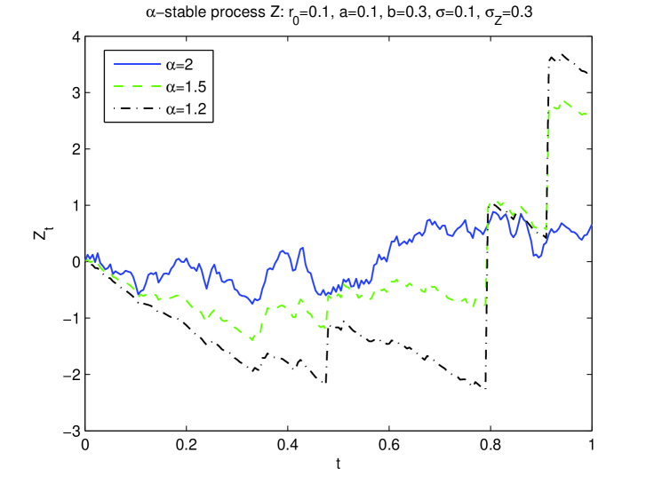
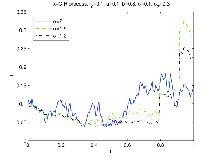
In the first example, we present in Figure 1 a trajectory of the $\alpha$ -stable Lévy process $Z$ for three different values of $\alpha$ : 2, 1.5 and 1.2 respectively. The other parameters are fixed to be $a=0.1$ , $b=0.3$ , $\sigma=0.1$ , $\sigma_{Z}=0.3$ and $r_{0}=0.1$ . We see that smaller values of $\alpha$ imply larger jumps and deeper negative drift between the jumps in the process $Z$ . We then illustrate in Figure 2 the $\alpha$ -CIR process for the short interest rate $r$ described in Definition 2.1, by using the same trajectory of $Z$ as in Figure 1. We observe that since the jumps are related to the actual level of the interest rate, the smaller values of $\alpha$ correspond to a persistency of low interest rate in Figure 2.

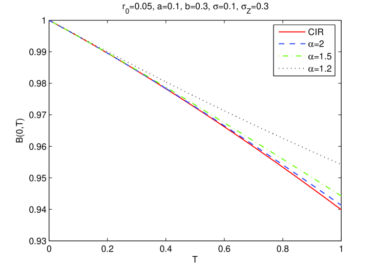
Refer to caption — Figure 1: The $\alpha$ -stable Lévy process $Z$ for different values of $\alpha$ .

In the second example, we show by Figure 3 the sovereign bonds price $B(0,T)$ given in Proposition 4.4. The parameters are $a=0.1$ , $b=0.3$ , $\sigma=0.1$ , $\sigma_{Z}=0.3$ and $r_{0}=0.05$ . Besides the three values of $\alpha$ : 2, 1.5 and 1.2, we also consider the bond price in the classical CIR model (when $\sigma_{Z}=0$ ). It is interesting to note, as already shown in Proposition 4.5, that for a fixed maturity, the bond prices are decreasing with respect to the value of $\alpha$ , with the lowest price in the CIR model. This observation means that smaller $\alpha$ corresponds, in expectation sense, to a lower interest rate phenomenon, even though this case also implies larger positive jumps in the short rate (as in the next figures).

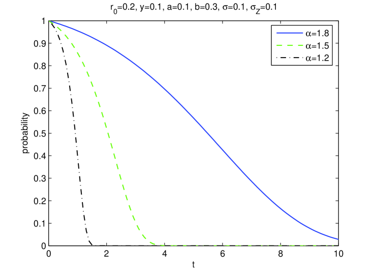
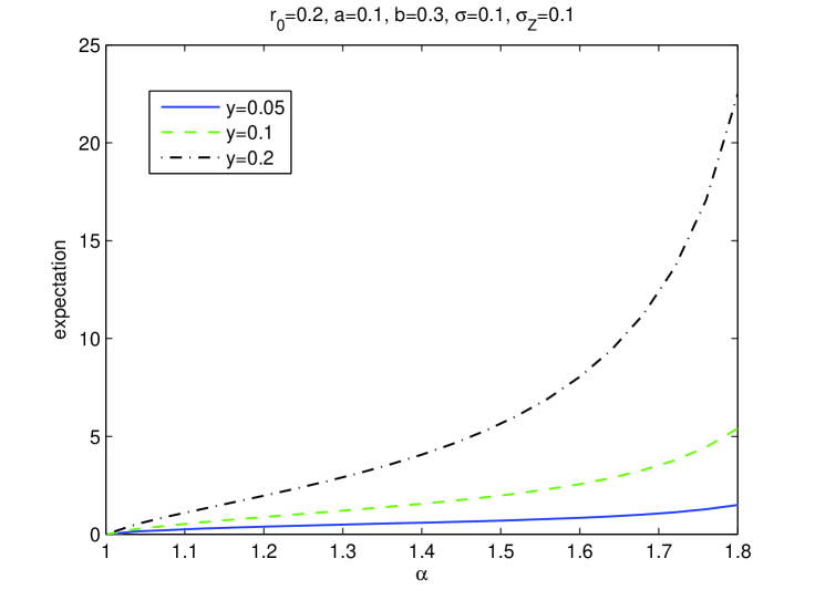
Finally, we illustrate the behaviors of the first large jump $\tau_{\overline{y}}$ (as in (50)) that the short rate process exceeding $\overline{y}$ . The parameters are $a=0.1$ , $b=0.1$ , $\sigma=0.1$ , $\sigma_{Z}=0.1$ , $r_{0}=0.2$ and $y=0.1$ . Figure 4 shows the probability function $\mathbb{P}(\tau_{\overline{y}}>t)$ , given by Corollary 5.2, for different values of $\alpha$ . We see that this probability converges to $0$ very quickly for smaller values of $\alpha$ , and with a much longer time for large values of $\alpha$ . Figure 5 illustrates the expectation of $\tau_{\overline{y}}$ given by Proposition 5.3, as a function of $\alpha$ . The expected jump time is increasing with $\alpha$ , which means that for a smaller $\alpha$ , the first large jump is likely to occur sooner. These two tests show that the $\alpha$ -CIR model with $\alpha<2$ allows to describe the large jumps in the interest rate.

7 Conclusion

The objective of this paper is to introduce the $\alpha$ -CIR short interest rate model, which is an extension of the standard CIR model by adding, besides the Brownian motion, a spectrally positive $\alpha$ -stable Lévy process and preserving the branching property.

Our main financial contribution is to describe in a parsimonious framework a number of well-established and seemingly puzzling facts observed in the current sovereign bond markets. In particular, we reconcile in this relatively simple model the presence of significant variations of the interest rates together with the actual persistency of very low interest rates. Moreover, the evolution of the interest rate in our model exhibits the clustering or self-exciting properties which are recently highlighted in stochastic modelling especially in finance.

An interesting financial result is that the bond price increases with the tail fatness of the jump process which is counter-intuitive and opens the discussion of the consequence on the risk analysis. In particular, our model forecasts that the persistency of very low interest rates is accentuated by this tail fatness and this persistency is statistically broken by the arrival of the first large jump whose expected arrival probability decreases with the rate itself.

The main mathematical contribution is the introduction of a more general integral representation of the $\alpha$ -CIR model by using random fields. This integral representation contributes largely to simplify the mathematical proofs and helps to establish a link of our model to the CBI processes, and then to the affine interest rate models. We also characterize, using this representation, the law of the frequency of large jumps and the law of the first one.

From computational point of view, we show that our model admits closed-form formulae up to numerical integrations for a large class of relevant quantities, for instance for the bond prices and derivatives, and also for the law and the expectation of the first large jump. The perspective of further research work consists of empirical and statistical analysis of the $\alpha$ -CIR interest rate model. The integral representation may also open a range of extensions for other financial modelling.

References

[1] Aït-Sahalia, Y. and Jacod, J. (2009): Estimating the Degree of Activity of Jumps in High Frequency Data. The Annals of Statistics. 37, 2202-2244.
[2] Aït-Sahalia, Y., Cacho-Diaz, J., and Laeven, R. J. (2015): Modeling financial contagion using mutually exciting jump processes. Journal of Financial Economics. 117(3), 585-606.
[3] Albeverio, S., Lytvynov, E. and Mahnig, A. (2004): A model of the term structure of interest rates based on Lévy fields. Stochastic Processes and their Applications, 114:251-263.
[4] Asmussen, S and Rosinski, J. (2001): Approximations of small jumps of Lévy processes with a view towards simulation, Journal of Applied Probability, 38, 482-493.
[5] Barndorff-Nielsen, O.E. and Shephard, N. (2000): Modelling by Lévy Processes for Financial Econometrics, in Lévy Processes Theory and Applications, eds. Barndorff-Nielsen, Mikosch and Resnick, Boston, Birkhauser:
[6] Brown, S. J., and Dybvig, P. H. (1986): The empirical implications of the Cox, Ingersoll, Ross theory of the term structure of interest rates. J. Finance, 617-630.
[7] Cox, J., Ingersoll, J. and Ross, S. (1985): A theory of the term structure of interest rate. Econometrica 53, 385-408.
[8] Dassios, A. and Zhao, H. (2011): A dynamic contagion process, Advances in Applied Probability, 43(3), 814-846.
[9] Dawson, D.A. and Li, Z. (2006): Skew convolution semigroups and affine Markov processes. Ann. Probab. 34, 1103-1142.
[10] Dawson, A and Li, Z. (2012): Stochastic equations, flows and measure-valued processes. Annals of Probability. 40 (2), 813-857.
[11] Duffie, D., Filipović, D. and Schachermayer, W. (2003): Affine processes and applications in finance, Annals of Applied Probability, 13(3), 984-1053.
[12] Duhalde, X., Foucart, C. and Ma, C. (2014): On the hitting times of continuous-state branching processes with immigration, Stochastic Process. Appl. 124(12), 4182-4201.
[13] Eberlein, E. and Raible, S., Term structure models driven by general Lévy processes. Math. Finan. 9: 31-53, 1999.
[14] El Karoui, N. and Méléard, S.: Martingale measures and stochastic calculus. Probab. Theory Related Fields. 84 (1990), 83–101.
[15] Errais, E., Giesecke, K. and Goldberg, L. (2010): Affine Point Processes and Portfolio Credit Risk SIAM Journal on Financial Mathematics, 1, 642-665.
[16] Ethier, S.N. and Kurtz, T.G. (1986): Markov Processes: Characterization and Convergence. John Wiley and Sons, New York.
[17] Filipović, D. (2001): A general characterization of one factor affine term structure models. Finance Stochast. 5, 389-412.
[18] Filipović, D. (2009): Term Structure Models, Springer, New York.
[19] Filipović, D., Tappe, S. and Teichmann, J., (2010) Term structure model driven by Wiener process and Poisson measures: existence and positivity. SIAM Journal on Financial Mathematics, 1(1):523-554.
[20] Foucart, C. and Uribe Bravo, G., (2014): Local extinctions in continuous state branching processes with immigration. Bernoulli. 20 (4), 1819-1844.
[21] Fu, Z. and Li, Z. (2010): Stochastic equations of non-negative processes with jumps. Stochastic Processes and their Applications 120, 306-330.
[22] Gibbons, M. R., and Ramaswamy, K. (1993): A test of the Cox, Ingersoll, and Ross model of the term structure. R. Financial Studies, 6(3), 619-658.
[23] Hawkes, A. G. (1971): Spectra of Some Self-Exciting and Mutually Exciting Point Processes. Biometrika 58, 83-90.
[24] He, X. and Li, Z. (2015): Distributions of jumps in a continuous-state branching process with immigration.(http://math0.bnu.edu.cn/ $\tilde{}$ lizh/research/pdffiles/16distrjum.pdf).
[25] Ikeda, N. and Watanabe, S. (1989): Stochastic Differential Equations and Diffusion Processes. North-Holland/Kodansha, Amsterdam/Tokyo.
[26] Kallsen, J. and Muhle-Karbe, J. (2010), Exponentially affine martingales, affine measure changes and exponential moments of affine processes, Stochastic Processes and their Applications, 120: 163-181.
[27] Kawazu, K. and Watanabe, S. (1971): Branching processes with immigration and related limit theorems. Theory Probab. Appl. 16, 36-54.
[28] Kennedy, D. (1994): The term structure of interest rates as a Gaussian random field. Mathematical Finance 4:247-258.
[29] Jaisson, T., and Rosenbaum, M. (2015): Limit theorems for nearly unstable Hawkes processes. Annals of Applied Probability, 25(2), 600-631.
[30] Li, Z. (2011): Measure-Valued Branching Markov Processes. Springer, Berlin.
[31] Li, Z. and Ma, C. (2008): Catalytic discrete state branching models and related limit theorems. Journal of Theoretical Probability, 21, 936-965.
[32] Li, Z. and Ma, C. (2015): Asymptotic properties of estimators in a stable Cox-Ingersoll-Ross model. Stochastic Process. Appl. 125(8), 3196-3233.
[33] Rambaldi, M., Pennesi, P., and Lillo, F. (2015): Modeling FX market activity around macroeconomic news: a Hawkes process approach. Physical Review E, 91(1), 012819.

Appendix A Constructive proof of Proposition 3.3

Proof. Step 1: branching without immigration. Consider a special case of (2) with $b=0$ and we call it a CB process, i.e. a continuous state branching process without immigration,

\displaystyle r_{t}^{x}=x-a\int_{0}^{t}r_{s}^{x}ds+\sigma\int_{0}^{t}\int_{0}^{r_{s}^{x}}W(ds,du)+\sigma_{Z}\int_{0}^{t}\int_{0}^{r_{s-}^{x}}\int_{\mathbb{R}^{+}}\zeta\widetilde{N}(ds,du,d\zeta),

with initial value $x\geq 0$ . By the proof of Proposition 2.6, $r_{t}^{x}$ is increasing of $x$ . Furthermore, for $x\geq y$ , $r_{t}^{x}-r_{t}^{y}$ is independent of $r_{t}^{y}$ and have the same distribution of $r_{t}^{x-y}$ . Then for any $t$ , $\{r_{t}^{x}:x\geq 0\}$ is a Lévy subordinator. The Lévy-Khintchine Formula implies that

\displaystyle\mathbb{E}[e^{-pr_{t}^{x}}]=e^{-xv(t,p)}

for some Lévy exponent $v(t,p)$ and $v(0,p)=p$ . Since $\{r_{s}^{x}:s\geq 0\}$ is the unique strong solution of the above equation, it is a Markov process, i.e., $E[\exp({-pr_{t+s}^{x}})|\mathcal{F}_{s}]=\exp({r_{s}^{x}v(t,p)})$ , which implies that $v(s,v(t,p))=v(s+t,p)$ . Apply Itô’s formula to $\exp({-pr_{s}^{x}})$ and take the expectation,

\displaystyle e^{-xv(s,p)}-e^{-px}=\Psi(p)\int_{0}^{s}\mathbb{E}[e^{-pr_{u}^{x}}r_{u}^{x}]du.

Fix $t$ . Replace $p$ by $v(t,p)$ in the above equation,

\displaystyle e^{-xv(s+t,p)}-e^{-xv(t,p)}=\Psi(v(t,p))\int_{0}^{s}\mathbb{E}\left[e^{-v(t,p)r_{u}^{x}}r_{u}^{x}\right]du.

Differentiating both sides of the equation w.r.t $s$ at $s=0$ , we have that $\frac{\partial{v(t,p)}}{\partial{t}}=-\Psi(v(t,p))$ .

Step 2: introduction of the auxiliary jump process. Let $c>0$ and let $J_{t}$ be a Poisson process with parameter $\lambda_{J}>0$ independent of $(W,N)$ . Then we define the process $Y$ with initial value $x$ by

\displaystyle Y^{x}_{t}=x+cJ_{t}-a\int_{0}^{t}Y^{x}_{s}ds+\sigma\int_{0}^{t}\int_{0}^{Y^{x}_{s}}W(ds,du)+\sigma_{Z}\int_{0}^{t}\int_{0}^{Y^{x}_{s-}}\int_{\mathbb{R}^{+}}\zeta\widetilde{N}(ds,du,d\zeta).

(65)

Let us assume the following: (a) At $t=0$ there is one individual with mass $x$ . It evolves and gives mass $r_{t}^{x}$ at time $t>0$ . (b) Immigrants with each mass $c$ arrive according to the Poisson process $J_{t}$ . The arrival times of $J_{t}$ is denoted by $0\leq\tau_{1}\leq\cdots\leq\tau_{n}\leq\cdots$ . If one immigrant arrives at time $\tau_{k}$ , it gives mass $r^{(k)}_{t-\tau_{k}}$ at time $t$ , where $r^{(k)}_{\cdot}$ is an independent copy of $r_{\cdot}(c)$ . Then we have that

\displaystyle Y^{x}_{t}=r_{t}^{x}+\sum_{k=1}^{J_{t}}r^{(k)}(t-\tau_{k}).

(66)

We now define a Picard sequence $\widehat{r}^{(k)}_{t}$ by the first step $\widehat{r}^{(0)}_{t}=r_{t}^{x}$ and the relation between $\widehat{r}^{(k-1)}_{t}$ and $\widehat{r}^{(k)}_{t}$ defined as

\displaystyle\widehat{r}^{(k)}_{t}=\widehat{r}^{(k-1)}_{\tau_{k}}+c-a\int_{0}^{t}\widehat{r}^{(k)}_{s}ds+\sigma\int_{0}^{t}\int_{0}^{\widehat{r}^{(k)}_{s}}W^{\tau_{k}}(ds,du)+\sigma_{Z}\int_{0}^{t}\int_{0}^{\widehat{r}^{(k)}_{s-}}\int_{\mathbb{R}^{+}}\zeta\widetilde{N}^{\tau_{k}}(ds,du,d\zeta).

Here $(W^{\tau_{k}},N^{\tau_{k}})$ is the translator of $(W,N)$ at $\tau_{k}$ , i.e. $W^{\tau_{k}}([0,t]\times A)=W([\tau_{k},\tau_{k}+t]\times A)$ and $N^{\tau_{k}}([0,t]\times A\times C)=N([\tau_{k},\tau_{k}+t]\times A\times C)$ . Consider (65), we have easily that $Y_{t}=\widehat{r}^{(0)}_{t}$ for $0\leq t<\tau_{1}$ and similarly $Y_{t}=\widehat{r}^{(1)}_{t-\tau_{1}}$ for $\tau_{1}\leq t<\tau_{2}$ . More generally, applying Proposition 2.6, it is not hard to see that $\overline{r}^{(1)}_{t}:=\widehat{r}^{(1)}_{t}-\widehat{r}^{(0)}_{\tau_{1}+t}$ is independent of $\{\widehat{r}^{(0)}_{t}\}$ and have the same distribution as $\{r_{t}^{c}\}$ . Thus for $\tau_{1}\leq t<\tau_{2}$ , $Y_{t}^{x}=r_{t}^{x}+\overline{r}^{(1)}_{t-\tau_{1}}$ . Similarly, for $\tau_{k-1}\leq t<\tau_{k}$ , $Y_{t}^{x}=r_{t}^{x}+\sum_{i=1}^{k}\overline{r}^{(i)}_{t-\tau_{i}}$ , where $\overline{r}^{(k)}_{t}=\widehat{r}^{(k)}_{t}-\widehat{r}^{(k-1)}_{\tau_{k}-\tau_{k-1}+t}$ . Thus we have (66). Also by Step 1 and the exponential formula,

	$\displaystyle\mathbb{E}\left[e^{-qY^{x}_{t}}\right]$	$\displaystyle=$	$\displaystyle\exp\left\{-xv(t,p)+\lambda_{J}\int_{0}^{t}\left(1-e^{-cv(t-s,p)}\right)ds\right\}$
		$\displaystyle=$	$\displaystyle\exp\left\{-xv(t,p)+\lambda_{J}\int_{0}^{t}\left(1-e^{-cv(u,p)}\right)du\right\}.$

The last equality follows from replacing $t-s$ by $u$ .

Step 3: limit using the renormalization of the auxiliary process. Consider a sequence of $Y^{(n)}$ defined by (65), where $J_{t}$ replaced by $J^{(n)}_{t}$ with parameter $\lambda_{n}=abn$ and $c$ replaced by $c_{n}=1/n$ . Let $r$ given by (2) with initial value $x$ . It is not hard to see that $Y^{(n)}\rightarrow r$ in law as $n\rightarrow\infty$ . Then

\displaystyle\mathbb{E}\left[e^{-pr_{t}}\right]=\lim_{n\rightarrow\infty}\mathbb{E}\left[e^{-pY^{(n)}_{t}}\right]=\exp\left\{-xv(t,p)-ab\int_{0}^{t}v(s,p)ds\right\}

$\Box$