$\alpha$-decay half-lives for even-even isotopes of W to U

In this section, we briefly introduce how the DRHBc includes deformations and pairing correlation. The $\alpha$-decay half-lives in the WKB approximation require density distributions for a daughter nucleus and the $\alpha$-particle. We introduce how the density distributions are described in the DRHBc.

The relativistic mean-field theory is built from the Lagrangian density Ring:1996qi . The Lagrangian density for point-coupling is described in detail in Ref. A_textbook_of_Jie_Meng . The relativistic Hartree-Bogoliubov equation which incorporates the mean-field and pairing field simultaneously is obtained with the variational method and the Bogoliubov transformation Kucharek:1991arbi ,

$$\displaystyle\begin{pmatrix}h_{\rm D}-\lambda_{\tau}&\Delta\\ -\Delta^{*}&-h^{*}_{\rm D}+\lambda_{\tau}\end{pmatrix}\begin{pmatrix}U_{k}\\ V_{k}\end{pmatrix}=E_{k}\,\begin{pmatrix}U_{k}\\ V_{k}\end{pmatrix},$$

(1)

where $h_{\rm D}$ is Dirac Hamiltonian for the nucleons, $\lambda_{\tau}$ represents the Fermi energy of a nucleon, $\Delta$ is the pairing field, $U_{k}$ and $V_{k}$ correspond to the quasiparticle wave functions, and $E_{k}$ means the energy of a quasiparticle state $k$. The pairing potential for particle-particle channel is used

$\displaystyle\Delta_{kk^{{}^{\prime}}}(\bm{r},\bm{r^{{}^{\prime}}})=-\sum_{\tilde{k}\tilde{k}^{{}^{\prime}}}\,V^{pp}_{kk^{{}^{\prime}},\tilde{k}\tilde{k}^{{}^{\prime}}}(\bm{r},\bm{r^{{}^{\prime}}})\kappa_{\tilde{k}\tilde{k}^{{}^{\prime}}}(\bm{r},\bm{r^{{}^{\prime}}}),$

(2)

where, $k$, $k^{{}^{\prime}}$, $\tilde{k}$, and $\tilde{k}^{{}^{\prime}}$ denote the quasiparticle states and the pairing tensor is defined by $\kappa=V^{\ast}U^{T}$ A_textbook_of_Peter_Ring . For pairing interaction in the particle-particle channel $V^{pp}$, in the DRHBc, the density-dependent zero-range pairing interaction is used

$\displaystyle V^{pp}(\bm{r},\bm{r^{{}^{\prime}}})=\frac{V_{0}}{2}\left(1-P^{\sigma}\right)\delta(\bm{r}-\bm{r^{{}^{\prime}}})\left(1-\frac{\rho(\bm{r})}{\rho_{\rm sat}}\right),$

(3)

where $\rho_{\rm sat}$ is the nuclear saturation density. The Dirac Hamiltonian $h_{\rm D}$ for the nucleons is given as A_textbook_of_Jie_Meng

$$h_{\rm D}=\bm{\alpha}\cdot\bm{p}\,+\,\beta\left(M+S(\bm{r})\right)\,+\,V(\bm{r})$$

(4)

where $S(\bm{r})$ and $V(\bm{r})$ are scalar and vector potentials, which are expressed as

	$\displaystyle S(\bm{r})$	$\displaystyle=$	$\displaystyle\alpha_{\rm S}\rho_{\rm S}+\beta_{\rm S}\rho^{2}_{\rm S}+\gamma_{\rm S}\rho^{3}_{\rm S}+\delta_{\rm S}\Delta\rho_{\rm S},$
	$\displaystyle V(\bm{r})$	$\displaystyle=$	$\displaystyle\alpha_{V}\rho_{V}+\gamma_{V}\rho^{3}_{V}+\delta_{V}\Delta\rho_{V}+eA_{0}+\alpha_{\rm TV}\tau_{3}\rho_{\rm TV}+\delta_{\rm TV}\tau_{3}\Delta\rho_{\rm TV}.$		(5)

The local densities $\rho_{\rm S}(\bm{r})$, $\rho_{\rm V}(\bm{r})$, and $\rho_{\rm TV}(\bm{r})$ are represented as

	$\displaystyle\rho_{\rm S}(\bm{r})=\sum_{k>0}\,\bar{V_{k}}(\bm{r})V_{k}(\bm{r}),$
	$\displaystyle\rho_{\rm V}(\bm{r})=\sum_{k>0}\,V^{\dagger}_{k}(\bm{r})V_{k}(\bm{r}),$
	$\displaystyle\rho_{\rm TV}(\bm{r})=\sum_{k>0}\,V^{\dagger}_{k}(\bm{r})\tau_{3}V_{k}(\bm{r}),$		(6)

where the summation for $k$ is performed only in positive energy in Fermi sea with the no-sea approximation. In the DRHBc, spatial reflection symmetry is preserved. Thus, the densities ($\rho_{\rm S}(\bm{r})$, $\rho_{\rm V}(\bm{r})$, $\rho_{\rm TV}(\bm{r})$) are expanded using Legendre polynomials as Price:1987sf

$$\rho(\bm{r})=\sum_{\lambda_{\rm L}}\,\rho_{\lambda_{\rm L}}(r)P_{\lambda_{\rm L}}(\cos\theta).\,\,\,\lambda_{\rm L}=0,\,2,\,4,\,\cdots.$$

(7)

For the DRHBc, as described in Ref. Choi:2022rdj , the pairing strength $V_{0}=-325$ MeV$\cdot{\rm fm}^{3}$ and the angular momentum cutoff for the Dirac Woods-Saxon basis $J_{\rm max}=23/2~{}\hbar$ are taken. Other are described in Ref. DRHBcMassTable:2022uhi .

The $\alpha$-decay process is understood as the formation of $\alpha$-particle inside the parent nucleus and penetrating the potential barrier of the daughter nucleus with a given $Q$-value $Q_{\alpha}$ as in Fig. 1. Therefore, the $\alpha$-decay half-life can be calculated within the WKB approximation as Gurvitz:1986uv ; Xu:2006cr

	$\displaystyle T_{1/2}$	$\displaystyle=$	$\displaystyle\frac{\hbar\ln 2}{\Gamma},$		(8)
	$\displaystyle\Gamma$	$\displaystyle=$	$\displaystyle P_{\alpha}N_{\rm f}\frac{\hbar^{2}}{4\mu}P_{\rm total},$		(9)

where $\Gamma$, $P_{\alpha}$, $N_{\rm f}$, and $P_{\rm total}$ are decay width, preformation factor of $\alpha$-particle, normalization factor for bound-stated wave function, and the total penetration probability, respectively. To calculate the decay width $\Gamma$, the preformation factor $P_{\alpha}$ must be first calculated. However, the preformation factor $P_{\alpha}$ in Eq. (9) cannot yet be calculated microscopically in the DRHBc framework. Instead we calculate $P_{\alpha}$ as in the cluster-formation model SalehAhmed:2013nwa . The preformation factor of $\alpha$-particle $P_{\alpha}$ for even-even nuclei is calculated in the cluster-formation model Ahmed:2015kra ; Deng:2015qha as

$$P_{\alpha}=\frac{2S_{\rm p}+2S_{\rm n}-S_{\alpha}}{S_{\alpha}},$$

(10)

where $S_{\rm p}$, $S_{\rm n}$, $S_{\alpha}$ are one-proton, one-neutron, and $\alpha$-particle separation energies, respectively. Separation energies can be obtained as

	$\displaystyle S_{\rm p}(Z,N)$	$\displaystyle=$	$\displaystyle E_{\rm b}(Z,N)-E_{\rm b}(Z-1,N),$		(11)
	$\displaystyle S_{\rm n}(Z,N)$	$\displaystyle=$	$\displaystyle E_{\rm b}(Z,N)-E_{\rm b}(Z,N-1),$		(12)
	$\displaystyle S_{\alpha}(Z,N)$	$\displaystyle=$	$\displaystyle E_{\rm b}(Z,N)-E_{\rm b}(Z-2,N-2),$		(13)

where $E_{\rm b}(Z,N)$ is the binding energy of given proton number $Z$ and neutron number $N$. We take $E_{\rm b}(Z,N)$ from both AME2020 and the results of the DNN study CK2 since, at the moment, the binding energies for odd-$A$ nuclei are not available in the DRHBc framework. The normalization factor and the total penetration probability for axially deformed nuclei in Eq. (9) are given as

	$\displaystyle N_{\rm f}$	$\displaystyle=$	$\displaystyle\frac{1}{2}\int_{0}^{\pi}N_{\rm f}(\beta)\sin\beta d\beta,$		(14)
	$\displaystyle P_{\rm total}$	$\displaystyle=$	$\displaystyle\frac{1}{2}\int_{0}^{\pi}\exp\bigg{[}-2\int_{r_{2}(\beta)}^{r_{3}(\beta)}k(r^{\prime},\beta)d{r}^{\prime}\bigg{]}\sin\beta d\beta,$		(15)

where the normalization factor $N_{\rm f}(\beta)$ for the orientation angle between the $\alpha$-particle and the symmetry axis of the daughter nucleus $\beta$ and $k(r,\beta)$ are expressed as

	$\displaystyle N_{\rm f}(\beta)$	$\displaystyle=$	$\displaystyle\bigg{[}\int_{r_{1}(\beta)}^{r_{2}(\beta)}\frac{d{r}^{\prime}}{k(r^{\prime},\beta)}\cos^{2}\bigg{(}\int_{r_{1}(\beta)}^{r^{\prime}}d{r}^{\prime\prime}k(r^{\prime\prime},\beta)-\frac{\pi}{4}\bigg{)}\bigg{]}^{-1}\simeq\bigg{[}\int_{r_{1}(\beta)}^{r_{2}(\beta)}\frac{dr^{\prime}}{2k(r^{\prime},\beta)}\bigg{]}^{-1},$		(16)
	$\displaystyle k(r,\beta)$	$\displaystyle=$	$\displaystyle\sqrt{\frac{2\mu}{\hbar^{2}}|Q_{\alpha}-V(r,\beta)|},$		(17)

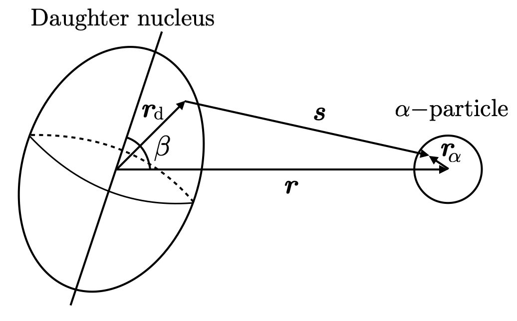
and $\mu$ is the reduced mass of the $\alpha$-particle and daughter nucleus, $r_{1,2,3}(\beta)$ are the classical turning points which are marked in Fig. 1, and $\beta$ is the azimuthal angle between the symmetry axis of daughter nucleus and the direction of the produced $\alpha$-particle as in Fig. 2. Note that the outer turning point $r_{3}$ is determined mostly by the Coulomb potential. We take empirical $Q_{\alpha}^{\rm exp}$ from AME2020 Wang:2021xhn .

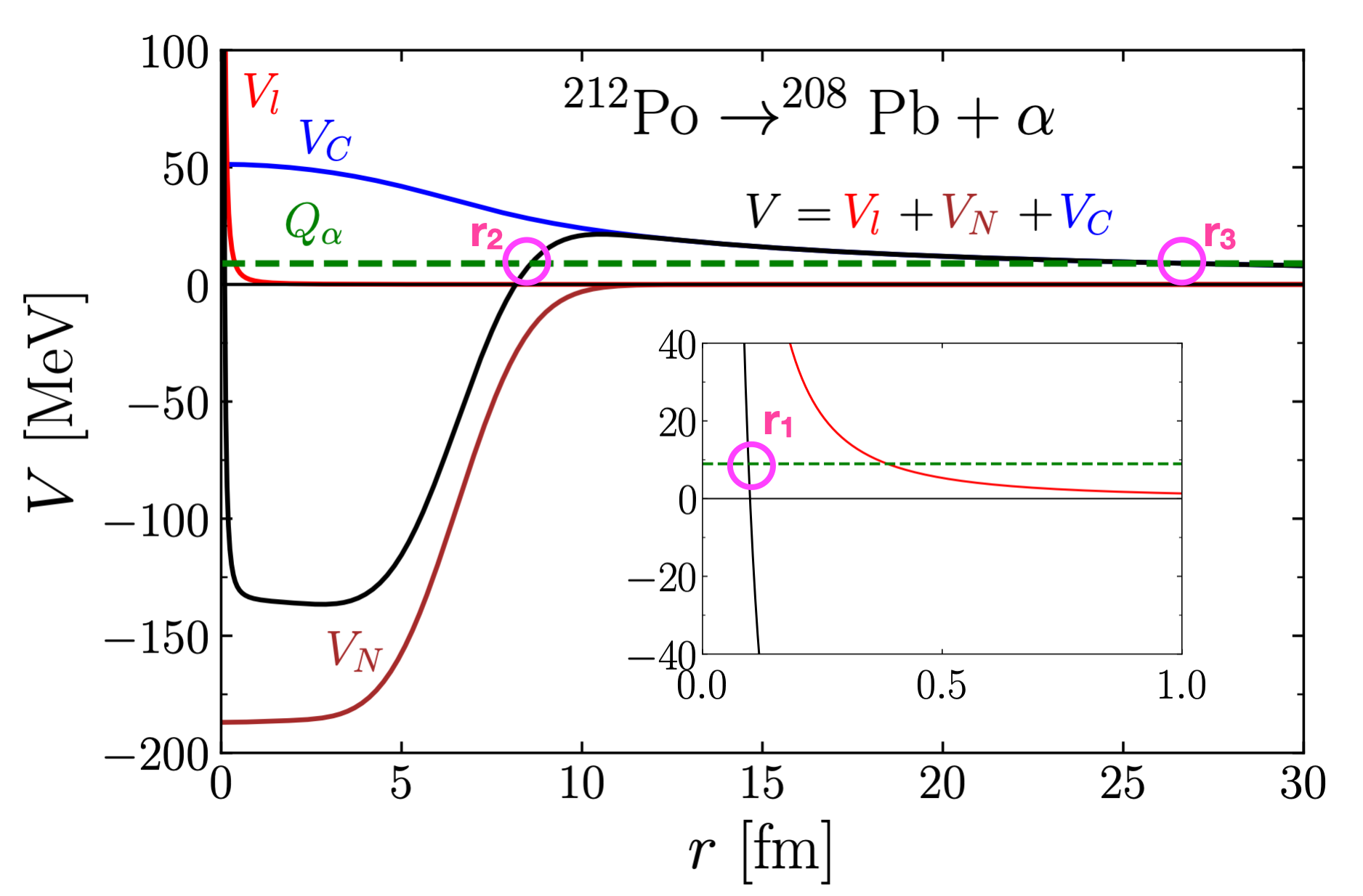
In the density-dependent cluster model, the potential $V(r,\beta)$ consists of centrifugal potential $V_{l}(r)$, nucleus-nucleus double-folding potential $V_{\rm N}(r,\beta)$, and Coulomb potential $V_{\rm C}(r,\beta)$ Wan:2021wny , as plotted in Fig. 1,

$$V(r,\beta)=V_{l}(r)+V_{\rm N}(r,\beta)+V_{\rm C}(r,\beta).$$

(18)

The centrifugal potential is expressed using the Langer modified form Langer:1937qr ; Buck:1992zza ; Buck:1993sku

$$V_{l}(r)=\frac{\hbar^{2}}{2\mu}\frac{(l+1/2)^{2}}{r^{2}},$$

(19)

where $l$ is the quantum number corresponding to the orbital angular momentum transferred by $\alpha$-particle. As we only consider the $\alpha$-decay of even-even nuclei, we apply $l=0$ Xu:2006fq . The nuclear and Coulomb potentials are built from double-folding model Bertsch:1977sg ; Satchler:1979ni ; Kobos:1982pdw ; Kobos:1984zz :

	$\displaystyle V_{\rm N}(r,\beta)$	$\displaystyle=$	$\displaystyle\lambda\int d{\bm{r}}_{\rm d}d{\bm{r}}_{\alpha}\rho_{\rm d}({\bm{r}}_{\rm d})\rho_{\alpha}({\bm{r}}_{\alpha})v({\bm{s}}),$		(20)
	$\displaystyle V_{\rm C}(r,\beta)$	$\displaystyle=$	$\displaystyle\int d{\bm{r}}_{\rm d}d{\bm{r}}_{\alpha}\rho_{\rm d}^{\rm proton}({\bm{r}}_{\rm d})\rho_{\alpha}^{\rm proton}({\bm{r}}_{\alpha})\frac{e^{2}}{s},$		(21)

where we take $e^{2}=1.4399764$ MeV$\cdot$fm and plot ${\bm{s}}={\bm{r}}+{\bm{r}}_{\alpha}-{\bm{r}}_{\rm d}$ in Fig. 2. We set the density distribution of $\alpha$-particle as standard Gaussian form $\rho_{\alpha}(r)=0.4229\exp(-0.7024r^{2})$ Satchler:1979ni . From Eq. (15), it can be seen that $\alpha$-decay half-lives depend largely on the wave number $k(r,\beta)$ in the range of $r=r_{2}\sim r_{3}$. We use the M3Y effective nucleon-nucleon interaction $v({\bf s})$ in MeV unit,

$$v({\bm{s}})=7999e^{-4s}/(4s)-2134e^{-2.5s}/(2.5s)-276(1-0.005Q_{\alpha}/A_{\alpha})\delta({\bm{s}}),$$

(22)

for considering the double-folding potential Bertsch:1977sg ; Kobos:1982pdw . In the above equation, $A_{\alpha}$ is the mass number of $\alpha$-particle and $\delta$ is the delta function.

To calculate $V_{\rm C}$ and $V_{\rm N}$, we use $\rho_{\rm d}$ and $\rho_{\rm d}^{\rm proton}$ calculated from the DRHBc;

$\displaystyle V_{\rm N\ \textrm{or}\ C}(r,\beta)$

$\displaystyle=$

$\displaystyle\sum_{\lambda_{\rm L}=0,2,4,...}V_{{\rm N\ \textrm{or}\ C},\lambda_{\rm L}}(r,\beta).$

(23)

By using the Fourier transformation, one can derive $V_{\rm N,\lambda_{L}}$ and $V_{\rm C,\lambda_{L}}$ as

	$\displaystyle V_{{\rm N},\lambda_{\rm L}}(r,\beta)$	$\displaystyle=$	$\displaystyle\frac{2}{\pi}\int_{0}^{\infty}dkk^{2}j_{\lambda_{\rm L}}(kr)\tilde{\rho}_{\alpha}(k)\bigg{[}\int^{\infty}_{0}dr_{\rm d}r_{\rm d}^{2}\rho_{{\rm d},\lambda_{\rm L}}(r_{\rm d})j_{\lambda_{\rm L}}(kr_{\rm d})\bigg{]}\tilde{v}(k)P_{\lambda_{\rm L}}(\cos\beta),$		(24)
	$\displaystyle V_{{\rm C},\lambda_{\rm L}}(r,\beta)$	$\displaystyle=$	$\displaystyle 8e^{2}\int_{0}^{\infty}dkj_{\lambda_{\rm L}}(kr)\tilde{\rho}_{\alpha}^{\rm proton}(k)\bigg{[}\int^{\infty}_{0}dr_{\rm d}r_{\rm d}^{2}\rho_{{\rm d},\lambda_{\rm L}}^{\rm proton}(r_{\rm d})j_{\lambda_{\rm L}}(kr_{\rm d})\bigg{]}P_{\lambda_{\rm L}}(\cos\beta),$		(25)

where $j_{\lambda_{\rm L}}(kr)$ is the spherical Bessel function. The terms $\tilde{\rho}_{\alpha}(k),\tilde{\rho}_{{\rm d},\lambda_{\rm L}}(k)$, and $\tilde{v}(k)$ are Fourier transformation of $\rho_{\alpha}(r),\rho_{{\rm d},\lambda_{\rm L}}(r)$, and $v(r)$, respectively. The forms of $\tilde{\rho}_{\alpha}(k)$ and $\tilde{v}(k)$ are written in Appendix A of Ref. Bai:2018hbe . The generalized equation is written in Ref. 1983ZPhyA.310..287R . The property $\exp(i{\bm{k}}\cdot{\bm{r}})=\sum_{\lambda_{\rm L}}i^{\lambda_{\rm L}}(2\lambda_{\rm L}+1)j_{\lambda_{\rm L}}(kr)P_{\lambda_{\rm L}}(\cos\theta)$ is used for applying Fourier transformation. We take $\lambda_{\rm L,max}=8$ to be consistent with the current DRHBc results.

In Eq. (20), $\lambda$ is the normalization factor and related to the strength of nuclear potential. It is determined by the Bohr-Sommerfeld quantization condition Xu:2006fq

$$\int_{0}^{\pi}\int_{r_{1}(\beta)}^{r_{2}(\beta)}\sqrt{\frac{2\mu}{\hbar^{2}}[Q_{\alpha}-V(r,\beta)]}\sin\beta drd\beta=(2n+1)\frac{\pi}{2}=(G-L+1)\frac{\pi}{2},$$

(26)

where $r_{1}(\beta),~{}r_{2}(\beta)$ are the set of classical turning points ($Q_{\alpha}=V(r,\beta)$), and $Q_{\alpha}$ and $G$ are the $\alpha$-decay energy and global quantum number, respectively. Note that there is no additional constraint to fix the global quantum number $G$. We take $G$ as follows Buck:1992zz ; Buck:1996zza

	$\displaystyle G=22~{}(N_{\rm par}>126),$
	$\displaystyle G=20~{}(82<N_{\rm par}\leq 126),$

where $N_{\rm par}$ is the neutron number of parent nucleus.

In order to obtain the decay width, in Eq. (9), the preformation factor $P_{\alpha}$ has to be provided. As discussed in the previous section, we calculate $P_{\alpha}$ using binding energies by following the cluster-formation model SalehAhmed:2013nwa as defined in Eq. (10). Since, at the moment, the binding energies for odd-even and odd-odd nuclei are not available in the DRHBc framework, $S_{\rm n}$ and $S_{\rm p}$ cannot be obtained in the DRHBc. Therefore, we use the binding energies obtained from a DNN study CK2 in which available results from the DRHBc calculations and the AME2020 data are used as a training set. When the binding energies are available both in the DRHBc and AME2020, those of AME2020 were used in the training set. To obtain the odd-even and odd-odd binding energies using a deep neural network, the binding energies of even-even and even-odd isotopes from the DRHBc calculations are used as a training set. In addition, to include some information about odd-odd and odd-even isotopes to the deep neural network the authors of  CK2 also use the binding energies in AME2020 Wang:2021xhn as a training set. The inputs of the neutral network are the proton number ($Z$), neutron number ($N$), nuclear pairing ($\delta$) and shell effect ($P$) which are defined by

	$\displaystyle\delta$	$\displaystyle=$	$\displaystyle\frac{(-1)^{Z}+(-1)^{N}}{2},$		(27)
	$\displaystyle P$	$\displaystyle=$	$\displaystyle\frac{\nu_{P}\nu_{n}}{\nu_{P}+\nu_{n}}\,,$		(28)

where $\nu_{P}$ ($\nu_{N}$) is the difference between the proton (neutron) number of an isotope of interest and the nearest magic numbers. For more details of the neutral network to predict the odd-odd and odd-even masses based on the DRHBc and AME2020, we refer to CK2 . For the comparison, we also use the experimental binding energy and $Q_{\alpha}^{\rm exp}$ from AME2020 Wang:2021xhn . Binding energies used in this work are summarized in Tables 1 and 2.

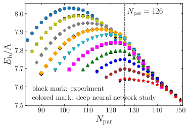
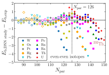
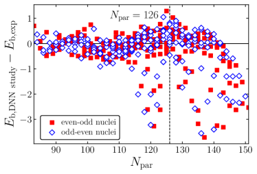
Figure 3 (a) summarizes the binding energy per nucleon for the selected even-even nuclei obtained by the DNN study. For the comparison, experimental binding energies Wang:2021xhn are plotted with black color. In Fig. 3 (b), differences in the binding energies between the DNN study and experimental results are given as a function of the parent neutron number. For nuclei with small neutron number ($N_{\rm par}<126$), the differences between the DNN study and experiment are small compared to nuclei with large neutron number ($N_{\rm par}\geq 126$). This may indicate that DNN study results are more consistent with experiment values for the nuclei with $N_{\rm par}<$ 126. In Fig. 3 (c), the differences in the binding energies between the DNN study and experimental results are summarized as a function of quadrupole deformation $\beta_{2,\rm par}$. This figure shows no strong correlation between the binding energy of the DNN study and the deformation. In Fig. 3 (d), the differences for even-odd and odd-even nuclei are summarized. Overall, it shows similar behavior as even-even nuclei in Fig. 3 (b), but the deviations of the DNN study results from experimental values for even-odd nuclei are relatively larger than those for odd-even nuclei. It may indicate that the DNN study is more sensitive to neutron distributions than proton distributions.

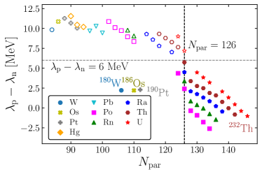
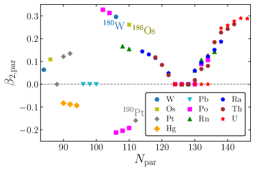
Figure 4 shows the Fermi energy differences and deformation parameters in the DRHBc. The Fermi energy differences are larger than 6 MeV for most of nuclei with $N_{\rm par}<126$ except for ¹⁸⁰W, ¹⁸⁶Os, ¹⁹⁰Pt, and ²⁰⁸Po as in Fig. 4. The experimental $\alpha$-decay half-lives of ¹⁸⁰W, ¹⁸⁶Os, and ¹⁹⁰Pt are important because the half-lives of nearby nuclei are dominated by other decay modes, such as $\beta$-decay. The $\alpha$-decay half-lives of ¹⁸⁰W, ¹⁸⁶Os, and ¹⁹⁰Pt are longest in this study ($10^{25.7}$, $10^{22.8}$, and $10^{19.183}$ s, respectively). These nuclei can be used for verifying whether the half-life calculation provides consistent results for long experimental $\alpha$-decay half-lives. Also, these nuclei can be used to verify whether the half-life for defomed nuclei is accurate since quadrupole deformations of these nuclei are $\beta_{2,\rm par}=0.243$ for ¹⁸⁰W, $\beta_{2,\rm par}=0.209$ for ¹⁸⁶Os, and $\beta_{2,\rm par}=0.163$ for ¹⁹⁰Pt, respectively Moller:2015fba . The relation, $|\beta_{2,\rm par}|$ for ¹⁸⁰W $>$ $|\beta_{2,\rm par}|$ for ¹⁸⁶Os $>$ $|\beta_{2,\rm par}|$ for ¹⁹⁰Pt, can also be confirmed in Fig. 5. In this figure, one can confirm $\beta_{2,{\rm par}}=0.0$ for the nuclei with neutron magic number $N_{\rm par}=126$.

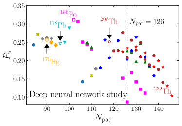
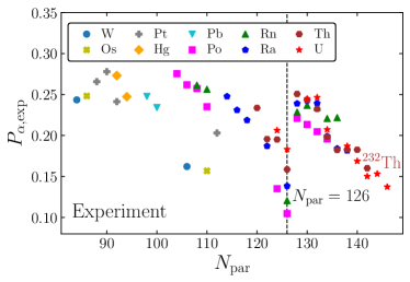
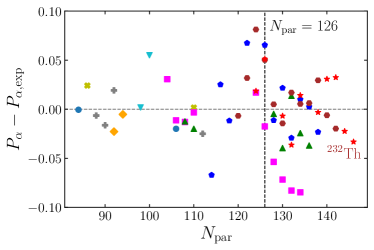
In Fig. 6 (a) and (b), preformation factors obtained with the DNN study CK2 and experimental data (AME2020) are summarized. In Fig. 6 (a), nuclei with empty marks (¹⁷⁰Hg, ¹⁷⁸Pb, ¹⁸⁶Po, ²⁰⁸Th) correspond to the nuclei for which experimental results are not enough to obtain $P_{\alpha}$. Note that binding energies for ¹⁶⁹Hg, ¹⁷⁷Pb, ¹⁸⁵Po, and ²⁰⁷Th are missing in AME2020. In Fig. 6 (b), $P_{\alpha}$ are relatively small at the magic number $N_{\rm par}=126$ and increase as neutron number increases to $N_{\rm par}=128$, independently of nuclei; i.e., $P_{\alpha,{\rm exp}}(N_{\rm p}=128)>P_{\alpha,\rm exp}(N_{\rm p}=126)$. Results with AME2012 also show the similar behavior Deng:2015qha . Except Rn, such a trend exists for the result of the DNN study as in Fig. 6 (a). The differences between the DNN study and experimental results are summarized in Fig. 6 (c). In this figure, below the neutron magic number of parent nuclei $N_{\rm par}=126$, ^202,210Ra isotopes show the largest $P_{\alpha}$ diffenrece in the isotopes. For the magic number $N_{\rm par}=126$, ²¹⁰Po shows smallest preformation factor in the DNN study and experiment. Above the magic number, ^214,216,218Po give largest differences in $P_{\alpha}$. If one compare Fig. 6 with Figs. 4 and 5, there are no direct correlations between $P_{\alpha}$ and the properties of nuclei, such as the Fermi energy difference and the deformation parameter $\beta_{2,{\rm par}}$.

In this section, we present our calculated $\alpha$-decay half-lives with given preformation factors as discussed in the previous section. In order to assess the quality of our results, we use experimental binding energy and $Q_{\alpha}^{\rm exp}$ from AME2020 Wang:2021xhn . For the comparison with experiment, we take the experimental $\alpha$-decay half-lives from NUASE2020 Kondev:2021lzi . Because several decay modes can exist for each nucleus, we consider only 67 experimental data for which the branching ratio of $\alpha$-decay are greater than 99%. The calculated $\alpha$-decay half-lives are also summarized in Tables 1 and 2.

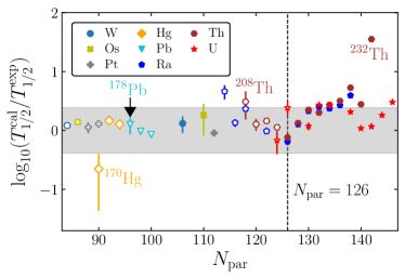
In Fig. 7, our calculated $\alpha$-decay half-lives are compared with experimental values. In order to compare our calculated $\alpha$-decay half-lives with experimental data, we evaluate the standard deviation $\sigma$,

$$\sigma=\sqrt{\frac{1}{N}\sum_{i=1}^{N}\left(\log_{10}T_{1/2,i}^{\rm cal}-\log_{10}T_{1/2,i}^{\rm exp}\right)^{2}},$$

(29)

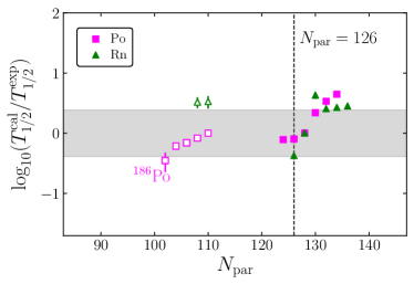
which are plotted as horizontal shaded regions in Fig. 7. Overall, considering the uncertainties in the binding energy estimations by the DNN study, our calculated $\alpha$-decay half lives are consistent with the experimental values within $\pm\sigma$. If we compare Fig. 7 with Fig. 5, the calculated $\alpha$-decay half lives are consistent with experimental values independently of deformation parameter $\beta_{2,{\rm par}}$. Below the neutron magic number $N_{\rm par}=126$, ¹⁷⁰Hg, ¹⁸⁶Po, ²⁰²Ra, and ²⁰⁸Th lie out of the shaded region. The reason for this stems partly from limitation in $P_{\alpha}$ calculations. Note that $P_{\alpha,{\rm exp}}$ for ¹⁷⁰Hg, ¹⁸⁶Po, and ²⁰⁸Th are not available because binding energies for ¹⁶⁹Hg, ¹⁸⁵Po, and ²⁰⁷Th are not available in AME2020. In the DRHBc, $\lambda_{\rm p}>0$ for ¹⁷⁰Hg, ¹⁸⁶Po, and ²⁰⁸Th, it may be more difficult to measure the binding energies of ¹⁶⁹Hg, ¹⁸⁵Po, and ²⁰⁸Th. The predictions from theoretical models such as the DRHBc will be important to study such nuclei. The discrepancy in the $\alpha$-decay half-life of ²⁰²Ra is partly because $P_{\alpha}<P_{\alpha,{\rm exp}}$. Incorrectly estimated $P_{\alpha}$ is not the only cause of discrepancies in the half-lives. For example, the difference in preformation factor of ²¹⁰Ra is large, but the half-life comparison result is very accurate. Beyond the neutron magic number of $130<N_{\rm par}$ for Ra and Th isotopes, the predicted $\alpha$-decay half-lives exceed experimental values, as shown in Fig. 7 (a). This mismatch can be hardly explained by overestimated $P_{\alpha}$ and further study needs to be conducted. For $130<N_{\rm par}<136$ of Po and Rn isotopes (see Fig. 7 (b)), our calculated $\alpha$-decay half-lives are larger than experimental values. This is partly because our estimated $P_{\alpha}$ is smaller than the experimental value as in Fig. 6.

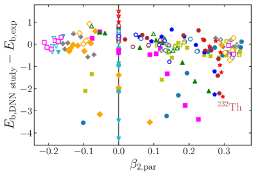
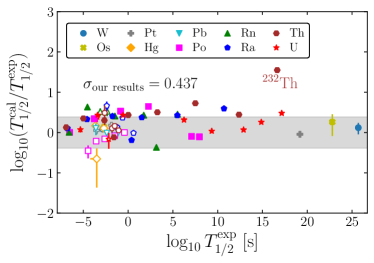
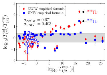
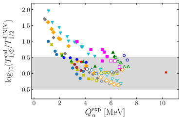
In Fig. 8, the comparion of our calculated $\alpha$-decay half-lives with the experimental $\alpha$-decay results (AME2020) is shown as function of the experimental $\alpha$-decay results. In addition, the comparison of the results with empirical formulae, ZZCW Zhang:2017pwm and UNIV Poenaru:2011zz with the experimental $\alpha$-decay results is also presented as function of the experimental $\alpha$-decay results. The details of the empirical formulae are summarized in the Appendix and results from our study with DNN and empirical formulae are summarized in Tables 3 and 4. In Fig. 8 (b) $\sigma_{\rm ZZCW}$ = 0.671 and $\sigma_{\rm UNIV}$ = 0.403 which are comparable to $\sigma=0.437$ for our DRHBc$+$DNN study calculation. If we consider only proton-rich nuclei (empty marks in Fig. 8), $\sigma_{\rm DRHBc+DNNstudy}=0.405$ and $\sigma_{\rm UNIV}$ = 0.467. This may indicate that DRHBc$+$DNN study is reasonably consistent with experiment for both stable and proton-rich nuclei. ²³²Th, the most stable isotope of Th, is exceptional because the estimated $\alpha$-decay half-lives by empirical formulae as well as our method are much larger than experiment. Further study is required to investigate this largest discrepancy. Based on these observations, we extend our study to the nuclei whose $\alpha$-decay half-lives are not measured experimentally.

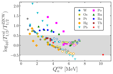
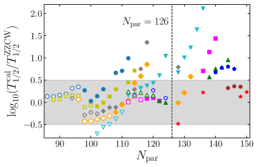
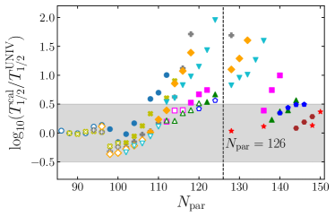
In Fig. 9, we compare our predicted $\alpha$-decay half-lives with empirical formulae results for the nuclei whose $\alpha$-decay half-lives are not available in experiments. The differences between our prediction and empirical formulae become significant as $Q_{\alpha}$ decreases. The difference is significant in the range roughly $110<N_{\rm par}<140$ mainly due to small $Q_{\alpha}$. Note that our calcultions are consistent with empirical formulae results within $\pm 0.7$ for Ra, Th, and U isotopes. For Pb isotopes, the differences between our results and the empirical formulae tends to be more apparent.

References

- (1) O. Kamigaito et al., in 22nd International Conference on Cyclotrons and their Applications (CYC2019) p. MOB01.
- (2) C. Davide, Nature 605, 10.1038/d41586-022-00711-5 (2022).
- (3) X. Zhou and J. Yang, AAPPS Bulletin 32 (2022).
- (4) C. Sturm, B. Sharkov, and H. Stöcker, Nucl. Phys. A 834, 682c (2010).
- (5) S. Jeong, P. Papakonstantinou, H. Ishiyama, and Y. Kim, J. Korean Phys. Soc. 73, 516 (2018).
- (6) B. Buck, A. C. Merchant, and S. M. Perez, Phys. Rev. C 45, 2247 (1992).
- (7) J.-G. Deng, J.-C. Zhao, D. Xiang, and X.-H. Li, Phys. Rev. C 96, 024318 (2017).
- (8) X.-D. Sun, J.-G. Deng, D. Xiang, P. Guo, and X.-H. Li, Phys. Rev. C 95, 044303 (2017).
- (9) C. Xu and Z. Ren, Nucl. Phys. A 760, 303 (2005).
- (10) C. Xu and Z. Ren, Nucl. Phys. A 753, 174 (2005).
- (11) M. Ismail, A. Y. Ellithi, M. M. Botros, and A. Adel, Phys. Rev. C 81, 024602 (2010).
- (12) D. Ni and Z. Ren, Phys. Rev. C 81, 024315 (2010).
- (13) A. Coban, O. Bayrak, A. Soylu, and I. Boztosun, Phys. Rev. C 85, 044324 (2012).
- (14) N. Maroufi, V. Dehghani, and S. A. Alavi, Nucl. Phys. A 983, 77 (2019).
- (15) D. F. Rojas-Gamboa, J. E. P. Velasquez, N. G. Kelkar, and N. J. Upadhyay, Phys. Rev. C 105, 034311 (2022).
- (16) Z. Wang and Z. Ren, Phys. Rev. C 106, 024311 (2022).
- (17) S.-G. Zhou, J. Meng, P. Ring, and E.-G. Zhao, Phys. Rev. C 82, 011301 (2010).
- (18) L. Li, J. Meng, P. Ring, E.-G. Zhao, and S.-G. Zhou, Phys. Rev. C 85, 024312 (2012).
- (19) J. Meng and S. G. Zhou, J. Phys. G 42, 093101 (2015).
- (20) K. Zhang et al., Phys. Rev. C 102, 024314 (2020).
- (21) K. Zhang et al., Atom. Data Nucl. Data Tabl. 144, 101488 (2022).
- (22) C. Pan et al., Phys. Rev. C 106, 014316 (2022).
- (23) E. Teran, V. E. Oberacker, and A. S. Umar, Phys. Rev. C 67, 064314 (2003).
- (24) D. Vretenar, A. V. Afanasjev, G. A. Lalazissis, and P. Ring, Phys. Rept. 409, 101 (2005).
- (25) X.-X. Sun and S.-G. Zhou, Phys. Rev. C 104, 064319 (2021).
- (26) X.-X. Sun and S.-G. Zhou, Sci. Bull. 66, 2072 (2021).
- (27) X. Sun and J. Meng, Phys. Rev. C 105, 044312 (2022).
- (28) W. Sun et al., Chin. Phys. C 46, 064103 (2022).
- (29) W.-h. Long, J. Meng, N. Van Giai, and S.-G. Zhou, Phys. Rev. C 69, 034319 (2004).
- (30) P. Zhao, Z. Li, J. Yao, and J. Meng, Phys. Rev. C 82, 054319 (2010).
- (31) X.-X. Sun, J. Zhao, and S.-G. Zhou, Phys. Lett. B 785, 530 (2018).
- (32) X.-X. Sun, J. Zhao, and S.-G. Zhou, Nucl. Phys. A 1003, 122011 (2020).
- (33) E. J. In, Y. Kim, P. Papakonstantinou, and S.-W. Hong, Int. J. Mod. Phys. E 30, 2150009 (2021).
- (34) K. Zhang et al., Phys. Rev. C 104, 021301 (2021).
- (35) C. Pan et al., Phys. Rev. C 104, 024331 (2021).
- (36) X.-T. He, C. Wang, K.-Y. Zhang, and C.-W. Shen, Chin. Phys. C 45, 101001 (2021).
- (37) Y.-B. Choi, C.-H. Lee, M.-H. Mun, and Y. Kim, Phys. Rev. C 105, 024306 (2022).
- (38) S. Kim, M.-H. Mun, M.-K. Cheoun, and E. Ha, Phys. Rev. C 105, 034340 (2022).
- (39) S. M. Saleh Ahmed, R. Yahaya, S. Radiman, and M. Samudi Yasir, J. Phys. G 40, 065105 (2013).
- (40) S. M. S. Ahmed et al., Eur. Phys. J. A 51, 13 (2015).
- (41) K. Varga, R. G. Lovas, and R. J. Liotta, Phys. Rev. Lett. 69, 37 (1992).
- (42) D. Deng, Z. Ren, D. Ni, and Y. Qian, J. Phys. G 42, 075106 (2015).
- (43) D. Deng and Z. Ren, Phys. Rev. C 93, 044326 (2016).
- (44) N. Wan and J. Fan, Phys. Rev. C 104, 064320 (2021).
- (45) S.-C. Choi, K. Kim, and Y. Kim, Deep learning for nuclear masses in deformed relativistic hartree-bogoliubov theory in continuum, in preparation.
- (46) P. Ring, Prog. Part. Nucl. Phys. 37, 193 (1996).
- (47) J. Meng, Relativistic Density Functional for Nuclear Structure, (World Scientific, Singapore, 2016).
- (48) H. Kucharek and P. Ring, Hadrons and Nuclei 339, 23 (1991).
- (49) P. Ring and P. Schuck, The Nuclear Many-body Problem, (Springer, Heidelberg 1980).
- (50) C. Price and G. Walker, Phys. Rev. C 36, 354 (1987).
- (51) S. A. Gurvitz and G. Kaelbermann, Phys. Rev. Lett. 59, 262 (1987).
- (52) C. Xu, Z. Ren, and Z. Ren, Phys. Rev. C 73, 041301 (2006).
- (53) M. Wang, W. J. Huang, F. G. Kondev, G. Audi, and S. Naimi, Chin. Phys. C 45, 030003 (2021).
- (54) R. E. Langer, Phys. Rev. 51, 669 (1937).
- (55) B. Buck, A. C. Merchant, and S. M. Perez, Phys. Rev. C 45, 1688 (1992).
- (56) B. Buck, A. C. Merchant, and S. M. Perez, Atom. Data Nucl. Data Tabl. 54, 53 (1993).
- (57) C. Xu and Z. Ren, Phys. Rev. C 74, 014304 (2006).
- (58) G. Bertsch, J. Borysowicz, H. McManus, and W. G. Love, Nucl. Phys. A 284, 399 (1977).
- (59) G. R. Satchler and W. G. Love, Phys. Rept. 55, 183 (1979).
- (60) A. M. Kobos, B. A. Brown, P. E. Hodgson, G. R. Satchler, and A. Budzanowski, Nucl. Phys. A 384, 65 (1982).
- (61) A. M. Kobos, B. A. Brown, R. Lindsay, and G. R. Satchler, Nucl. Phys. A 425, 205 (1984).
- (62) D. Bai and Z. Ren, Chin. Phys. C 42, 124102 (2018).
- (63) M. J. Rhoades-Brown, V. E. Oberacker, M. Seiwert, and W. Greiner, Z. Phys. 310, 287 (1983).
- (64) B. Buck, J. C. Johnston, A. C. Merchant, and S. M. Perez, Phys. Rev. C 53, 2841 (1996).
- (65) P. Möller, A. J. Sierk, T. Ichikawa, and H. Sagawa, Atom. Data Nucl. Data Tabl. 109-110, 1 (2016).
- (66) F. G. Kondev, M. Wang, W. J. Huang, S. Naimi, and G. Audi, Chin. Phys. C 45, 030001 (2021).
- (67) S. Zhang, Y. Zhang, J. Cui, and Y. Wang, Phys. Rev. C 95, 014311 (2017).
- (68) D. N. Poenaru, R. A. Gherghescu, and W. Greiner, Phys. Rev. C 83, 014601 (2011).
- (69) B. Sahu, R. Paira, and B. Rath, Nucl. Phys. A 908, 40 (2013).
- (70) D. T. Akrawy and D. N. Poenaru, J. Phys. G 44, 105105 (2017).