This paper was converted on www.awesomepapers.org from LaTeX by an anonymous user.
Want to know more? Visit the Converter page.

α\alpha-Divergence Loss Function for Neural Density Ratio Estimation

Yoshiaki Kitazawa
NTT DATA Mathematical Systems Inc.
Data Mining Division
1F Shinanomachi Rengakan, 35, Shinanomachi
Shinjuku-ku, Tokyo, 160-0016, Japan
kitazawa@msi.co.jp
Abstract

Density ratio estimation (DRE) is a fundamental machine learning technique for capturing relationships between two probability distributions. State-of-the-art DRE methods estimate the density ratio using neural networks trained with loss functions derived from variational representations of ff-divergences. However, existing methods face optimization challenges, such as overfitting due to lower-unbounded loss functions, biased mini-batch gradients, vanishing training loss gradients, and high sample requirements for Kullback–Leibler (KL) divergence loss functions. To address these issues, we focus on α\alpha-divergence, which provides a suitable variational representation of ff-divergence. Subsequently, a novel loss function for DRE, the α\alpha-divergence loss function (α\alpha-Div), is derived. α\alpha-Div is concise but offers stable and effective optimization for DRE. The boundedness of α\alpha-divergence provides the potential for successful DRE with data exhibiting high KL-divergence. Our numerical experiments demonstrate the effectiveness of α\alpha-Div in optimization. However, the experiments also show that the proposed loss function offers no significant advantage over the KL-divergence loss function in terms of RMSE for DRE. This indicates that the accuracy of DRE is primarily determined by the amount of KL-divergence in the data and is less dependent on α\alpha-divergence.

1 Introduction

Density ratio estimation (DRE), a fundamental technique in various machine learning domains, estimates the density ratio r(𝐱)=q(𝐱)/p(𝐱)r^{*}(\mathbf{x})=q(\mathbf{x})/p(\mathbf{x}) between two probability densities using two sample sets drawn separately from pp and qq. Several machine learning methods, including generative modeling [9, 23, 35], mutual information estimation and representation learning [3, 11], energy-based modeling [10], and covariate shift and domain adaptation [29, 12], involve problems where DRE is applicable. Given its potential to enhance a wide range of machine learning methods, the development of effective DRE techniques has garnered significant attention.

Recently, neural network-based methods for DRE have achieved state-of-the-art results. These methods train neural networks as density ratio functions using loss functions derived from variational representations of ff-divergences [22], which are equivalent to density-ratio matching under Bregman divergence [34]. The optimal function for a variational representation of ff-divergence, through the Legendre transform, corresponds to the density ratio.

However, existing neural network methods suffer from several issues. First, an overfitting phenomenon, termed train-loss hacking by Kato and Teshima [14], occurs during optimization when lower-unbounded loss functions are used. Second, the gradients of loss functions over mini-batch samples provide biased estimates of the full gradient when using standard loss functions derived directly from the variational representation of ff-divergence [3]. Third, loss function gradients can vanish when the estimated probability ratios approach zero or infinity [2]. Finally, optimization with a Kullback–Leibler (KL) divergence loss function often fails on high KL-divergence data because the sample requirement for optimization increases exponentially with the true amount of KL-divergence [26, 31, 19].

To address these problems, this study focuses on α\alpha-divergence, a subgroup of ff-divergences, which has a sample complexity independent of its ground truth value. We then present a Gibbs density representation for a variational form of the divergence to obtain unbiased mini-batch gradients, from which we derive a novel loss function for DRE, referred to as the α\alpha-divergence loss function (α\alpha-Div). Despite its simplicity, α\alpha-Div offers stable and effective optimization for DRE.

Furthermore, this study provides technical justifications for the proposed loss function. α\alpha-Div has a sample complexity that is independent of the ground truth value of α\alpha-divergence and provides unbiased mini-batch gradients of training losses. Additionally, choosing α\alpha within the interval (0,1](0,1] ensures that α\alpha-Div remains lower-bounded, preventing train-loss hacking during optimization. By selecting α\alpha from this interval, we also avoid vanishing gradients in neural networks when they reach extreme local minima. We empirically validate our approach through numerical experiments using toy datasets, which demonstrate the stability and efficiency of the proposed loss function during optimization.

However, we observe that the root mean squared error (RMSE) of the estimated density ratios increases significantly for data with higher KL-divergence when using the proposed loss function. The same phenomenon is observed with the KL-divergence loss function. These results suggest that the accuracy of DRE is primarily determined by the magnitude of KL-divergence inherent in the data, rather than by the specific choice of α\alpha in the α\alpha-divergence loss function. This observation highlights a fundamental limitation shared across different ff-divergence-based DRE methods, emphasizing the need to consider the intrinsic KL-divergence of data when evaluating and interpreting DRE performance.

The key contributions of this study are as follows: First, we propose a novel loss function for DRE, termed α\alpha-Div, providing a concise solution to instability and biased gradient issues present in existing ff-divergence-based loss functions. Second, technical justifications and theoretical insights supporting the proposed α\alpha-Div loss function are presented. Third, we empirically confirm the stability and efficiency of the proposed method through numerical experiments. Finally, our empirical results reveal that the accuracy of DRE, measured by RMSE, is primarily influenced by the magnitude of KL-divergence inherent in the data, rather than by the specific choice of α\alpha in the α\alpha-divergence loss function.

2 Problem Setup

Problem definition. PP and QQ are probability distributions on Ωd\Omega\subset\mathbb{R}^{d} with unknown probability densities pp and qq, respectively. We assume p(𝐱)>0q(𝐱)>0p(\mathbf{x})>0\Leftrightarrow q(\mathbf{x})>0 almost everywhere 𝐱Ω\mathbf{x}\in\Omega, ensuring that the density ratio is well-defined on their common support.

The goal of DRE is to accurately estimate r(𝐱)=q(𝐱)/p(𝐱)r^{*}(\mathbf{x})=q(\mathbf{x})/p(\mathbf{x}) from given i.i.d. samples 𝐗^P[R]={𝐱ip}i=1Rp\hat{\mathbf{X}}_{P[R]}=\{\mathbf{x}_{i}^{p}\}_{i=1}^{R}\sim p and 𝐗^Q[S]={𝐱iq}i=1Sq\hat{\mathbf{X}}_{Q[S]}=\{\mathbf{x}_{i}^{q}\}_{i=1}^{S}\sim q.

Additional notation. EP[]E_{P}[\cdot] denotes the expectation under the distribution PP: EP[ϕ(𝐱)]=Ωϕ(𝐱)𝑑P(𝐱)E_{P}[\phi(\mathbf{x})]=\int_{\Omega}\phi(\mathbf{x})dP(\mathbf{x}), where ϕ(𝐱)\phi(\mathbf{x}) is a measurable function over Ω\Omega. E^P[R][]\hat{E}_{P[R]}[\cdot] denotes the empirical expectation of 𝐗^P[R]\hat{\mathbf{X}}_{P[R]}: E^P[R][ϕ(𝐱)]=i=1Rϕ(𝐱ip)/R\hat{E}_{P[R]}[\phi(\mathbf{x})]=\sum_{i=1}^{R}\phi(\mathbf{x}_{i}^{p})/R. The variables in a function or the superscript variable “[R][R]” of E^P[R]\hat{E}_{P[R]} can be omitted when unnecessary and instead represented as EP[ϕ]E_{P}[\phi] or E^P[ϕ]\hat{E}_{P}[\phi]. I(cond)I(\text{cond}) denotes the indicator function: I(cond)=1I(\text{cond})=1 if “cond” is true, and 0 otherwise. Similarly, notations EQ[]E_{Q}[\cdot] and E^Q[S][]\hat{E}_{Q[S]}[\cdot] are defined. E[]E[\cdot] is written for EP[EQ[]]E_{P}[E_{Q}[\cdot]].

3 DRE via ff-divergence variational representations and its major problems

In this section, we introduce DRE using ff-divergence variational representations and ff-divergence loss functions. First, we review the definition of ff-divergences. Next, we identify four major issues with existing ff-divergence loss functions: the overfitting problem with lower-unbounded loss functions, biased mini-batch gradients, vanishing training loss gradients, and high sample requirements for Kullback–Leibler (KL) divergence loss functions.

3.1 DRE via ff-divergence variational representation

First, we review the definition of ff-divergences.

Definition 3.1 (ff-divergence).

The ff-divergence DfD_{f} between two probability measures PP and QQ, which is induced by a convex function ff satisfying f(1)=0f(1)=0, is defined as Df(Q||P)=EP[f(q(𝐱)/p(𝐱))]D_{f}(Q||P)=E_{P}[f(q(\mathbf{x})/p(\mathbf{x}))].

Many divergences are specific cases obtained by selecting a suitable generator function ff. For example, f(u)=uloguf(u)=u\cdot\log u corresponds to KL-divergence.

Then, we derive the variational representations of ff-divergences using the Legendre transform of the convex conjugate of a twice differentiable convex function ff, f(ψ)=supu{ψuf(u)}f^{*}(\psi)=\sup_{u\in\mathbb{R}}\{\psi\cdot u-f(u)\} [21]:

Df(Q||P)=supϕ0{EQ[f(ϕ)]EP[f(f(ϕ))]},D_{f}(Q||P)=\sup_{\phi\geq 0}\Big{\{}E_{Q}\big{[}f^{\prime}(\phi)\big{]}-E_{P}\big{[}f^{*}(f^{\prime}(\phi))\big{]}\Big{\}}, (1)

where the supremum is taken over all measurable functions ϕ:Ω\phi:\Omega\rightarrow\mathbb{R} with EQ[|f(ϕ)|]<E_{Q}[\,|f^{\prime}(\phi)|\,]<\infty and EP[|f(f(ϕ))|]<E_{P}[\,|f^{*}(f^{\prime}(\phi))|\,]<\infty. The maximum value is achieved at ϕ(𝐱)=q(𝐱)/p(𝐱)\phi(\mathbf{x})=q(\mathbf{x})/p(\mathbf{x}).

By replacing ϕ\phi with a neural network model ϕθ\phi_{\theta}, the optimal function for Equation (1) is trained through back-propagation using an ff-divergence loss function, such that

f(R,S)(ϕθ)={E^Q[S][f(ϕθ)]E^P[R][f(f(ϕθ))]},\mathcal{L}_{f}^{(R,S)}(\phi_{\theta})=-\left\{\hat{E}_{Q[S]}\big{[}f^{\prime}(\phi_{\theta})\big{]}-\hat{E}_{P[R]}\big{[}f^{*}(f^{\prime}(\phi_{\theta}))\big{]}\right\}, (2)

where ϕθ\phi_{\theta} is a real-valued function, the superscript variable “(R,S)(R,S)” can be omitted when unnecessary and instead represented as f()\mathcal{L}_{f}(\cdot). As shown in Table 2, we list pairs of convex functions and the corresponding loss functions f(ϕθ)\mathcal{L}_{f}(\phi_{\theta}) in Equation (2) for several ff-divergences.

3.2 Train-loss hacking problem

When ff-divergence loss functions f(ϕθ)\mathcal{L}_{f}(\phi_{\theta}), as defined in Equation (2), are not lower-bounded, overfitting can occur during optimization. For example, we observe the case of the Pearson χ2\chi^{2} loss function, chi-sq=2E^Q[ϕθ]+E^P[ϕθ2]\mathcal{L}_{\mathrm{chi}\text{-}\mathrm{sq}}=-2\cdot\hat{E}_{Q}\big{[}\phi_{\theta}\big{]}+\hat{E}_{P}\big{[}\phi_{\theta}^{2}\big{]}, as follows. Since the term 2E^Q[ϕθ]-2\cdot\hat{E}_{Q}\big{[}\phi_{\theta}\big{]} is not lower-bounded, it can approach negative infinity, causing the entire loss function to diverge to negative infinity as ϕθ(𝐱iq)\phi_{\theta}(\mathbf{x}_{i}^{q})\rightarrow\infty for 𝐱iq𝐗^Q[S]\mathbf{x}_{i}^{q}\in\hat{\mathbf{X}}_{Q[S]}. Consequently, chi-sq\mathcal{L}_{\mathrm{chi}\text{-}\mathrm{sq}}\rightarrow-\infty when ϕθ(𝐱iq)\phi_{\theta}(\mathbf{x}_{i}^{q})\rightarrow\infty for some 𝐱iq𝐗^Q[S]\mathbf{x}_{i}^{q}\in\hat{\mathbf{X}}_{Q[S]}. As shown in Table 2, both the KL-divergence and Pearson χ2\chi^{2} loss functions are not lower-bounded, and hence, are prone to overfitting during optimization. This phenomenon is referred to as train-loss hacking by Kato and Teshima [14].

3.3 Biased gradient problem

Neural network parameters are updated using the accumulated gradients from each mini-batch. It is desirable for these gradients to be unbiased, i.e., E[θf(θ)]=θE[f(θ)]E\big{[}\nabla_{\theta}\mathcal{L}_{f}(\theta)\big{]}=\nabla_{\theta}E\big{[}\mathcal{L}_{f}(\theta)\big{]} holds. However, the equality between E[θf(θ)]E\big{[}\nabla_{\theta}\mathcal{L}_{f}(\theta)\big{]} and θE[f(θ)]\nabla_{\theta}E\big{[}\mathcal{L}_{f}(\theta)\big{]} requires the uniform integrability of f(θ)\mathcal{L}_{f}(\theta), i.e., limKsupθE[|f(θ)|I(f(θ)>K)]=0\lim_{K\rightarrow\infty}\sup_{\theta}E\big{[}|\mathcal{L}_{f}(\theta)|\cdot I(\mathcal{L}_{f}(\theta)>K)\big{]}=0. The uniform integrability condition is typically violated when the loss function exhibits heavy-tailed behavior, which often occurs for the standard ff-divergence loss functions derived solely from Equation (2). Consequently, the standard loss functions frequently result in biased gradients.

To illustrate this, consider employing the KL-divergence loss function for optimizing a shift parameter of ϕθ=|xθ|\phi_{\theta}=|x-\theta|, where θ(0,1)\theta\in(0,1) and x[0,1]x\in[0,1]. Intuitively, in the above example, biased gradients occur because the KL-divergence loss gradients contain terms inversely proportional to the estimated density ratios, making their expectation diverge. Specifically, the loss function is obtained as KL(ϕθ)=E^Q[logϕθ]+E^P[ϕθ]1\mathcal{L}_{KL}(\phi_{\theta})=-\hat{E}_{Q}\big{[}\log\phi_{\theta}\big{]}+\hat{E}_{P}\big{[}\phi_{\theta}\big{]}-1, and the gradient is expressed as θKL(ϕθ)=E^Q[θ(logϕθ)]+E^P[θ(ϕθ)]\nabla_{\theta}\mathcal{L}_{KL}(\phi_{\theta})=-\hat{E}_{Q}\big{[}\nabla_{\theta}(\log\phi_{\theta})\big{]}+\hat{E}_{P}\big{[}\nabla_{\theta}(\phi_{\theta})\big{]}. Then, we have θE[logϕθ(x)]=θ01log|xθ|dx=log(1θ)\frac{\partial}{\partial\theta}E\big{[}\log\phi_{\theta}(x)\big{]}=\frac{\partial}{\partial\theta}\int_{0}^{1}\log|x-\theta|\,dx=-\log(1-\theta) and E[θlogϕθ(x)]=0θ1θx𝑑x+θ11xθ𝑑x=E\big{[}\frac{\partial}{\partial\theta}\log\phi_{\theta}(x)\big{]}=\int_{0}^{\theta}\frac{1}{\theta-x}dx+\int_{\theta}^{1}\frac{1}{x-\theta}dx=\infty. Consequently, we generally observe that θE[KL(ϕθ)]E[θKL(ϕθ)]\nabla_{\theta}E\big{[}\mathcal{L}_{KL}(\phi_{\theta})\big{]}\neq E\big{[}\nabla_{\theta}\mathcal{L}_{KL}(\phi_{\theta})\big{]}.

To mitigate this issue, Belghazi et al. [3] introduced a bias-reduction method for stochastic gradients in KL-divergence loss functions.

3.4 Vanishing gradient problem

The vanishing gradient problem is a well-known issue in optimizing GANs [2]. We suggest that this problem occurs when the following two conditions are met: (i) the loss function results in minimal updates of model parameters, and (ii) updating the model parameters leads to negligible changes in the model’s outputs. Thus, the problem emerges when the following equation holds:

E[θf(ϕθ)]=𝟎(i)&EQ[θϕθ]=𝟎&EP[θϕθ]=𝟎(ii),\underbrace{E\big{[}\nabla_{\theta}\mathcal{L}_{f}(\phi_{\theta})\big{]}=\mathbf{0}}_{\text{(i)}}\ \ \text{\&}\ \ \underbrace{E_{Q}\big{[}\nabla_{\theta}\phi_{\theta}\big{]}=\mathbf{0}\ \ \text{\&}\ \ E_{P}\big{[}\nabla_{\theta}\phi_{\theta}\big{]}=\mathbf{0}}_{\text{(ii)}}, (3)

where 𝟎\mathbf{0} denotes a zero vector of the same dimension as the model gradient.

In Equation (3), condition (i) describes the loss function’s gradient vanishing, while condition (ii) ensures that the vanishing gradient condition persists. Specifically, the following three observations clarify their relationship: First, condition (i) does not necessarily imply condition (ii); Second, condition (i) alone does not guarantee its own persistence; Third, condition (ii) ensures the continued validity of condition (i).

To illustrate the first observation, consider the KL-divergence loss. Because its gradient is obtained as E^Q[θϕθ/ϕθ]+E^P[θϕθ]-\hat{E}_{Q}\big{[}\nabla_{\theta}\phi_{\theta}/\phi_{\theta}\big{]}+\hat{E}_{P}\big{[}\nabla_{\theta}\phi_{\theta}\big{]} as shown in Table 2, (i) reduces to EQ[θϕθ/ϕθ]=EP[θϕθ]E_{Q}\big{[}\nabla_{\theta}\phi_{\theta}/\phi_{\theta}\big{]}=E_{P}\big{[}\nabla_{\theta}\phi_{\theta}\big{]}. Then, (i) does not ensure (ii). To understand the second and third observations, note that (ii) is both necessary and sufficient for preventing updates to the model parameters. Thus, if condition (ii) does not hold, the model’s predictions may change, potentially leading to the breakdown of condition (i). On the other hand, if condition (ii) holds, the model updates do not alter the outputs, leaving the gradient condition (i) unchanged, thereby causing the vanishing gradient problem to persist.

Consider the scenario where estimated density ratios become extremely small or large, fulfilling sufficient conditions for Equation (3) to hold. Table 2 presents the gradient formulas for the divergence loss functions (as provided in Table 2) along with their asymptotic behavior of the loss gradients as ϕθ0\phi_{\theta}\rightarrow 0 or ϕθ\phi_{\theta}\rightarrow\infty. These results demonstrate that major ff-divergence loss functions satisfy the conditions for Equation (3), showing that E[θf(ϕθ)]c1EQ[θϕθ]+c2EP[θϕθ]E\big{[}\nabla_{\theta}\mathcal{L}_{f}(\phi_{\theta})\big{]}\rightarrow c_{1}\cdot E_{Q}\big{[}\nabla_{\theta}\phi_{\theta}\big{]}+c_{2}\cdot E_{P}\big{[}\nabla_{\theta}\phi_{\theta}\big{]}, where c1c_{1} and c2c_{2} are constants, as ϕθ0\phi_{\theta}\rightarrow 0 or ϕθ\phi_{\theta}\rightarrow\infty. In summary, all the divergence loss functions in Tables 2 and 2 can experience vanishing gradients when the estimated density ratio approaches extremal estimates.

3.5 Sample size requirement problem for KL-divergence

The sample complexity of the KL-divergence is O(eKL(Q||P))O(e^{KL(Q||P)}), which implies that

limNNVar[KLN^(Q||P)]eKL(Q||P)1,\lim_{N\rightarrow\infty}N\cdot\mathrm{Var}\Big{[}\widehat{KL^{N}}(Q||P)\Big{]}\geq e^{KL(Q||P)}-1, (4)

where KLN^(Q||P)\widehat{KL^{N}}(Q||P) represents an arbitrary KL-divergence estimator for a sample size NN using a variational representation of the divergence, and KL(Q||P)KL(Q||P) represents the true value of KL-divergence [26, 31, 19]. That is, when using KL-divergence loss functions, the sample size of the training data must increase exponentially as the true amount of KL-divergence increases in order to sufficiently train a neural network. To address this issue, existing methods divide the estimation of high divergence values into multiple smaller divergence estimations [28].

Table 1: List of ff-divergence loss functions f(ϕθ)\mathcal{L}_{f}(\phi_{\theta}) in Equation (2), along with their associated convex functions and their lower-boundedness status. Part of the list of divergences and their convex functions is based on Nowozin et al. [23].
Name convex function ff f(ϕθ)\mathcal{L}_{f}(\phi_{\theta})
Lower-
bounded?
KL uloguu\cdot\log u E^Q[log(ϕθ)]+E^P[ϕθ]1-\hat{E}_{Q}\big{[}\log(\phi_{\theta})\big{]}+\hat{E}_{P}\big{[}\phi_{\theta}\big{]}-1 No
Pearson χ2\chi^{2} (u1)2(u-1)^{2} 2E^Q[ϕθ]+E^P[ϕθ2]+1-2\cdot\hat{E}_{Q}\big{[}\phi_{\theta}\big{]}+\hat{E}_{P}\big{[}\phi_{\theta}^{2}\big{]}+1 No
Squared Hellinger (u1)2(\sqrt{u}-1)^{2} E^Q[ϕθ1/2]+E^P[ϕθ1/2]2\hat{E}_{Q}\big{[}\phi_{\theta}^{-1/2}\big{]}+\hat{E}_{P}\big{[}\phi_{\theta}^{1/2}\big{]}-2 Yes
GAN
uloguu\cdot\log u
(u+1)log(u+1)\ -(u+1)\log(u+1)
E^Q[log(1+ϕθ1)]\hat{E}_{Q}\big{[}\log(1+\phi_{\theta}^{-1})\big{]}
     +E^P[log(1+ϕθ)]+\ \hat{E}_{P}\big{[}\log(1+\phi_{\theta})\big{]}
Yes
Table 2: List of gradient formulas θf(ϕθ)\nabla_{\theta}\mathcal{L}_{f}(\phi_{\theta}) of loss functions f(ϕθ)\mathcal{L}_{f}(\phi_{\theta}) in Table 2 and the asymptotic behavior of E[θf(ϕθ)]E\big{[}\nabla_{\theta}\mathcal{L}_{f}(\phi_{\theta})\big{]} as ϕθ0\phi_{\theta}\rightarrow 0 or ϕθ\phi_{\theta}\rightarrow\infty under regular conditions. A symbol “*” in the table indicates that the asymptotic value cannot be expressed as a linear combination of EQ[θϕθ]E_{Q}\big{[}\nabla_{\theta}\phi_{\theta}\big{]} and EP[θϕθ]E_{P}\big{[}\nabla_{\theta}\phi_{\theta}\big{]}, and 𝟎\mathbf{0} denotes a vector of zeros with the same length as the model gradient.
E[θf(ϕθ)]?E\big{[}\nabla_{\theta}\mathcal{L}_{f}(\phi_{\theta})\big{]}\rightarrow\text{?}
Name θf(ϕθ)\nabla_{\theta}\mathcal{L}_{f}(\phi_{\theta}) ϕθ0\phi_{\theta}\rightarrow 0 ϕθ\phi_{\theta}\rightarrow\infty
KL E^Q[θϕθ/ϕθ]+E^P[θϕθ]-\hat{E}_{Q}\big{[}\nabla_{\theta}\phi_{\theta}/\phi_{\theta}\big{]}+\hat{E}_{P}\big{[}\nabla_{\theta}\phi_{\theta}\big{]} * EP[θϕθ]E_{P}\big{[}\nabla_{\theta}\phi_{\theta}\big{]}
Pearson χs\chi^{s} 2E^Q[θϕθ]+2E^P[θϕθϕθ]-2\cdot\hat{E}_{Q}\big{[}\nabla_{\theta}\phi_{\theta}\big{]}+2\cdot\hat{E}_{P}\big{[}\nabla_{\theta}\phi_{\theta}\cdot\phi_{\theta}\big{]} 2EQ[θϕθ]-2\cdot E_{Q}\big{[}\nabla_{\theta}\phi_{\theta}\big{]} *
Squared Hellinger
12E^Q[θϕθϕθ3/2]-\frac{1}{2}\cdot\hat{E}_{Q}\big{[}\nabla_{\theta}\phi_{\theta}\cdot\phi_{\theta}^{-3/2}\big{]}
+12E^P[θϕθϕθ1/2]\ \ \ +\ \frac{1}{2}\cdot\hat{E}_{P}\big{[}\nabla_{\theta}\phi_{\theta}\cdot\phi_{\theta}^{-1/2}\big{]}
* 𝟎\mathbf{0}
GAN
E^Q[θϕθ/{ϕθ(1+ϕθ)}]-\hat{E}_{Q}\big{[}\nabla_{\theta}\phi_{\theta}/\big{\{}\phi_{\theta}\cdot(1+\phi_{\theta})\big{\}}\big{]}
+E^P[θϕθ/(1+ϕθ)]\ \ \ \ \ \ \ +\ \hat{E}_{P}\big{[}\nabla_{\theta}\phi_{\theta}/(1+\phi_{\theta})\big{]}
*
𝟎\mathbf{0}

4 DRE using a neural network with an α\alpha-divergence loss

In this section, we derive our loss function from a variational representation of α\alpha-divergence and present the training and prediction methods using this loss function. The exact claims and proofs for all theorems are deferred to Section C in the Appendix.

4.1 Derivation of our loss function for DRE

Here, we define α\alpha-divergence (Amari’s α\alpha-divergence), which is a subgroup of ff-divergence, as [1]:

Dα(Q||P)=EP[1α(α1){(q(𝐱)p(𝐱))1α1}],D_{\alpha}(Q||P)=E_{P}\left[\frac{1}{\alpha\cdot(\alpha-1)}\cdot\left\{\left(\frac{q(\mathbf{x})}{p(\mathbf{x})}\right)^{1-\alpha}-1\right\}\right], (5)

where α{0,1}\alpha\in\mathbb{R}\setminus\{0,1\}. From Equation (5), Hellinger divergence is obtained when α=1/2\alpha=1/2, and χ2\chi^{2} when α=1\alpha=-1.

Then, we obtain the following variational representation of α\alpha-divergence :

Theorem 4.1.

A variational representation of α\alpha-divergence is given as

Dα(Q||P)=supϕ0{1α(1α)1αEQ[ϕα]11αEP[ϕα1]},D_{\alpha}(Q||P)=\sup_{\phi\geq 0}\left\{\frac{1}{\alpha\cdot(1-\alpha)}-\frac{1}{\alpha}\cdot E_{Q}\Big{[}\phi^{\alpha}\Big{]}-\frac{1}{1-\alpha}\cdot E_{P}\Big{[}\phi^{\alpha-1}\Big{]}\right\}, (6)

where the supremum is taken over all measurable functions satisfying EP[ϕ1α]<E_{P}[\phi^{1-\alpha}]<\infty and EQ[ϕα]<E_{Q}[\phi^{-\alpha}]<\infty. The maximum value is achieved at ϕ(𝐱)=q(𝐱)/p(𝐱)\phi(\mathbf{x})=q(\mathbf{x})/p(\mathbf{x}).

From the right-hand side of Equation (6), we obtain a standard α\alpha-divergence loss function as

α-standard(R,S)(ϕθ;α)=1αE^Q[ϕθα]+11αE^P[ϕθα1].\mathcal{L}_{\alpha\text{-standard}}^{(R,S)}(\phi_{\theta}\,;\,\alpha)=\frac{1}{\alpha}\cdot\hat{E}_{Q}\Big{[}\phi_{\theta}^{\alpha}\Big{]}+\frac{1}{1-\alpha}\cdot\hat{E}_{P}\Big{[}\phi_{\theta}^{\alpha-1}\Big{]}. (7)

Because θEQ[ϕθα]EQ[θ(ϕθα)]\nabla_{\theta}E_{Q}\big{[}\phi_{\theta}^{\alpha}\big{]}\allowbreak\neq\allowbreak E_{Q}\big{[}\nabla_{\theta}(\phi_{\theta}^{\alpha})\big{]} and θEP[ϕθα1]EP[θ(ϕθα1)]\nabla_{\theta}E_{P}\big{[}\phi_{\theta}^{\alpha-1}\big{]}\allowbreak\neq\allowbreak E_{P}\big{[}\nabla_{\theta}(\phi_{\theta}^{\alpha-1})\big{]} are generally observed when α<2\alpha<2, the standard α\alpha-divergence loss function with α<2\alpha<2 has biased gradients.

To obtain unbiased gradients for any α\alpha, we rewrite the terms ϕθα\phi_{\theta}^{\alpha} and ϕθα1\phi_{\theta}^{\alpha-1} of the equation in Gibbs density form. Then, we have another variational representation of α\alpha-divergence.

Theorem 4.2.

A variational representation of α\alpha-divergence is given as

Dα(Q||P)=supT:Ω{1α(1α)1αEQ[eαT]11αEP[e(α1)T]},D_{\alpha}(Q||P)=\sup_{T:\Omega\rightarrow\mathbb{R}}\left\{\frac{1}{\alpha\cdot(1-\alpha)}-\frac{1}{\alpha}\cdot E_{Q}\Big{[}e^{\alpha\cdot T}\Big{]}-\frac{1}{1-\alpha}\cdot E_{P}\Big{[}e^{(\alpha-1)\cdot T}\Big{]}\right\}, (8)

where the supremum is taken over all measurable function T:ΩT:\Omega\rightarrow\mathbb{R} satisfying EP[e(α1)T]<E_{P}[e^{(\alpha-1)\cdot T}]<\infty and EQ[eαT]<E_{Q}[e^{\alpha\cdot T}]<\infty. The equality holds for TT^{*} satisfying eT(𝐱)=q(𝐱)/p(𝐱)e^{-T^{*}(\mathbf{x})}=q(\mathbf{x})/p(\mathbf{x}).

Subsequently, we obtain our loss function for DRE, called α\alpha-Divergence loss function (α\alpha-Div).

Definition 4.3 (α\alpha-Div).

α\alpha-Divergence loss is defined as:

α-Div(R,S)(Tθ;α)=1αE^Q[S][eαTθ]+11αE^P[R][e(α1)Tθ].\mathcal{L}_{\alpha\text{-Div}}^{(R,S)}(T_{\theta}\,;\,\alpha)=\frac{1}{\alpha}\cdot\hat{E}_{Q[S]}\Big{[}e^{\alpha\cdot T_{\theta}}\Big{]}+\frac{1}{1-\alpha}\cdot\hat{E}_{P[R]}\Big{[}e^{(\alpha-1)\cdot T_{\theta}}\Big{]}. (9)

The superscript “(R,S)(R,S)” is dropped when unnecessary and instead expressed as α-Div(Tθ;α)\mathcal{L}_{\alpha\text{-Div}}(T_{\theta}\,;\,\alpha).

4.2 Training and predicting with α\alpha-Div

We train a neural network with α\alpha-Div as described in Algorithm 1. In practice, neural networks rarely achieve the global optimum in Equation (8). The following theorem suggests that normalizing the estimated values, q(𝐱)/p(𝐱)=eTθ(𝐱)/E^P[eTθ]q(\mathbf{x})/p(\mathbf{x})=e^{-T_{\theta}(\mathbf{x})}/\hat{E}_{P}\left[e^{-T_{\theta}}\right], improves the optimization of the neural networks.

Theorem 4.4.

For a fixed function T:ΩT:\Omega\rightarrow\mathbb{R}, let cc^{*} be the optimal scalar value for the following infimum:

c=arginfcE[α-Div(Tc)]=arginfc{1αEQ[eα(Tc)]+11αEP[e(α1)(Tc)]}.c^{*}=\arg\inf_{c\in\mathbb{R}}E\Big{[}\mathcal{L}_{\alpha\text{-Div}}(T-c)\Big{]}=\arg\inf_{c\in\mathbb{R}}\left\{\frac{1}{\alpha}\cdot E_{Q}\Big{[}e^{\alpha\cdot(T-c)}\Big{]}+\frac{1}{1-\alpha}\cdot E_{P}\Big{[}e^{(\alpha-1)\cdot(T-c)}\Big{]}\right\}. (10)

Then, cc^{*} satisfies EP[eTc]=1E_{P}\left[e^{-T-c^{*}}\right]=1. That is, eTc=eT/EP[eT]e^{-T-c^{*}}=e^{-T}/E_{P}\left[e^{-T}\right].

Algorithm 1 Training for DRE with α\alpha-Div
Data from denominator distribution {𝐱ip}i=1R\{\mathbf{x}_{i}^{p}\}_{i=1}^{R}, data from numerator distribution {𝐱iq}i=1S\{\mathbf{x}_{i}^{q}\}_{i=1}^{S}, learning rate η\eta, and initial parameters θ1\theta_{1}.
A neural network model TθNT_{\theta_{N}}.
for t=1t=1 to NN do
     E^P1Ri=1Re(α1)Tθt(𝐱ip)\hat{E}_{P}\leftarrow\frac{1}{R}\sum_{i=1}^{R}e^{(\alpha-1)\cdot T_{\theta_{t}}(\mathbf{x}_{i}^{p})}
     E^Q1Si=1SeαTθt(𝐱iq)\hat{E}_{Q}\leftarrow\frac{1}{S}\sum_{i=1}^{S}e^{\alpha\cdot T_{\theta_{t}}(\mathbf{x}_{i}^{q})}
     α-Div(θt)E^Q/α+E^P/(1α)\mathcal{L}_{\alpha\text{-Div}}({\theta_{t}})\leftarrow\hat{E}_{Q}/\alpha+\hat{E}_{P}/(1-\alpha)
     θt+1θtηθtα-Div(θt)\theta_{t+1}\leftarrow\theta_{t}-\eta\cdot\nabla_{\theta_{t}}\mathcal{L}_{\alpha\text{-Div}}({\theta_{t}})
end for
Return trained parameters θN+1\theta_{N+1}.

5 Theoretical results for the proposed loss function

In this section, we provide theoretical results that justify our approach with α\alpha-Div. The exact claims and proofs for all the theorems are deferred to Section C.3 in the Appendix.

5.1 Addressing the train-loss hacking problem

α\alpha-Div avoids the train-loss hacking problem when α\alpha is within (0,1)(0,1). Table 3 summarizes the lower-boundedness status of α\alpha-Div for each case: α<0\alpha<0, 0<α<10<\alpha<1, or α>1\alpha>1. α\alpha-Div is lower-bounded when 0<α<10<\alpha<1, whereas it is not lower-bounded when α>1\alpha>1 or α<0\alpha<0. Thus, selecting α\alpha from the interval (0, 1) effectively prevents the train-loss hacking problem.

5.2 Unbiasedness of gradients

By rewriting ϕθα\phi_{\theta}^{\alpha} in the Gibbs density form eαTθe^{\alpha\cdot T_{\theta}}, we mitigate the heavy-tailed behavior that often breaks uniform integrability in the standard α\alpha-divergence loss functions. Hence, we present Theorem 5.1, which guarantees the unbiasedness of α\alpha-Div’s gradients.

Theorem 5.1 (Informal statement).

Let Tθ(𝐱):ΩT_{\theta}(\mathbf{x}):\Omega\rightarrow\mathbb{R} be a function such that the map θ=(θ1,θ2,,θp)ΘTθ(𝐱)\theta=(\theta_{1},\theta_{2},\ldots,\theta_{p})\in\Theta\mapsto T_{\theta}(\mathbf{x}) is differentiable for all θ\theta and for μ\mu-almost every 𝐱Ω\mathbf{x}\in\Omega. Under some regularity conditions, including the local Lipschitz continuity of TθT_{\theta}, we have

E[θα-Div(Tθ;α)|θ=θ¯]=θE[α-Div(Tθ;α)]|θ=θ¯.E\Big{[}\nabla_{\theta}\mathcal{L}_{\alpha\text{-Div}}(T_{\theta};\alpha)\big{|}_{\theta=\bar{\theta}}\Big{]}=\nabla_{\theta}E\Big{[}\mathcal{L}_{\alpha\text{-Div}}(T_{\theta};\alpha)\Big{]}\big{|}_{\theta=\bar{\theta}}. (11)

In Section 6.2, we empirically confirm that this unbiasedness is crucial for stable and effective optimization, as it prevents gradient estimates from drifting in the presence of heavy-tailed data.

5.3 Addressing gradient vanishing problem

Table 3: Lower-boundedness status of α\alpha-Div for each case of α<0\alpha<0, α>1\alpha>1, and 0<α<10<\alpha<1.
Intervals of α\alpha 1αE^Q[S]\frac{1}{\alpha}\cdot\hat{E}_{Q[S]} ++ 11αE^P[e(α1)T]\frac{1}{1-\alpha}\cdot\hat{E}_{P}\left[e^{(\alpha-1)\cdot T}\right] == α-Div(T;α)\mathcal{L}_{\alpha\text{-Div}}(T;\alpha)
α<0\alpha<0 \downarrow-\infty (as eTe^{T}\uparrow\infty) 0\geq 0 lower-unbounded
α>1\alpha>1 0\geq 0 \downarrow-\infty (as eTe^{T}\uparrow\infty) lower-unbounded
0<α<10<\alpha<1 0\geq 0 0\geq 0 lower-bounded
Table 4: Behavior of E[θα-standard(ϕθ)]E\big{[}\nabla_{\theta}\mathcal{L}_{\alpha\text{-standard}}(\phi_{\theta})\big{]} and E[θα-Div(Tθ)]E\big{[}\nabla_{\theta}\mathcal{L}_{\alpha\text{-Div}}(T_{\theta})\big{]} as estimated probability ratios approach 0 or \infty, for each case of α<0\alpha<0, α>1\alpha>1, and 0<α<10<\alpha<1. The notations “\rightarrow\infty”, “\rightarrow-\infty”, and “\rightarrow\infty-\infty” indicate that at least one element of the gradient diverges positively, negatively, or becomes numerically unstable due to the subtraction of two diverging terms, respectively.
[θα-standard(ϕθ)]?\big{[}\nabla_{\theta}\mathcal{L}_{\alpha\text{-standard}}(\phi_{\theta})\big{]}\rightarrow\text{?} E[θα-Div(Tθ)]?E\big{[}\nabla_{\theta}\mathcal{L}_{\alpha\text{-Div}}(T_{\theta})\big{]}\rightarrow\text{?}
Intervals of α\alpha EP[ϕθ]0E_{P}\big{[}\phi_{\theta}\big{]}\rightarrow 0 EP[ϕθ]E_{P}\big{[}\phi_{\theta}\big{]}\rightarrow\infty EP[eTθ]0E_{P}\big{[}e^{T_{\theta}}\big{]}\rightarrow 0 EP[eTθ]E_{P}\big{[}e^{T_{\theta}}\big{]}\rightarrow\infty
α<0\alpha<0 \infty 𝟎\mathbf{0} \infty-\infty 𝟎\mathbf{0}
α>1\alpha>1 𝟎\mathbf{0} -\infty 𝟎\mathbf{0} \infty-\infty
0<α<10<\alpha<1 \infty 𝟎\mathbf{0} -\infty \infty

When α\alpha is within (0,1)(0,1), α\alpha-Div avoids the gradient vanishing issue during training. Below, we describe why gradient vanishing does not occur in this case.

First, we obtain the gradients of the standard α\alpha-divergence loss in Equation (7) and α\alpha-Div:

θα-standard(ϕθ)\displaystyle\nabla_{\theta}\mathcal{L}_{\alpha\text{-standard}}(\phi_{\theta}) =E^Q[θϕθϕθα1]E^P[θϕθϕθα2],\displaystyle=\hat{E}_{Q}\Big{[}\nabla_{\theta}\phi_{\theta}\cdot{\phi_{\theta}}^{\alpha-1}\Big{]}-\hat{E}_{P}\Big{[}\nabla_{\theta}\phi_{\theta}\cdot{\phi_{\theta}}^{\alpha-2}\Big{]}, (12)
θα-Div(Tθ)\displaystyle\nabla_{\theta}\mathcal{L}_{\alpha\text{-Div}}(T_{\theta}) =E^Q[θTθeαTθ]E^P[θTθe(α1)Tθ].\displaystyle=\hat{E}_{Q}\Big{[}\nabla_{\theta}T_{\theta}\cdot e^{\alpha\cdot T_{\theta}}\Big{]}-\hat{E}_{P}\Big{[}\nabla_{\theta}T_{\theta}\cdot e^{(\alpha-1)\cdot T_{\theta}}\Big{]}. (13)

Next, consider the case where the estimated probability ratios, ϕθ\phi_{\theta} and eTθe^{T_{\theta}}, are either nearly zero or very large for some point 𝐱\mathbf{x}. Because equations such that EQ[eTθ]0EP[eTθ]0E_{Q}[e^{T_{\theta}}]\rightarrow 0\Leftrightarrow E_{P}[e^{T_{\theta}}]\rightarrow 0 and EQ[eTθ]EP[eTθ]E_{Q}[e^{T_{\theta}}]\rightarrow\infty\Leftrightarrow E_{P}[e^{T_{\theta}}]\rightarrow\infty follow from the assumption that p(𝐱)>0q(𝐱)>0p(\mathbf{x})>0\Leftrightarrow q(\mathbf{x})>0 for all 𝐱Ω\mathbf{x}\in\Omega, the behavior of E[θα-Div(Tθ;α)]E\big{[}\nabla_{\theta}\mathcal{L}_{\alpha\text{-Div}}(T_{\theta};\alpha)\big{]} under certain regularity conditions for TθT_{\theta}, as EP[eTθ]0E_{P}[e^{T_{\theta}}]\rightarrow 0 or EP[eTθ]E_{P}[e^{T_{\theta}}]\rightarrow\infty, is summarized in Table 4.

In all cases except for α\alpha-Div with 0<α<10<\alpha<1, vanishing of the loss gradients is observed, such that E[θα-standard(ϕθ)]𝟎E\big{[}\nabla_{\theta}\mathcal{L}_{\alpha\text{-standard}}(\phi_{\theta})\big{]}\rightarrow\mathbf{0} or E[θα-Div(Tθ)]𝟎E\big{[}\nabla_{\theta}\mathcal{L}_{\alpha\text{-Div}}(T_{\theta})\big{]}\rightarrow\mathbf{0}. This implies that, during optimization, neural networks may remain stuck at extreme local minima when their density ratio estimations are either 0 or \infty. However, this issue is avoided when α\alpha is within the interval (0,1)(0,1). Additionally, choosing α\alpha within the interval (0,1)(0,1) mitigates numerical instability arising from large differences in gradient values of the loss function for α>1\alpha>1 and α<0\alpha<0, which is represented as E[θα-Div(Tθ;α)]E\big{[}\nabla_{\theta}\mathcal{L}_{\alpha\text{-Div}}(T{\theta};\alpha)\big{]}\rightarrow\infty-\infty in Table 4.

5.4 Sample size requirements for optimizing α\alpha-divergence

We present the exact upper bound on the sample size required for minimizing α\alpha-Div in Theorem 5.2, which corresponds to Equation (4) for KL-divergence loss functions. The sample size requirement for minimizing α\alpha-Div is upper-bounded depending on the value of α\alpha. Intuitively, this property arises from the boundedness of Amari’s α\alpha-divergence: 0Dα1/(α(1α))0\leq D_{\alpha}\leq 1/(\alpha\cdot(1-\alpha)).

Theorem 5.2.

Let T=log(q(𝐱)/p(𝐱))T^{*}=-\log(q(\mathbf{x})/p(\mathbf{x})) and N=min{R,S}N=\min\{R,S\}. Subsequently, let

D^(N)(Q||P;α)=1α(1α)α-Div(N,N)(T;α).\hat{D}^{(N)}(Q||P\,;\,\alpha)=\frac{1}{\alpha\cdot(1-\alpha)}-\mathcal{L}^{(N,N)}_{\alpha\text{-Div}}(T^{*}\,;\,\alpha). (14)

Then,

N{D^(N)(Q||P;α)D(Q||P;α)}d𝒩(0,σα)\sqrt{N}\cdot\left\{\hat{D}^{(N)}(Q||P\,;\,\alpha)-D(Q||P\,;\,\alpha)\right\}\xrightarrow{\ \ d\ \ }\mathcal{N}\big{(}0,\sigma_{\alpha}\big{)} (15)

holds, where

σα2\displaystyle\sigma_{\alpha}^{2} =Cα1D(Q||P; 2α)+Cα2D(Q||P; 2α1)\displaystyle=C^{1}_{\alpha}\cdot D(Q||P\,;\,2\alpha)+C^{2}_{\alpha}\cdot D(Q||P\,;\,2\alpha-1)
+Cα3D(Q||P;α)2+Cα4D(Q||P;α)+Cα5,\displaystyle\ \,\quad+C^{3}_{\alpha}\cdot D(Q||P\,;\,\alpha)^{2}+C^{4}_{\alpha}\cdot D(Q||P\,;\,\alpha)+C^{5}_{\alpha},

and Cα1=2α(12α)/α2C^{1}_{\alpha}=2\alpha\cdot(1-2\alpha)/\alpha^{2}, Cα2=2α(12α)/(1α)2C^{2}_{\alpha}=2\alpha\cdot(1-2\alpha)/(1-\alpha)^{2}, Cα3=1/α21/(1α)2C^{3}_{\alpha}=-1/\alpha^{2}-1/(1-\alpha)^{2}, Cα4=2/α2+2/(1α)2C^{4}_{\alpha}=2/\alpha^{2}+2/(1-\alpha)^{2}, and Cα5=(1/α2+1/(1α)2)(22α(1α))C^{5}_{\alpha}=(1/\alpha^{2}+1/(1-\alpha)^{2})\cdot(2-2\alpha\cdot(1-\alpha)).

Unfortunately, despite the sample requirement stated in Equation (15), we empirically find that the estimation accuracy for α\alpha-Div and KL-divergence loss functions is roughly the same as that of KL-divergence loss functions in downstream tasks of DRE, including KL-divergence estimation, as discussed in Section 6.3.

6 Experiments

We evaluated the performance of our approach using synthetic datasets. First, we assessed the stability of the proposed loss function due to its lower-boundedness for α\alpha within (0,1)(0,1). Second, we validated the effectiveness of our approach in addressing the biased gradient issue in the training losses. Finally, we examined the α\alpha-divergence loss function for DRE using high KL-divergence data. Details on the experimental settings and neural network training are provided in Section D in the Appendix.

In addition to the results presented in this section, we conducted two additional experiments: a comparison of α\alpha-Div with existing DRE methods, and experiments using real-world data. These additional experiments are reported in Section E in the Appendix.

6.1 Experiments on the Stability of Optimization for Different Values of α\alpha

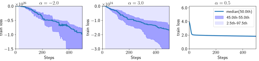
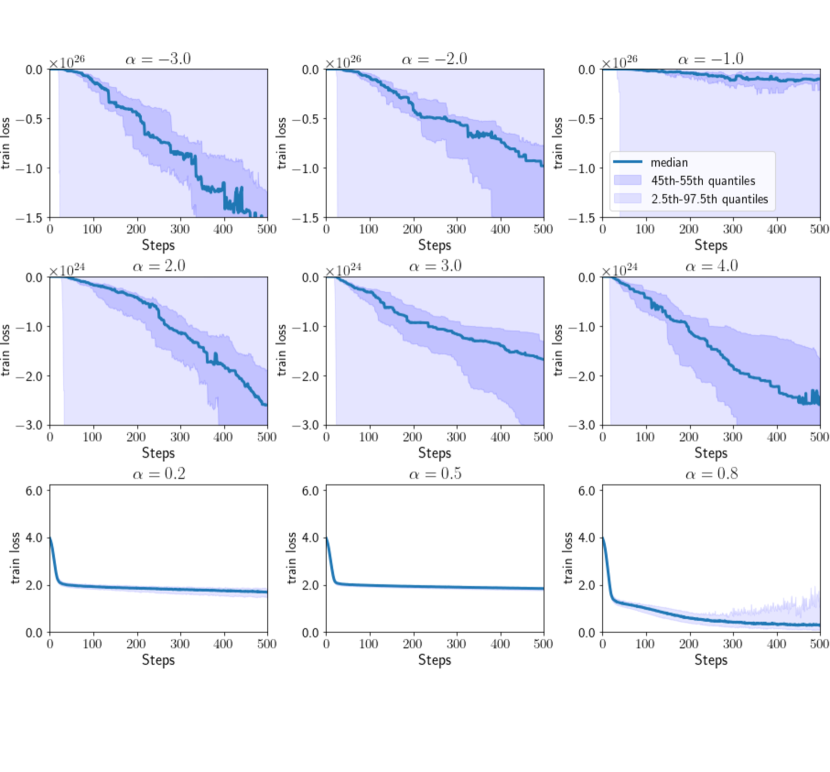
We empirically confirmed the stability of optimization using α\alpha-Div, as discussed in Section 5.1. This includes addressing the potential divergence of training losses for α>1\alpha>1 and α<0\alpha<0, and observing the stability of optimization when α\alpha is within (0,1)(0,1). Subsequently, we conducted experiments using synthetic datasets to examine the behavior of training losses during optimization across different values of α\alpha at each learning step.

Experimental Setup. First, we generated 100 training datasets from two 5-dimensional normal distributions, P=𝒩(μp,I5)P=\mathcal{N}(\mu_{p},I_{5}) and Q=𝒩(μq,Σq)Q=\mathcal{N}(\mu_{q},\Sigma_{q}), where μp=μq=(0,0,,0)\mu_{p}=\mu_{q}=(0,0,\ldots,0), and I5I_{5} denotes the 55-dimensional identity matrix. The covariance matrix Σq=(σij)i=15\Sigma_{q}=(\sigma_{ij})_{i=1}^{5} is defined as σii=1\sigma_{ii}=1, and σij=0.8\sigma_{ij}=0.8 for iji\neq j. Subsequently, we trained neural networks using the synthetic datasets by optimizing α\alpha-Div for α=3.0,2.0,1.0,0.2,0.5,0.8,2.0,3.0\alpha=-3.0,\allowbreak-2.0,\allowbreak-1.0,\allowbreak 0.2,\allowbreak 0.5,\allowbreak 0.8,\allowbreak 2.0,\allowbreak 3.0, and 4.04.0, while measuring training losses at each learning step. For each value of α\alpha, 100 trials were performed. Finally, we reported the median of the training losses at each learning step, along with the ranges between the 45th and 55th percentiles and between the 2.5th and 97.5th percentiles.

Results. Figure 2 presents the training losses of α\alpha-Div across the learning steps for α=2.0,3.0\alpha=-2.0,\allowbreak 3.0, and 0.50.5. Results for other values of α\alpha are provided in Section D.1 in the Appendix. The figures on the left (α=2.0\alpha=-2.0) and in the center (α=3.0\alpha=3.0) show that the training losses diverged to negative infinity when α<0\alpha<0 or α>1\alpha>1. In contrast, the figure on the right (α=0.5\alpha=0.5) demonstrates that the training losses successfully converged. These results highlight the stability of α\alpha-Div’s optimization when α\alpha is within the interval (0,1)(0,1), as discussed in Section 5.1.

6.2 Experiments on the Improvement of Optimization Efficiency by Removing Gradient Bias

Refer to caption

Figure 1: Results from Section 6.1. The left (α=2.0\alpha=-2.0), center (α=3.0\alpha=3.0), and right (α=0.5\alpha=0.5) graphs show training losses (yy-axis) over learning steps (xx-axis) during optimization using α\alpha-Div with different α\alpha values. Solid blue lines represent median training losses, dark blue shaded areas show the 45th to 55th percentiles, and light blue shaded areas represent the 2.5th to 97.5th percentiles.

Refer to caption

Refer to caption

Figure 2: Results from Section 6.2. The top row shows training losses, and the bottom row shows estimated density ratios (DR) during optimization. The left column uses the standard α\alpha-divergence loss function (biased gradients), the center column uses α\alpha-Div (unbiased gradients), and the right column uses nnBD-LSIF (unbiased gradients). The xx-axis represents learning steps. Solid blue lines indicate median values, dark blue shaded areas show the 45th to 55th percentiles, and light blue shaded areas represent the 2.5th to 97.5th percentiles.

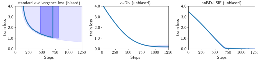
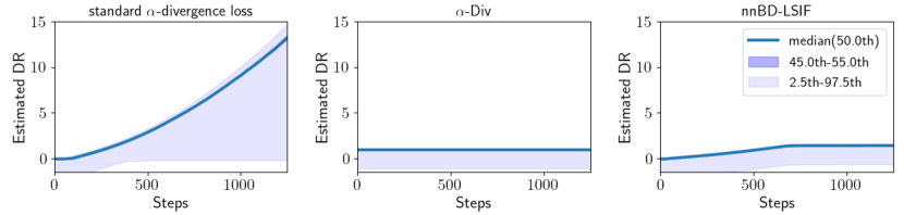
Unbiased gradients of loss functions are expected to optimize neural network parameters more effectively than biased gradients, since they update the parameters in ideal directions at each iteration. We empirically compared the efficiency of minimizing training losses between the proposed loss function and the standard α\alpha-divergence loss function derived from Equation (12), which highlighted the effectiveness of the unbiased gradients of the proposed loss function. Additionally, we observed that the estimated density ratios using the standard α\alpha-divergence loss function diverged to large positive values, suggesting that the gradients of the standard α\alpha-divergence loss function vanished. In contrast, α\alpha-Div exhibited stable estimation. This finding aligns with the discussion in Section 5.3.

Experimental Setup. We first generated 100 training datasets from two normal distributions, P=𝒩(μp,I5)P=\mathcal{N}(\mu_{p},I_{5}) and Q=𝒩(μq,I5)Q=\mathcal{N}(\mu_{q},I_{5}), where I5I_{5} denotes the 5-dimensional identity matrix. The means were set as μp=(5/2,0,0,0,0)\mu_{p}=(-5/2,0,0,0,0) and μq=(5/2,0,0,0,0)\mu_{q}=(5/2,0,0,0,0). We then trained neural networks using three different loss functions: the standard α\alpha-divergence loss function defined in Equation (12), α\alpha-Div, and deep direct DRE (D3RE) [14]. Training losses were measured at each learning step. D3RE addresses train-loss hacking issues associated with Bregman divergence loss functions, as described in Section 3.4, by mitigating the lower-unboundedness of loss functions. Specifically, for D3RE, we employed the neural network-based Bregman divergence Least Squares Importance Fitting (nnBD-LSIF) loss function, which ensures unbiased gradients and stable optimization. The hyperparameter for nnBD-LSIF was set to C=2C=2. For both the standard α\alpha-divergence loss and α\alpha-Div, we used α=0.5\alpha=0.5. Finally, we reported the median training losses at each learning step, along with ranges between the 45th and 55th percentiles and between the 2.5th and 97.5th percentiles.

Results.

The top row in Figure 2 illustrates the training losses at each learning step for each loss function. The center and right panels show that α\alpha-Div and nnBD-LSIF are more effective at minimizing training losses compared to the standard α\alpha-divergence loss function. These findings indicate that the unbiased gradient of α\alpha-Div, like nnBD-LSIF, leads to more efficient neural network optimization than the biased gradient of the standard α\alpha-divergence loss function. These results highlight the ineffectiveness in optimization of the standard α\alpha-divergence loss function inherent in its biased gradients and α\alpha-Div successfully mitigates this issue.

Additionally, the training losses for the standard α\alpha-divergence loss function diverged to positive infinity after 400 steps (the top panel in the left column), and the estimated density ratio diverged during optimization (the bottom panel in the left column). As shown in Table 4, the divergence of both the standard α\alpha-divergence loss function and the estimated density ratio when 0<α<10<\alpha<1, that is α-standard(ϕθ)\mathcal{L}_{\alpha\text{-standard}}(\phi_{\theta})\rightarrow\infty and ϕθ\phi_{\theta}\rightarrow\infty with 0<α<10<\alpha<1, imply that E[θα-standard(ϕθ)]𝟎E\big{[}\nabla_{\theta}\mathcal{L}_{\alpha\text{-standard}}(\phi_{\theta})\big{]}\rightarrow\mathbf{0}. Consequently, these results demonstrate that the vanishing gradient issue in the standard α\alpha-divergence loss function occurs when the estimated density ratio ϕθ\phi_{\theta} becomes very large when 0<α<10<\alpha<1. In contrast, α\alpha-Div avoids this instability by maintaining stable gradients, which aligns with the discussion in Section 5.3.

6.3 Experiments on the Estimation Accuracy Using High KL-Divergence Data
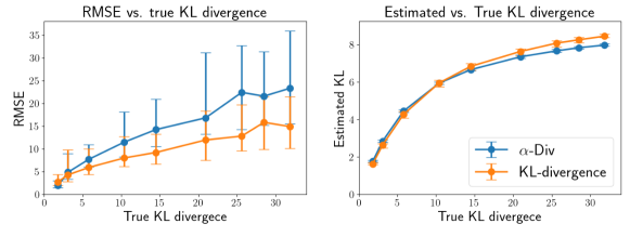
Refer to caption

Figure 3: Results of Section 6.3. The xx-axis represents the ground truth KL-divergence of the data. The yy-axes of the left and right graphs represent the RMSE and estimated KL-divergence, respectively. The plot shows the median yy-axis values for the ground truth KL-divergence. Vertical lines indicate the interquartile range (25th to 75th percentiles) of the yy-axis values.

In Section 3.5, we examined the α\alpha-divergence loss function, hypothesizing that its boundedness could address sample size issues in high KL-divergence data. Theorem 5.2, based on this boundedness, suggests that α\alpha-Div can be minimized regardless of the true KL-divergence, indicating its potential for effective DRE with high KL-divergence data. To validate this hypothesis, we assessed DRE and KL-divergence estimation accuracy using both α\alpha-Div and a KL-divergence loss function.

However, we observed that the RMSE of DRE using α\alpha-Div increased significantly with higher KL-divergence, similar to the KL-divergence loss function.

Additionally, both methods yielded nearly identical KL-divergence estimations. These findings suggest that the accuracy of DRE and KL-divergence estimation is primarily influenced by the true amount of KL-divergence in the data rather than the α\alpha-divergence.

Experimental Setup. We generated 100 training and 100 test datasets, each containing 10,000 samples. The datasets were drawn from two normal distributions, P=𝒩(μp,σ2I3)P=\mathcal{N}(\mu_{p},\sigma^{2}\cdot I_{3}) and Q=𝒩(μq,42I3)Q=\mathcal{N}(\mu_{q},4^{2}\cdot I_{3}), where μp=(3/2,3/2,3/2)\mu_{p}=(-3/2,-3/2,-3/2) and μq=(3/2,3/2,3/2)\mu_{q}=(3/2,3/2,3/2), with I3I_{3} denoting the 3-dimensional identity matrix. The values of σ\sigma were set to 1.0, 1.1, 1.2, 1.4, 1.6, 2.0, 2.5, and 3.0. Correspondingly, the ground truth KL-divergence values of the datasets were 31.8, 25.6, 21.0, 14.5, 10.4, 5.8, 3.1, and 1.8 nats111A ’nat’ is a unit of information measured using the natural logarithm (base ee), reflecting the increasing σ2\sigma^{2} values. The true density ratios of the test datasets are known for this experimental setup. We trained neural networks on the training datasets by optimizing both α\alpha-Div with α=0.5\alpha=0.5 and the KL-divergence loss function. After training, we measured the root mean squared error (RMSE) of the estimated density ratios using the test datasets. Additionally, we estimated the KL-divergence of the test datasets based on the estimated density ratios using a plug-in estimator. Finally, we reported the median RMSE of the DRE and the estimated KL-divergence, along with the interquartile range (25th to 75th percentiles), for both the KL-divergence loss function and α\alpha-Div.

Results. Figure 3 shows the experimental results. The xx-axis represents the true KL-divergence values of the test datasets, while the y-axes of the graphs display the RMSE (left) and estimated KL-divergence (right) for the test datasets. We empirically observed that the RMSE for DRE using α\alpha-Div increased significantly as the KL-divergence of the datasets increased. A similar trend was observed for the KL-divergence loss function. Additionally, the KL-divergence estimation results were nearly identical between both methods. These findings indicate that the accuracy of DRE and KL-divergence estimation is primarily determined by the magnitude of KL-divergence in the data and is less influenced by α\alpha-divergence. Therefore, we conclude that the approach discussed in Section 5.4 offers no advantage over the KL-divergence loss function in terms of the RMSE for DRE with high KL-divergence data. However, we believe that these empirical findings contribute to a deeper understanding of the accuracy of downstream tasks in DRE using ff-divergence loss functions.

7 Conclusion

This study introduced a novel loss function for DRE, α\alpha-Div, which is both concise and provides stable, efficient optimization. We offered technical justifications and demonstrated its effectiveness through numerical experiments. The empirical results confirmed the efficiency of the proposed loss function. However, experiments with high KL-divergence data revealed that the α\alpha-divergence loss function did not offer a significant advantage over the KL-divergence loss function in terms of RMSE for DRE. These findings contribute to a deeper understanding of the accuracy of downstream tasks in DRE when using ff-divergence loss functions.

References

  • Amari and Nagaoka [2000] Shun-ichi Amari and Hiroshi Nagaoka. Methods of information geometry, volume 191. American Mathematical Soc., 2000.
  • Arjovsky and Bottou [2017] Martin Arjovsky and Léon Bottou. Towards principled methods for training generative adversarial networks. arXiv preprint arXiv:1701.04862, 2017.
  • Belghazi et al. [2018] Mohamed Ishmael Belghazi, Aristide Baratin, Sai Rajeshwar, Sherjil Ozair, Yoshua Bengio, Aaron Courville, and Devon Hjelm. Mutual information neural estimation. In International conference on machine learning, pages 531–540. PMLR, 2018.
  • Bingham and Mannila [2001] Ella Bingham and Heikki Mannila. Random projection in dimensionality reduction: applications to image and text data. In Proceedings of the seventh ACM SIGKDD international conference on Knowledge discovery and data mining, pages 245–250, 2001.
  • Birrell et al. [2021] Jeremiah Birrell, Paul Dupuis, Markos A Katsoulakis, Luc Rey-Bellet, and Jie Wang. Variational representations and neural network estimation of rényi divergences. SIAM Journal on Mathematics of Data Science, 3(4):1093–1116, 2021.
  • Blitzer et al. [2007] John Blitzer, Mark Dredze, and Fernando Pereira. Biographies, bollywood, boom-boxes and blenders: Domain adaptation for sentiment classification. In Proceedings of the 45th annual meeting of the association of computational linguistics, pages 440–447, 2007.
  • Cai et al. [2020] Likun Cai, Yanjie Chen, Ning Cai, Wei Cheng, and Hao Wang. Utilizing amari-alpha divergence to stabilize the training of generative adversarial networks. Entropy, 22(4):410, 2020.
  • Choi et al. [2022] Kristy Choi, Chenlin Meng, Yang Song, and Stefano Ermon. Density ratio estimation via infinitesimal classification. In International Conference on Artificial Intelligence and Statistics, pages 2552–2573. PMLR, 2022.
  • Goodfellow et al. [2014] Ian Goodfellow, Jean Pouget-Abadie, Mehdi Mirza, Bing Xu, David Warde-Farley, Sherjil Ozair, Aaron Courville, and Yoshua Bengio. Generative adversarial nets. Advances in neural information processing systems, 27, 2014.
  • Gutmann and Hyvärinen [2010] Michael Gutmann and Aapo Hyvärinen. Noise-contrastive estimation: A new estimation principle for unnormalized statistical models. In Proceedings of the thirteenth international conference on artificial intelligence and statistics, pages 297–304. JMLR Workshop and Conference Proceedings, 2010.
  • Hjelm et al. [2018] R Devon Hjelm, Alex Fedorov, Samuel Lavoie-Marchildon, Karan Grewal, Phil Bachman, Adam Trischler, and Yoshua Bengio. Learning deep representations by mutual information estimation and maximization. arXiv preprint arXiv:1808.06670, 2018.
  • Huang et al. [2006] Jiayuan Huang, Arthur Gretton, Karsten Borgwardt, Bernhard Schölkopf, and Alex Smola. Correcting sample selection bias by unlabeled data. Advances in neural information processing systems, 19, 2006.
  • Kanamori et al. [2009] Takafumi Kanamori, Shohei Hido, and Masashi Sugiyama. A least-squares approach to direct importance estimation. The Journal of Machine Learning Research, 10:1391–1445, 2009.
  • Kato and Teshima [2021] Masahiro Kato and Takeshi Teshima. Non-negative bregman divergence minimization for deep direct density ratio estimation. In International Conference on Machine Learning, pages 5320–5333. PMLR, 2021.
  • Kato et al. [2019] Masahiro Kato, Takeshi Teshima, and Junya Honda. Learning from positive and unlabeled data with a selection bias. In International conference on learning representations, 2019.
  • Ke et al. [2017] Guolin Ke, Qi Meng, Thomas Finley, Taifeng Wang, Wei Chen, Weidong Ma, Qiwei Ye, and Tie-Yan Liu. Lightgbm: A highly efficient gradient boosting decision tree. Advances in neural information processing systems, 30, 2017.
  • Kingma [2014] Diederik P Kingma. Adam: A method for stochastic optimization. arXiv preprint arXiv:1412.6980, 2014.
  • Kwon and Baek [2024] Euijoon Kwon and Yongjoo Baek. α\alpha-divergence improves the entropy production estimation via machine learning. Physical Review E, 109(1):014143, 2024.
  • McAllester and Stratos [2020] David McAllester and Karl Stratos. Formal limitations on the measurement of mutual information. In International Conference on Artificial Intelligence and Statistics, pages 875–884. PMLR, 2020.
  • Menon and Ong [2016] Aditya Menon and Cheng Soon Ong. Linking losses for density ratio and class-probability estimation. In International Conference on Machine Learning, pages 304–313. PMLR, 2016.
  • Nguyen et al. [2007] XuanLong Nguyen, Martin J Wainwright, and Michael Jordan. Estimating divergence functionals and the likelihood ratio by penalized convex risk minimization. Advances in neural information processing systems, 20, 2007.
  • Nguyen et al. [2010] XuanLong Nguyen, Martin J Wainwright, and Michael I Jordan. Estimating divergence functionals and the likelihood ratio by convex risk minimization. IEEE Transactions on Information Theory, 56(11):5847–5861, 2010.
  • Nowozin et al. [2016] Sebastian Nowozin, Botond Cseke, and Ryota Tomioka. f-gan: Training generative neural samplers using variational divergence minimization. Advances in neural information processing systems, 29, 2016.
  • Paszke et al. [2017] Adam Paszke, Sam Gross, Soumith Chintala, Gregory Chanan, Edward Yang, Zachary DeVito, Zeming Lin, Alban Desmaison, Luca Antiga, and Adam Lerer. Automatic differentiation in pytorch. 2017.
  • Pedregosa et al. [2011] Fabian Pedregosa, Gaël Varoquaux, Alexandre Gramfort, Vincent Michel, Bertrand Thirion, Olivier Grisel, Mathieu Blondel, Peter Prettenhofer, Ron Weiss, Vincent Dubourg, et al. Scikit-learn: Machine learning in python. the Journal of machine Learning research, 12:2825–2830, 2011.
  • Poole et al. [2019] Ben Poole, Sherjil Ozair, Aaron Van Den Oord, Alex Alemi, and George Tucker. On variational bounds of mutual information. In International Conference on Machine Learning, pages 5171–5180. PMLR, 2019.
  • Ragab et al. [2023] Mohamed Ragab, Emadeldeen Eldele, Wee Ling Tan, Chuan-Sheng Foo, Zhenghua Chen, Min Wu, Chee-Keong Kwoh, and Xiaoli Li. Adatime: A benchmarking suite for domain adaptation on time series data. ACM Transactions on Knowledge Discovery from Data, 17(8):1–18, 2023.
  • Rhodes et al. [2020] Benjamin Rhodes, Kai Xu, and Michael U Gutmann. Telescoping density-ratio estimation. Advances in neural information processing systems, 33:4905–4916, 2020.
  • Shimodaira [2000] Hidetoshi Shimodaira. Improving predictive inference under covariate shift by weighting the log-likelihood function. Journal of statistical planning and inference, 90(2):227–244, 2000.
  • Shiryaev [1995] Albert Nikolaevich Shiryaev. Probability, 1995.
  • Song and Ermon [2019] Jiaming Song and Stefano Ermon. Understanding the limitations of variational mutual information estimators. arXiv preprint arXiv:1910.06222, 2019.
  • Sugiyama et al. [2007a] Masashi Sugiyama, Matthias Krauledat, and Klaus-Robert Müller. Covariate shift adaptation by importance weighted cross validation. Journal of Machine Learning Research, 8(5), 2007a.
  • Sugiyama et al. [2007b] Masashi Sugiyama, Shinichi Nakajima, Hisashi Kashima, Paul Buenau, and Motoaki Kawanabe. Direct importance estimation with model selection and its application to covariate shift adaptation. Advances in neural information processing systems, 20, 2007b.
  • Sugiyama et al. [2012] Masashi Sugiyama, Taiji Suzuki, and Takafumi Kanamori. Density-ratio matching under the bregman divergence: a unified framework of density-ratio estimation. Annals of the Institute of Statistical Mathematics, 64:1009–1044, 2012.
  • Uehara et al. [2016] Masatoshi Uehara, Issei Sato, Masahiro Suzuki, Kotaro Nakayama, and Yutaka Matsuo. Generative adversarial nets from a density ratio estimation perspective. arXiv preprint arXiv:1610.02920, 2016.

Appendix A Organization of the Supplementary Document

The organization of this supplementary document is as follows: Section B reviews prior work in DRE using ff-divergence optimization. Section C presents the theorems and proofs cited in this study. Section D provides details of the numerical experiments conducted. Finally, Section E presents additional experimental results.

Appendix B Related Work

Nguyen et al. [22] proposed DRE using variational representations of ff-divergences. Sugiyama et al. [34] introduced density-ratio matching under the Bregman divergence, a general framework that unifies various methods for DRE. As noted by Sugiyama et al. [34], density-ratio matching under the Bregman divergence is equivalent to DRE using variational representations of ff-divergences. Kato and Teshima [14] proposed a correction method for Bregman divergence loss functions s, in which the loss functions diverge to negative infinity, as discussed in Section 3.2. For estimation in scenarios with high KL-divergence data, Rhodes et al. [28] proposed a method that divides the high KL-divergence estimation into multiple smaller divergence estimations. Choi et al. [8] further developed a continuous decomposition approach by introducing an auxiliary variable for transforming the data distribution. DRE using variational representations of ff-divergences has also been studied from the perspective of classification-based modeling. Menon and Ong [20] demonstrated that DRE via ff-divergence optimization can be represented as a binary classification problem. Kato et al. [15] proposed using the risk functions in PU learning for DRE.

Lastly, we review prior studies on DRE focusing on α\alpha-divergence loss functions. Birrell et al. [5] derived an α\alpha-divergence loss function from Rényi’s α\alpha-divergence, while Cai et al. [7] employed a standard variational representation of Amari’s α\alpha-divergence with α<0\alpha<0 or α>1\alpha>1. Kwon and Baek [18] presented essentially the same α\alpha-divergence loss function proposed in this study, utilizing the Gibbs density expression to measure entropy in thermodynamics. In contrast, we propose the loss function to address the biased gradient problem.

Appendix C Proofs

In this section, we present the theorems and the proofs referenced in this study. First, we define α\alpha-Div within a probabilistic theoretical framework. Following that, we provide the theorems and the proofs cited throughout the study.

Capital, small and bold letters.

Random variables are denoted by capital letters. For example, XX. Small letters are used for values of the random variables corresponding to the capital letters; aa denotes a value of the random variable XX. Bold letters 𝐗\mathbf{X} and 𝐱\mathbf{x} represent sets of random variables and their values.

C.1 Definition of α\alpha-Div

Definition C.1 (α\alpha-Divergence loss).

Let 𝐗P1,𝐗P2,,𝐗PR\mathbf{X}^{1}_{P},\mathbf{X}^{2}_{P},\ldots,\mathbf{X}^{R}_{P} denote RR i.i.d. random variables drawn from PP, and let 𝐗Q1,𝐗Q2,,𝐗QS\mathbf{X}^{1}_{Q},\mathbf{X}^{2}_{Q},\ldots,\mathbf{X}^{S}_{Q} denote SS i.i.d. random variables drawn from QQ. Then, the α\alpha-Divergence loss α-Div(R,S)(;α)\mathcal{L}_{\alpha\text{-Div}}^{(R,S)}(\cdot\,;\,\alpha) is defined as follows:

α-Div(R,S)(T;α)=1α1Si=1SeαT(𝐗Qi)+11α1Ri=1Re(α1)T(𝐗Pi),\mathcal{L}_{\alpha\text{-Div}}^{(R,S)}(T\,;\,\alpha)=\frac{1}{\alpha}\cdot\frac{1}{S}\cdot\sum_{i=1}^{S}e^{\alpha\cdot T(\mathbf{X}^{i}_{Q})}+\frac{1}{1-\alpha}\cdot\frac{1}{R}\cdot\sum_{i=1}^{R}e^{(\alpha-1)\cdot T(\mathbf{X}^{i}_{P})}, (17)

where TT is a measurable function over Ω\Omega such that T:ΩT:\Omega\rightarrow\mathbb{R}.

C.2 Proofs for Section 4

In this section, we provide the theorems and the proofs referenced in Section 4.

Theorem C.2.

A variational representation of α\alpha-divergence is given as

D(Q||P;α)\displaystyle D(Q||P\,;\,\alpha) =supϕ0{1α(1α)1αEQ[ϕα]11αEP[ϕ1α]},\displaystyle=\sup_{\phi\geq 0}\left\{\frac{1}{\alpha\cdot(1-\alpha)}-\frac{1}{\alpha}\cdot E_{Q}\left[\phi^{-\alpha}\right]-\frac{1}{1-\alpha}\cdot E_{P}\left[\phi^{1-\alpha}\right]\right\}, (18)

where the supremum is taken over all measurable functions with EP[ϕ1α]<E_{P}[\phi^{1-\alpha}]<\infty and EQ[ϕα]<E_{Q}[\phi^{-\alpha}]<\infty. The maximum value is achieved at ϕ=dQ/dP\phi=dQ/dP.

Proof of Theorem C.2.

Let fα(t)={t1α(1α)tα}/{α(α1)}f_{\alpha}(t)=\{t^{1-\alpha}-(1-\alpha)\cdot t-\alpha\}/\{\alpha\cdot(\alpha-1)\} for α0,1\alpha\neq 0,1, then

EP[fα(dQdP)]\displaystyle E_{P}\left[f_{\alpha}\left(\frac{dQ}{dP}\right)\right] =EP[1α(1α)(dQdP)1α+1α(dQdP)+11α]\displaystyle=E_{P}\left[\frac{1}{\alpha\cdot(1-\alpha)}\cdot\left(\frac{dQ}{dP}\right)^{1-\alpha}+\frac{1}{\alpha}\cdot\left(\frac{dQ}{dP}\right)+\frac{1}{1-\alpha}\right]
=1α(1α)EP[(dQdP)1α]+1α+11α\displaystyle=\frac{1}{\alpha\cdot(1-\alpha)}\cdot E_{P}\left[\left(\frac{dQ}{dP}\right)^{1-\alpha}\right]+\frac{1}{\alpha}+\frac{1}{1-\alpha}
=D(Q||P;α).\displaystyle=D(Q||P\,;\,\alpha). (19)

Note that, the Legendre transform of gα(x)=x1α/(1α)g_{\alpha}(x)=x^{1-\alpha}/(1-\alpha) is obtained as

gα(x)=αα1x11α,g_{\alpha}^{*}(x)=\frac{\alpha}{\alpha-1}\cdot x^{1-\frac{1}{\alpha}}, (20)

and for the Legendre transforms of functions, it holds that

{Ch(x)}=Ch(xC)and{h(x)+Cx+D}=h(xC)D.\{C\cdot h(x)\}^{*}=C\cdot h^{*}\left(\frac{x}{C}\right)\quad\text{and}\quad\{h(x)+C\cdot x+D\}^{*}=h^{*}(x-C)-D. (21)

Here, AA^{*} denotes the Legendre transform of AA.

From Equations (20) and (21), we have

fα(t)\displaystyle f_{\alpha}^{*}(t) ={1(α)gα(t)+1αt+11α}\displaystyle=\left\{\frac{1}{(-\alpha)}\cdot g_{\alpha}(t)+\frac{1}{\alpha}\cdot t+\frac{1}{1-\alpha}\right\}^{*}
=1(α)gα(α{t1α})11α\displaystyle=\frac{1}{(-\alpha)}\cdot g_{\alpha}^{*}\left(-\alpha\cdot\left\{t-\frac{1}{\alpha}\right\}\right)-\frac{1}{1-\alpha}
=1αgα(1αt)+1α1\displaystyle=-\frac{1}{\alpha}\cdot g_{\alpha}^{*}\left(1-\alpha t\right)+\frac{1}{\alpha-1}
=1α{αα1(1αt)11α}+1α1\displaystyle=-\frac{1}{\alpha}\cdot\left\{\frac{\alpha}{\alpha-1}\cdot\left(1-\alpha t\right)^{1-\frac{1}{\alpha}}\right\}+\frac{1}{\alpha-1}
=11α(1αt)11α+1α1.\displaystyle=\frac{1}{1-\alpha}\cdot\left(1-\alpha t\right)^{1-\frac{1}{\alpha}}+\frac{1}{\alpha-1}. (22)

By differentiating fα(t)f_{\alpha}(t), we obtain

fα(t)=1αtα+1α.f_{\alpha}^{\prime}(t)=-\frac{1}{\alpha}\cdot t^{-\alpha}+\frac{1}{\alpha}. (23)

Thus,

EQ[fα(ϕ)]=EQ[1αϕα+1α].\displaystyle E_{Q}\big{[}f_{\alpha}^{\prime}(\phi)\big{]}=E_{Q}\left[-\frac{1}{\alpha}\cdot\phi^{-\alpha}+\frac{1}{\alpha}\right]. (24)

From (22) and (23), we have

EP[fα(fα(ϕ))]\displaystyle E_{P}\big{[}f_{\alpha}^{*}(f_{\alpha}^{\prime}(\phi))\big{]} =EP[11α{1α(1αϕα+1α)}11α+1α1]\displaystyle=E_{P}\left[\frac{1}{1-\alpha}\cdot\left\{1-\alpha\cdot\left(-\frac{1}{\alpha}\cdot\phi^{-\alpha}+\frac{1}{\alpha}\right)\right\}^{1-\frac{1}{\alpha}}+\frac{1}{\alpha-1}\right]
=EP[11αϕ1α+1α1].\displaystyle=E_{P}\left[\frac{1}{1-\alpha}\cdot\phi^{1-\alpha}+\frac{1}{\alpha-1}\right]. (25)

In addition, from Equations (24) and (25), we observe that EP[ϕ1α]<E_{P}\big{[}\phi^{1-\alpha}\big{]}<\infty is equivalent to EP[|fα(fα(ϕ))|]<E_{P}\big{[}\,\big{|}f_{\alpha}^{*}(f_{\alpha}^{\prime}(\phi))\big{|}\,\big{]}<\infty. Similarly, EQ[ϕα]<E_{Q}\big{[}\phi^{-\alpha}\big{]}<\infty is equivalent to EQ[|fα(ϕ)|]<E_{Q}\big{[}\,\big{|}f_{\alpha}^{\prime}(\phi)\big{|}\,\big{]}<\infty.

Finally, by substituting Equations (24) and (25) into Equation (1), we get

D(Q||P;α)\displaystyle D(Q||P\,;\,\alpha) =supϕ0{EQ[fα(ϕ)]EP[fα(fα(ϕ))]}\displaystyle=\sup_{\phi\geq 0}\Big{\{}E_{Q}\big{[}f_{\alpha}^{\prime}(\phi)\big{]}-E_{P}\big{[}f_{\alpha}^{*}(f_{\alpha}^{\prime}(\phi))\big{]}\Big{\}}
=supϕ0{EQ[1αϕα+1α]EP[11αϕ1α+1α1]}\displaystyle=\sup_{\phi\geq 0}\left\{E_{Q}\left[-\frac{1}{\alpha}\cdot\phi^{-\alpha}+\frac{1}{\alpha}\right]-E_{P}\left[\frac{1}{1-\alpha}\cdot\phi^{1-\alpha}+\frac{1}{\alpha-1}\right]\right\}
=supϕ0{1α(1α)1αEQ[ϕα]11αEP[ϕ1α]}.\displaystyle=\sup_{\phi\geq 0}\left\{\frac{1}{\alpha\cdot(1-\alpha)}-\frac{1}{\alpha}\cdot E_{Q}\left[\phi^{-\alpha}\right]-\frac{1}{1-\alpha}\cdot E_{P}\left[\phi^{1-\alpha}\right]\right\}.

This completes the proof. ∎

Theorem C.3 (Theorem 4.2 in Section 4 restated).

The α\alpha-divergence is represented as

D(Q||P;α)=supT:Ω{1α(1α)1αEQ[eαT]11αEP[e(α1)T]},D(Q||P\,;\,\alpha)=\sup_{T:\Omega\rightarrow\mathbb{R}}\left\{\frac{1}{\alpha\cdot(1-\alpha)}-\frac{1}{\alpha}\cdot E_{Q}\left[e^{\alpha\cdot T}\right]-\frac{1}{1-\alpha}\cdot E_{P}\left[e^{(\alpha-1)\cdot T}\right]\right\}, (26)

where the supremum is taken over all measurable functions T:ΩT:\Omega\rightarrow\mathbb{R} with EP[e(α1)T]<E_{P}[e^{(\alpha-1)\cdot T}]<\infty and EQ[eαT]<E_{Q}[e^{\alpha\cdot T}]<\infty. The equality holds for TT^{*} satisfying

dQdP=eT.\frac{dQ}{dP}=e^{-T^{*}}. (27)
proof of Theorem 4.2.

Substituting eTe^{-T} into ϕ\phi in Equation (18), we have

D(Q||P;α)\displaystyle D(Q||P\,;\,\alpha) =supϕ0{1α(1α)1αEQ[ϕα]11αEP[ϕ1α]}\displaystyle=\sup_{\phi\geq 0}\left\{\frac{1}{\alpha\cdot(1-\alpha)}-\frac{1}{\alpha}\cdot E_{Q}\left[\phi^{-\alpha}\right]-\frac{1}{1-\alpha}\cdot E_{P}\left[\phi^{1-\alpha}\right]\right\}
=supT:Ω{1α(1α)1αEQ[{eT}α]11αEP[{eT}1α]}\displaystyle=\sup_{T:\Omega\rightarrow\mathbb{R}}\left\{\frac{1}{\alpha\cdot(1-\alpha)}-\frac{1}{\alpha}\cdot E_{Q}\left[\left\{e^{-T}\right\}^{-\alpha}\right]-\frac{1}{1-\alpha}\cdot E_{P}\left[\left\{e^{-T}\right\}^{1-\alpha}\right]\right\}
=supT:Ω{1α(1α)1αEQ[eαT]11αEP[e(α1)T]}.\displaystyle=\sup_{T:\Omega\rightarrow\mathbb{R}}\left\{\frac{1}{\alpha\cdot(1-\alpha)}-\frac{1}{\alpha}\cdot E_{Q}\left[e^{\alpha\cdot T}\right]-\frac{1}{1-\alpha}\cdot E_{P}\left[e^{(\alpha-1)\cdot T}\right]\right\}. (28)

Finally, from Theorem 4.1, the equality for Equation (28) holds if and only if

dQdP=eT.\frac{dQ}{dP}=e^{-T^{*}}. (29)

This completes the proof. ∎

Lemma C.4.

For a measurable function T:ΩT:\Omega\rightarrow\mathbb{R} with EP[e(α1)T]<E_{P}[e^{(\alpha-1)\cdot T}]<\infty and EQ[eαT]<E_{Q}[e^{\alpha\cdot T}]<\infty, let

l~α-Div(T(𝐱);α)\displaystyle\widetilde{l}_{\alpha\text{-Div}}\left(T(\mathbf{x})\,;\,\alpha\right) =1αeαT(𝐱)dQdμ(𝐱)+11αe(α1)T(𝐱)dPdμ(𝐱).\displaystyle=\frac{1}{\alpha}\cdot e^{\alpha\cdot T(\mathbf{x})}\cdot\frac{dQ}{d\mu}(\mathbf{x})+\frac{1}{1-\alpha}\cdot e^{(\alpha-1)\cdot T(\mathbf{x})}\cdot\frac{dP}{d\mu}(\mathbf{x}). (30)

Then the optimal function TT^{*} for infT:Ωl~α-Div(T;α)\inf_{T:\Omega\rightarrow\mathbb{R}}\widetilde{l}_{\alpha\text{-Div}}\left(T\,;\,\alpha\right) is obtained as T=logdQ/dPT^{*}=-\log dQ/dP, μ\mu-almost everywhere.

proof of Lemma C.4.

First, note that it follows from Jensen’s inequality that

log(pX+qY)plog(X)+qlog(Y),\log(p\cdot X+q\cdot Y)\geq p\cdot\log(X)+q\cdot\log(Y), (31)

for X,Y>0X,Y>0 and p,q>0p,q>0 with p+q=1p+q=1, and equality holds when X=YX=Y.

Substitute X=eαT(𝐱)dQdμ(𝐱)X=e^{\alpha\cdot T(\mathbf{x})}\cdot\frac{dQ}{d\mu}(\mathbf{x}), Y=e(α1)T(𝐱)dPdμ(𝐱)Y=e^{(\alpha-1)\cdot T(\mathbf{x})}\cdot\frac{dP}{d\mu}(\mathbf{x}), p=1αp=1-\alpha, and q=αq=\alpha into Equation (31), we obtain

log(pX+qY)=log(1α(1α)l~α-Div(T;α)),\log(p\cdot X+q\cdot Y)=\log\left(\frac{1}{\alpha\cdot(1-\alpha)}\cdot\widetilde{l}_{\alpha\text{-Div}}(T\,;\,\alpha)\right),

and log(1α(1α)l~α-Div(T;α))\log\left(\frac{1}{\alpha\cdot(1-\alpha)}\cdot\widetilde{l}_{\alpha\text{-Div}}(T\,;\,\alpha)\right) is minimized when eαT(𝐱)dQdμ(𝐱)=e(α1)T(𝐱)dPdμ(𝐱)e^{\alpha\cdot T(\mathbf{x})}\cdot\frac{dQ}{d\mu}(\mathbf{x})=e^{(\alpha-1)\cdot T(\mathbf{x})}\cdot\frac{dP}{d\mu}(\mathbf{x}), μ\mu-almost everywhere. Therefore, infT:Ωl~α-Div(T;α)\inf_{T:\Omega\rightarrow\mathbb{R}}\widetilde{l}_{\alpha\text{-Div}}(T\,;\,\alpha) is achieved at eT(𝐱)=dQdP(𝐱)e^{-T^{*}(\mathbf{x})}=\frac{dQ}{dP}(\mathbf{x}), μ\mu-almost everywhere. Thus, we obtain T(𝐱)=logdQdP(𝐱)T^{*}(\mathbf{x})=-\log\frac{dQ}{dP}(\mathbf{x}), μ\mu-almost everywhere.

This completes the proof. ∎

Lemma C.5.

For a measurable function T:ΩT:\Omega\rightarrow\mathbb{R} with EP[e(α1)T]<E_{P}[e^{(\alpha-1)\cdot T}]<\infty and EQ[eαT]<E_{Q}[e^{\alpha\cdot T}]<\infty, let

\macc@depthΔ\frozen@everymath\macc@group\macc@set@skewchar\macc@nested@a111α-Div(T;α\displaystyle\macc@depth\char 1\relax\frozen@everymath{\macc@group}\macc@set@skewchar\macc@nested@a 111{\mathcal{L}}_{\alpha\text{-Div}}(T\,;\,\alpha =Eμ[l~α-Div(T(𝐱;α))]\displaystyle=E_{\mu}\left[\widetilde{l}_{\alpha\text{-Div}}\left(T(\mathbf{x}\,;\,\alpha)\right)\right] (32)
=1αEQ[eαT(𝐱)]+11αEP[e(α1)T(𝐱)],\displaystyle=\frac{1}{\alpha}\cdot E_{Q}\left[e^{\alpha\cdot T(\mathbf{x})}\right]+\frac{1}{1-\alpha}\cdot E_{P}\left[e^{(\alpha-1)\cdot T(\mathbf{x})}\right], (33)

and let

l~α-Div(α)\displaystyle\widetilde{l}_{\alpha\text{-Div}}^{*}(\alpha) =infT:Ωl~α-Div(T;α),and\displaystyle=\inf_{T:\Omega\rightarrow\mathbb{R}}\widetilde{l}_{\alpha\text{-Div}}(T\,;\,\alpha),\quad\text{and} (34)
\macc@depthΔ\frozen@everymath\macc@group\macc@set@skewchar\macc@nested@a111α-Div(α)\displaystyle\macc@depth\char 1\relax\frozen@everymath{\macc@group}\macc@set@skewchar\macc@nested@a 111{\mathcal{L}}_{\alpha\text{-Div}}^{*}(\alpha) =infT:Ω\macc@depthΔ\frozen@everymath\macc@group\macc@set@skewchar\macc@nested@a111α-Div(T;α),\displaystyle=\inf_{T:\Omega\rightarrow\mathbb{R}}\macc@depth\char 1\relax\frozen@everymath{\macc@group}\macc@set@skewchar\macc@nested@a 111{\mathcal{L}}_{\alpha\text{-Div}}(T\,;\,\alpha), (35)

where the infima of Equations (34) and (35) are considered over measurable functions T:ΩT:\Omega\rightarrow\mathbb{R} with EP[e(α1)T]<E_{P}[e^{(\alpha-1)\cdot T}]<\infty and EQ[eαT]<E_{Q}[e^{\alpha\cdot T}]<\infty.

Then,

Eμ[l~α-Div(α)]=\macc@depthΔ\frozen@everymath\macc@group\macc@set@skewchar\macc@nested@a111α-Div(α).E_{\mu}\left[\widetilde{l}_{\alpha\text{-Div}}^{*}(\alpha)\right]=\macc@depth\char 1\relax\frozen@everymath{\macc@group}\macc@set@skewchar\macc@nested@a 111{\mathcal{L}}_{\alpha\text{-Div}}^{*}(\alpha). (36)

Additionally, the equality in Equations (34) and (35) hold for T(𝐱)=logdQ/dP(𝐱)T^{*}(\mathbf{x})=-\log dQ/dP(\mathbf{x}).

proof of Lemma C.5.

Let T(𝐱)=logdQ/dP(𝐱)T^{*}(\mathbf{x})=-\log dQ/dP(\mathbf{x}).

First, it follows from Lemma C.4 that

l~α-Div(α)=infT:Ωl~α-Div(T;α)=l~α-Div(T;α).\widetilde{l}_{\alpha\text{-Div}}^{*}(\alpha)=\inf_{T:\Omega\rightarrow\mathbb{R}}\widetilde{l}_{\alpha\text{-Div}}(T\,;\,\alpha)=\widetilde{l}_{\alpha\text{-Div}}(T^{*}\,;\,\alpha). (37)

Next, we obtain

Eμ[1α(1α)l~α-Div(α)]\displaystyle E_{\mu}\left[\frac{1}{\alpha\cdot(1-\alpha)}-\widetilde{l}_{\alpha\text{-Div}}^{*}(\alpha)\right] ={1α(1α)l~α-Div(α)}𝑑μ\displaystyle=\int\left\{\frac{1}{\alpha\cdot(1-\alpha)}-\widetilde{l}_{\alpha\text{-Div}}^{*}(\alpha)\right\}d\mu
={1α(1α)infT:Ωl~α-Div(T;α)}𝑑μ\displaystyle=\int\left\{\frac{1}{\alpha\cdot(1-\alpha)}-\inf_{T:\Omega\rightarrow\mathbb{R}}\widetilde{l}_{\alpha\text{-Div}}(T\,;\,\alpha)\right\}d\mu
=supT:Ω{1α(1α)l~α-Div(T;α)}dμ.\displaystyle=\int\sup_{T:\Omega\rightarrow\mathbb{R}}\left\{\frac{1}{\alpha\cdot(1-\alpha)}-\widetilde{l}_{\alpha\text{-Div}}(T\,;\,\alpha)\right\}d\mu. (38)

Let Tk=T+1/kT_{k}=T^{*}+1/k. Note that,

limkl~α-Div(Tk;α)=infT:Ωl~α-Div(T;α)=l~α-Div(α).\lim_{k\rightarrow\infty}\widetilde{l}_{\alpha\text{-Div}}(T_{k}\,;\,\alpha)=\inf_{T:\Omega\rightarrow\mathbb{R}}\widetilde{l}_{\alpha\text{-Div}}(T\,;\,\alpha)=\widetilde{l}_{\alpha\text{-Div}}^{*}(\alpha). (39)

Then, we have

limk{1α(1α)l~α-Div(Tk;α)}\displaystyle\lim_{k\rightarrow\infty}\bigg{\{}\frac{1}{\alpha\cdot(1-\alpha)}-\widetilde{l}_{\alpha\text{-Div}}(T_{k}\,;\,\alpha)\bigg{\}}
=1α(1α)limk{l~α-Div(Tk;α)}\displaystyle=\frac{1}{\alpha\cdot(1-\alpha)}-\lim_{k\rightarrow\infty}\bigg{\{}\widetilde{l}_{\alpha\text{-Div}}(T_{k}\,;\,\alpha)\bigg{\}}
=1α(1α)infT:Ωl~α-Div(T;α)\displaystyle=\frac{1}{\alpha\cdot(1-\alpha)}-\inf_{T:\Omega\rightarrow\mathbb{R}}\widetilde{l}_{\alpha\text{-Div}}(T\,;\,\alpha)
=supT:Ω{1α(1α)l~α-Div(T;α)}.\displaystyle=\sup_{T:\Omega\rightarrow\mathbb{R}}\bigg{\{}\frac{1}{\alpha\cdot(1-\alpha)}-\widetilde{l}_{\alpha\text{-Div}}(T\,;\,\alpha)\bigg{\}}. (40)

From Theorem C.3, we have

limkEμ[1α(1α)l~α-Div(Tk;α)]\displaystyle\lim_{k\rightarrow\infty}E_{\mu}\left[\frac{1}{\alpha\cdot(1-\alpha)}-\widetilde{l}_{\alpha\text{-Div}}(T_{k}\,;\,\alpha)\right]
=1α(1α)limkEμ[l~α-Div(Tk;α)]\displaystyle=\frac{1}{\alpha\cdot(1-\alpha)}-\lim_{k\rightarrow\infty}E_{\mu}\left[\widetilde{l}_{\alpha\text{-Div}}(T_{k}\,;\,\alpha)\right]
=1α(1α)limk{1αEQ[eαTk]+11αEP[e(α1)Tk]}\displaystyle=\frac{1}{\alpha\cdot(1-\alpha)}-\lim_{k\rightarrow\infty}\left\{\frac{1}{\alpha}\cdot E_{Q}\left[e^{\alpha\cdot T_{k}}\right]+\frac{1}{1-\alpha}\cdot E_{P}\left[e^{(\alpha-1)\cdot T_{k}}\right]\right\}
=1α(1α)infT:Ω{1αEQ[eαT]+11αEP[e(α1)T]}\displaystyle=\frac{1}{\alpha\cdot(1-\alpha)}-\inf_{T:\Omega\rightarrow\mathbb{R}}\left\{\frac{1}{\alpha}\cdot E_{Q}\left[e^{\alpha\cdot T}\right]+\frac{1}{1-\alpha}\cdot E_{P}\left[e^{(\alpha-1)\cdot T}\right]\right\}
=1α(1α)infT:ΩEμ[l~α-Div(T;α)]\displaystyle=\frac{1}{\alpha\cdot(1-\alpha)}-\inf_{T:\Omega\rightarrow\mathbb{R}}E_{\mu}\left[\widetilde{l}_{\alpha\text{-Div}}(T\,;\,\alpha)\right]
=supT:Ω{1α(1α)Eμ[l~α-Div(T;α)]}\displaystyle=\sup_{T:\Omega\rightarrow\mathbb{R}}\left\{\frac{1}{\alpha\cdot(1-\alpha)}-E_{\mu}\left[\widetilde{l}_{\alpha\text{-Div}}(T\,;\,\alpha)\right]\right\}
=supT:ΩEμ[1α(1α)l~α-Div(T;α)].\displaystyle=\sup_{T:\Omega\rightarrow\mathbb{R}}E_{\mu}\left[\frac{1}{\alpha\cdot(1-\alpha)}-\widetilde{l}_{\alpha\text{-Div}}(T\,;\,\alpha)\right]. (41)

Now, we have

|1α(1α)l~α-Div(Tk;α)|\displaystyle\left|\frac{1}{\alpha\cdot(1-\alpha)}-\widetilde{l}_{\alpha\text{-Div}}(T_{k}\,;\,\alpha)\right|
=|1α(1α)1α(dQdP(𝐱))αdQdμ(𝐱)eαk\displaystyle=\ \left|\frac{1}{\alpha\cdot(1-\alpha)}-\frac{1}{\alpha}\cdot\left(\frac{dQ}{dP}\left(\mathbf{x}\right)\right)^{\alpha}\cdot\frac{dQ}{d\mu}\left(\mathbf{x}\right)\cdot e^{\frac{\alpha}{k}}\right.
11α(dQdP(𝐱))α1dPdμ(𝐱)eα1k|\displaystyle\ \qquad\left.-\frac{1}{1-\alpha}\cdot\left(\frac{dQ}{dP}\left(\mathbf{x}\right)\right)^{\alpha-1}\cdot\frac{dP}{d\mu}\left(\mathbf{x}\right)\cdot e^{\frac{\alpha-1}{k}}\right|
1α(1α)+1αeαk(dQdP(𝐱))αdQdμ(𝐱)\displaystyle\leq\ \frac{1}{\alpha\cdot(1-\alpha)}+\frac{1}{\alpha}\cdot e^{\frac{\alpha}{k}}\cdot\left(\frac{dQ}{dP}\left(\mathbf{x}\right)\right)^{\alpha}\cdot\frac{dQ}{d\mu}\left(\mathbf{x}\right)
+11αeα1k(dQdP(𝐱))α1dPdμ(𝐱).\displaystyle\ \qquad+\frac{1}{1-\alpha}\cdot e^{\frac{\alpha-1}{k}}\cdot\left(\frac{dQ}{dP}\left(\mathbf{x}\right)\right)^{\alpha-1}\cdot\frac{dP}{d\mu}\left(\mathbf{x}\right).
=1α(1α)+{1αeαk+11αeα1k}(dQdP(𝐱))α1dPdμ(𝐱),\displaystyle=\frac{1}{\alpha\cdot(1-\alpha)}+\left\{\frac{1}{\alpha}\cdot e^{\frac{\alpha}{k}}+\frac{1}{1-\alpha}\cdot e^{\frac{\alpha-1}{k}}\right\}\cdot\left(\frac{dQ}{dP}\left(\mathbf{x}\right)\right)^{\alpha-1}\cdot\frac{dP}{d\mu}\left(\mathbf{x}\right), (42)

and let ϕ(𝐱)\phi(\mathbf{x}) denote the term on the right hand side of Equation (42).

Then, we observe that

|1α(1α)l~α-Div(Tk(𝐱);α)|ϕ(𝐱)andEμ[ϕ(𝐱)]<.\left|\frac{1}{\alpha\cdot(1-\alpha)}-\widetilde{l}_{\alpha\text{-Div}}(T_{k}(\mathbf{x})\,;\,\alpha)\right|\leq\phi(\mathbf{x})\quad\text{and}\quad E_{\mu}\big{[}\phi(\mathbf{x})\big{]}<\infty.

That is, the following sequence is uniformly integrable for μ\mu:

{1α(1α)l~α-Div(Tk;α)}k=1.\left\{\frac{1}{\alpha\cdot(1-\alpha)}-\widetilde{l}_{\alpha\text{-Div}}(T_{k}\,;\,\alpha)\right\}_{k=1}^{\infty}.

Thus, from the property of the Lebesgue integral (Shiryaev, P188, Theorem 4), we have

Eμ[limk{1α(1α)l~α-Div(Tk;α)}]=limkEμ[1α(1α)l~α-Div(Tk;α)].E_{\mu}\left[\lim_{k\rightarrow\infty}\left\{\frac{1}{\alpha\cdot(1-\alpha)}-\widetilde{l}_{\alpha\text{-Div}}(T_{k}\,;\,\alpha)\right\}\right]=\lim_{k\rightarrow\infty}E_{\mu}\left[\frac{1}{\alpha\cdot(1-\alpha)}-\widetilde{l}_{\alpha\text{-Div}}(T_{k}\,;\,\alpha)\right]. (43)

From Equations (40), (41) and (43), we obtain

1α(1α)Eμ[l~α-Div(α)]\displaystyle\frac{1}{\alpha\cdot(1-\alpha)}-E_{\mu}\left[\widetilde{l}_{\alpha\text{-Div}}^{*}(\alpha)\right] =Eμ[1α(1α)l~α-Div(α)]\displaystyle=E_{\mu}\left[\frac{1}{\alpha\cdot(1-\alpha)}-\widetilde{l}_{\alpha\text{-Div}}^{*}(\alpha)\right]
=Eμ[supT:Ω{1α(1α)l~α-Div(T;α)}]\displaystyle=E_{\mu}\left[\sup_{T:\Omega\rightarrow\mathbb{R}}\bigg{\{}\frac{1}{\alpha\cdot(1-\alpha)}-\widetilde{l}_{\alpha\text{-Div}}(T\,;\,\alpha)\bigg{\}}\ \right]
=Eμ[limk{1α(1α)l~α-Div(Tk;α)}]\displaystyle=E_{\mu}\left[\lim_{k\rightarrow\infty}\left\{\frac{1}{\alpha\cdot(1-\alpha)}-\widetilde{l}_{\alpha\text{-Div}}(T_{k}\,;\,\alpha)\right\}\right]
(\therefore Equation (40))
=limkEμ[1α(1α)l~α-Div(Tk;α)]( Equation (43))\displaystyle=\lim_{k\rightarrow\infty}E_{\mu}\left[\frac{1}{\alpha\cdot(1-\alpha)}-\widetilde{l}_{\alpha\text{-Div}}(T_{k}\,;\,\alpha)\right]\qquad\text{($\therefore$ Equation (\ref{exchange_integral_sup}))}
=supT:Ω{Eμ[1α(1α)l~α-Div(Tk;α)]}\displaystyle=\sup_{T:\Omega\rightarrow\mathbb{R}}\left\{E_{\mu}\left[\frac{1}{\alpha\cdot(1-\alpha)}-\widetilde{l}_{\alpha\text{-Div}}(T_{k}\,;\,\alpha)\right]\right\}
(\therefore Equation (41))
=1α(1α)infT:ΩEμ[l~α-Div(Tk;α)]\displaystyle=\frac{1}{\alpha\cdot(1-\alpha)}-\inf_{T:\Omega\rightarrow\mathbb{R}}E_{\mu}\left[\widetilde{l}_{\alpha\text{-Div}}(T_{k}\,;\,\alpha)\right]
=1α(1α)\macc@depthΔ\frozen@everymath\macc@group\macc@set@skewchar\macc@nested@a111α-Div(α).\displaystyle=\frac{1}{\alpha\cdot(1-\alpha)}-\macc@depth\char 1\relax\frozen@everymath{\macc@group}\macc@set@skewchar\macc@nested@a 111{\mathcal{L}}_{\alpha\text{-Div}}^{*}(\alpha).

Here, we have

Eμ[l~α-Div(α)]=\macc@depthΔ\frozen@everymath\macc@group\macc@set@skewchar\macc@nested@a111α-Div(α).E_{\mu}\left[\widetilde{l}_{\alpha\text{-Div}}^{*}(\alpha)\right]=\macc@depth\char 1\relax\frozen@everymath{\macc@group}\macc@set@skewchar\macc@nested@a 111{\mathcal{L}}_{\alpha\text{-Div}}^{*}(\alpha). (44)

From Equations (32) and (44, we have

\macc@depthΔ\frozen@everymath\macc@group\macc@set@skewchar\macc@nested@a111α-Div(T;α)=Eμ[l~α-Div(α)]=\macc@depthΔ\frozen@everymath\macc@group\macc@set@skewchar\macc@nested@a111α-Div(α).\macc@depth\char 1\relax\frozen@everymath{\macc@group}\macc@set@skewchar\macc@nested@a 111{\mathcal{L}}_{\alpha\text{-Div}}(T^{*}\,;\,\alpha)=E_{\mu}\left[\widetilde{l}_{\alpha\text{-Div}}^{*}(\alpha)\right]=\macc@depth\char 1\relax\frozen@everymath{\macc@group}\macc@set@skewchar\macc@nested@a 111{\mathcal{L}}_{\alpha\text{-Div}}^{*}(\alpha). (45)

This completes the proof. ∎

Theorem C.6 (Theorem 4.4 in Section 4 restated).

For a fixed function T:ΩT:\Omega\rightarrow\mathbb{R}, let cc_{*} be the optimal scalar value for the following infimum:

c\displaystyle c_{*} =arginfcE[α-Div(T+c;α)]\displaystyle=\arg\inf_{c\in\mathbb{R}}E[\mathcal{L}_{\alpha\text{-Div}}(T+c\,;\,\alpha)]
=arginfc{1αEQ[eα(T+c)]\displaystyle=\arg\inf_{c\in\mathbb{R}}\left\{\frac{1}{\alpha}E_{Q}\left[e^{\alpha\cdot(T+c)}\right]\right.
+11αEP[e(α1)(T+c)]},\displaystyle\left.\quad\qquad+\quad\frac{1}{1-\alpha}E_{P}\left[e^{(\alpha-1)\cdot(T+c)}\right]\right\}, (46)

Then, cc_{*} satisfies ec=EP[eT]e^{c_{*}}=E_{P}\left[e^{-T}\right], or equivalently, e(T+c)=eT/EP[eT]e^{-(T+c_{*})}=e^{-T}/E_{P}\left[e^{-T}\right].

proof of Theorem C.6.

Now, we have

l~α-Div(T+c;α)=1αeαceαT(𝐱)dQdμ(𝐱)+11αe(α1)ce(α1)T(𝐱)dPdμ(𝐱).\widetilde{l}_{\alpha\text{-Div}}(T+c\,;\,\alpha)=\frac{1}{\alpha}\cdot e^{\alpha\cdot c}\cdot e^{\alpha\cdot T(\mathbf{x})}\cdot\frac{dQ}{d\mu}(\mathbf{x})+\frac{1}{1-\alpha}\cdot e^{(\alpha-1)\cdot c}\cdot e^{(\alpha-1)\cdot T(\mathbf{x})}\cdot\frac{dP}{d\mu}(\mathbf{x}).

For Equation (31), let X=eαceαT(𝐱)dQdμ(𝐱)X=e^{\alpha\cdot c}\cdot e^{\alpha\cdot T(\mathbf{x})}\cdot\frac{dQ}{d\mu}(\mathbf{x}), Y=e(α1)ce(α1)T(𝐱)dPdμ(𝐱)Y=e^{(\alpha-1)\cdot c}\cdot e^{(\alpha-1)\cdot T(\mathbf{x})}\cdot\frac{dP}{d\mu}(\mathbf{x}), p=1αp=1-\alpha and q=αq=\alpha. Then, from Jensen’s inequality, l~α-Div(T+c;α)\widetilde{l}_{\alpha\text{-Div}}\left(T+c\,;\,\alpha\right) is minimized at cc_{*} such taht eαceαT(𝐱)dQdμ(𝐱)=e(α1)ce(α1)T(𝐱)dPdμ(𝐱)e^{\alpha\cdot c_{*}}\cdot e^{\alpha\cdot T(\mathbf{x})}\cdot\frac{dQ}{d\mu}(\mathbf{x})=e^{(\alpha-1)\cdot c_{*}}\cdot e^{(\alpha-1)\cdot T(\mathbf{x})}\cdot\frac{dP}{d\mu}(\mathbf{x}), μ\mu-almost everywhere.

Hence,

ecdQdμ(𝐱)=eT(𝐱)dPdμ(𝐱).e^{c_{*}}\cdot\frac{dQ}{d\mu}(\mathbf{x})=e^{-T(\mathbf{x})}\cdot\frac{dP}{d\mu}(\mathbf{x}).

By integrating both sides of the above equality over Ω\Omega with μ\mu, we obtain

ec=EP[eT].e^{c_{*}}=E_{P}\left[e^{-T}\right].

This completes the proof. ∎

C.3 Proofs for Section 5

In this section, we provide the theorems and the proofs referenced to in Section 5.

Theorem C.7 (Theorem 5.1 in Section 5 restated).

Let Tθ(𝐱):ΩT_{\theta}(\mathbf{x}):\Omega\rightarrow\mathbb{R} be a function such that the map θ=(θ1,θ2,,θp)ΘTθ(𝐱)\theta=(\theta_{1},\theta_{2},\ldots,\theta_{p})\in\Theta\mapsto T_{\theta}(\mathbf{x}) is differentiable for all θ\theta and for μ\mu-almost every 𝐱Ω\mathbf{x}\in\Omega. Assume for a point θ¯Θ\bar{\theta}\in\Theta, it holds that EP[e(α1)Tθ¯]<E_{P}[e^{(\alpha-1)\cdot T_{\bar{\theta}}}]<\infty and EQ[eαTθ¯]<E_{Q}[e^{\alpha\cdot T_{\bar{\theta}}}]<\infty, and there exists a compact neighborhood of θ¯\bar{\theta}, denoted by Bθ¯B_{\bar{\theta}}, and a constant value LL, such that |Tψ(𝐱)Tθ¯(𝐱)|<Lψθ¯|T_{\psi}(\mathbf{x})-T_{\bar{\theta}}(\mathbf{x})|<L\|\psi-\bar{\theta}\|.

Then,

E[θα-Div(R,S)(T;α)|θ=θ¯]=θE[α-Div(R,S)(T;α)]|θ=θ¯.E\left[\nabla_{\theta}\,\mathcal{L}_{\alpha\text{-Div}}^{(R,S)}(T\,;\,\alpha)\Big{|}_{\theta=\bar{\theta}}\right]=\nabla_{\theta}\,E\left[\mathcal{L}_{\alpha\text{-Div}}^{(R,S)}(T\,;\,\alpha)\right]\Big{|}_{\theta=\bar{\theta}}. (47)
proof of Theorem C.7.

We now consider the values, as ψθ¯\psi\rightarrow\bar{\theta}, of the following two integrals:

1ψθ¯{1αeαTψ1αeαTθ¯}𝑑Q,\int\frac{1}{\|\psi-\bar{\theta}\|}\left\{\frac{1}{\alpha}e^{\alpha\cdot T_{\psi}}-\frac{1}{\alpha}e^{\alpha\cdot T_{\bar{\theta}}}\right\}dQ, (48)

and

1ψθ¯{11αe(α1)Tψ11αe(α1)Tθ¯}𝑑P.\int\frac{1}{\|\psi-\bar{\theta}\|}\left\{\frac{1}{1-\alpha}e^{(\alpha-1)\cdot T_{\psi}}-\frac{1}{1-\alpha}e^{(\alpha-1)\cdot T_{\bar{\theta}}}\right\}dP. (49)

Note that it follows from the intermediate value theorem that

|1αeαx1αeαy|=|xy|eα{y+τ(xy)}(τ[0,1]).\left|\frac{1}{\alpha}e^{\alpha\cdot x}-\frac{1}{\alpha}e^{\alpha\cdot y}\right|=\big{|}x-y\big{|}\cdot e^{\alpha\cdot\{y+\tau\cdot(x-y)\}}\quad(\,\exists\tau\in[0,1]\,). (50)

By using the above equation with x=Tψ(𝐱)x=T_{\psi}(\mathbf{x}) and y=Tθ¯(𝐱)y=T_{\bar{\theta}}(\mathbf{x}) for the integrand of Equation (48), we have

|1ψθ¯{1αeαTψ(𝐱)1αeαTθ¯(𝐱)}|\displaystyle\left|\frac{1}{\|\psi-\bar{\theta}\|}\cdot\left\{\frac{1}{\alpha}e^{\alpha\cdot T_{\psi}(\mathbf{x})}-\frac{1}{\alpha}e^{\alpha\cdot T_{\bar{\theta}}(\mathbf{x})}\right\}\right|
=1ψθ¯|Tψ(𝐱)Tθ¯(𝐱)|eα{Tθ¯(𝐱)+τ𝐱(Tψ(𝐱)Tθ¯(𝐱))}(τ𝐱[0,1])\displaystyle=\frac{1}{\|\psi-\bar{\theta}\|}\cdot\big{|}T_{\psi}(\mathbf{x})-T_{\bar{\theta}}(\mathbf{x})\big{|}\cdot e^{\alpha\cdot\{T_{\bar{\theta}}(\mathbf{x})+\tau_{\mathbf{x}}\cdot(T_{\psi}(\mathbf{x})-T_{\bar{\theta}}(\mathbf{x}))\}}\quad\qquad(\,\tau_{\mathbf{x}}\in[0,1]\,)
=1ψθ¯|Tψ(𝐱)Tθ¯(𝐱)|eατ𝐱(Tψ(𝐱)Tθ¯(𝐱))eαTθ¯(𝐱)\displaystyle=\frac{1}{\|\psi-\bar{\theta}\|}\cdot\big{|}T_{\psi}(\mathbf{x})-T_{\bar{\theta}}(\mathbf{x})\big{|}\cdot e^{\alpha\cdot\tau_{\mathbf{x}}\cdot(T_{\psi}(\mathbf{x})-T_{\bar{\theta}}(\mathbf{x}))}\cdot e^{\alpha\cdot T_{\bar{\theta}}(\mathbf{x})}
1ψθ¯|Tψ(𝐱)Tθ¯(𝐱)|eατ𝐱|Tψ(𝐱)Tθ¯(𝐱)|eαTθ¯(𝐱)\displaystyle\leq\frac{1}{\|\psi-\bar{\theta}\|}\cdot\big{|}T_{\psi}(\mathbf{x})-T_{\bar{\theta}}(\mathbf{x})\big{|}\cdot e^{\alpha\tau_{\mathbf{x}}|T_{\psi}(\mathbf{x})-T_{\bar{\theta}}(\mathbf{x})|}\cdot e^{\alpha\cdot T_{\bar{\theta}}(\mathbf{x})}
LeαLψθ¯eαTθ¯(𝐱),\displaystyle\leq L\cdot e^{\alpha\cdot L\cdot\|\psi-\bar{\theta}\|}\cdot e^{\alpha\cdot T_{\bar{\theta}}(\mathbf{x})}, (51)

for all ψBθ¯\psi\in B_{\bar{\theta}}.

Integrating the term on the left-hand side of Equation (51) with respect to QQ, we have

|1ψθ¯{1αeαTψ(𝐱q)1αeαTθ¯(𝐱q)}|𝑑Q(𝐱q)\displaystyle\int\left|\frac{1}{\|\psi-\bar{\theta}\|}\cdot\left\{\frac{1}{\alpha}\cdot e^{\alpha\cdot T_{\psi}(\mathbf{x}^{q})}-\frac{1}{\alpha}\cdot e^{\alpha\cdot T_{\bar{\theta}}(\mathbf{x}^{q})}\right\}\right|dQ(\mathbf{x}^{q})
LeαLψθ¯eαTθ¯(𝐱q)𝑑Q(𝐱q)\displaystyle\leq\int L\cdot e^{\alpha\cdot L\cdot\|\psi-\bar{\theta}\|}\cdot e^{\alpha\cdot T_{\bar{\theta}}(\mathbf{x}^{q})}dQ(\mathbf{x}^{q})
=LeαLψθ¯EQ[eαTθ¯].\displaystyle=L\cdot e^{\alpha\cdot L\cdot\|\psi-\bar{\theta}\|}\cdot E_{Q}\left[e^{\alpha\cdot T_{\bar{\theta}}}\right]. (52)

Considering the supremum for ψBθ¯\psi\in B_{\bar{\theta}} in Equation (52), we obtain

supψBθ¯{|1ψθ¯{1αeαTψ1αeαTθ¯}|dQ}\displaystyle\sup_{\psi\in B_{\bar{\theta}}}\Bigg{\{}\int\left|\frac{1}{\|\psi-\bar{\theta}\|}\cdot\left\{\frac{1}{\alpha}\cdot e^{\alpha\cdot T_{\psi}}-\frac{1}{\alpha}e^{\alpha\cdot T_{\bar{\theta}}}\right\}\right|dQ\Bigg{\}}
supψBθ¯{LeαLψθ¯EQ[eαTθ¯]}\displaystyle\leq\sup_{\psi\in B_{\bar{\theta}}}\bigg{\{}L\cdot e^{\alpha\cdot L\cdot\|\psi-\bar{\theta}\|}\,\cdot E_{Q}\left[e^{\alpha\cdot T_{\bar{\theta}}}\right]\bigg{\}}
=EQ[eαTθ¯]supψBθ¯LeαLψθ¯<,\displaystyle=E_{Q}\left[e^{\alpha\cdot T_{\bar{\theta}}}\right]\cdot\sup_{\psi\in B_{\bar{\theta}}}L\cdot e^{\alpha\cdot L\cdot\|\psi-\bar{\theta}\|}<\infty, (53)

since Bθ¯B_{\bar{\theta}} is compact.

Therefore, the following set is uniformly integrable for QQ:

{1ψθ¯{1αeαTψ(𝐱q)1αeαTθ¯(𝐱q)}:ψBθ¯}.\left\{\frac{1}{\|\psi-\bar{\theta}\|}\left\{\frac{1}{\alpha}\cdot e^{\alpha\cdot T_{\psi}(\mathbf{x}^{q})}-\frac{1}{\alpha}e^{\alpha\cdot T_{\bar{\theta}}(\mathbf{x}^{q})}\right\}\,:\,\psi\in B_{\bar{\theta}}\right\}. (54)

Similarly, for Equation (49), we have

supψBθ¯|1ψθ¯{11αe(α1)Tψ(𝐱p)11αe(α1)Tθ¯(𝐱p)}|𝑑P(𝐱p)\displaystyle\sup_{\psi\in B_{\bar{\theta}}}\int\left|\frac{1}{\|\psi-\bar{\theta}\|}\cdot\left\{\frac{1}{1-\alpha}e^{(\alpha-1)\cdot T_{\psi}(\mathbf{x}^{p})}-\frac{1}{1-\alpha}e^{(\alpha-1)\cdot T_{\bar{\theta}}(\mathbf{x}^{p})}\right\}\right|dP(\mathbf{x}^{p})
supψBθ¯{Le(1α)Lψθ¯EP[e(1α)Tθ¯]}\displaystyle\leq\sup_{\psi\in B_{\bar{\theta}}}\Big{\{}L\cdot e^{(1-\alpha)L\cdot\|\psi-\bar{\theta}\|}\,\cdot E_{P}\left[e^{(1-\alpha)\cdot T_{\bar{\theta}}}\right]\Big{\}}
=EP[e(1α)Tθ¯]supψBθ¯Le(1α)Lψθ¯<.\displaystyle=E_{P}\left[e^{(1-\alpha)\cdot T_{\bar{\theta}}}\right]\cdot\sup_{\psi\in B_{\bar{\theta}}}L\cdot e^{(1-\alpha)L\cdot\|\psi-\bar{\theta}\|}<\infty. (55)

Therefore, the following set is uniformly integrable for PP:

{1ψθ¯{11αe(α1)Tψ(𝐱p)11αe(α1)Tθ¯(𝐱p)}:ψBθ¯}.\left\{\frac{1}{\|\psi-\bar{\theta}\|}\cdot\left\{\frac{1}{1-\alpha}\cdot e^{(\alpha-1)\cdot T_{\psi}(\mathbf{x}^{p})}-\frac{1}{1-\alpha}\cdot e^{(\alpha-1)\cdot T_{\bar{\theta}}(\mathbf{x}^{p})}\right\}\,:\,\psi\in B_{\bar{\theta}}\right\}. (56)

Thus, the Lebesgue integral and limψθ¯\lim_{\psi\rightarrow\bar{\theta}} are exchangeable for the set in Equation (56). Then, we have

θEQ[1αeαTθ(𝐱q)]|θ=θ¯\displaystyle\nabla_{\theta}E_{Q}\left[\frac{1}{\alpha}\cdot e^{\alpha\cdot T_{\theta}(\mathbf{x}^{q})}\right]\Bigg{|}_{\theta=\bar{\theta}}
=limψθ¯1ψθ¯{1αeαTψ(𝐱q)1αeαTθ¯(𝐱q)}𝑑Q(𝐱q)\displaystyle=\lim_{\psi\rightarrow\bar{\theta}}\int\frac{1}{\|\psi-\bar{\theta}\|}\cdot\bigg{\{}\frac{1}{\alpha}\cdot e^{\alpha\cdot T_{\psi}(\mathbf{x}^{q})}-\frac{1}{\alpha}\cdot e^{\alpha\cdot T_{\bar{\theta}}(\mathbf{x}^{q})}\bigg{\}}dQ(\mathbf{x}^{q})
=limψθ¯[1ψθ¯{1αeαTψ(𝐱q)1αeαTθ¯(𝐱q)}]dQ(𝐱q)\displaystyle=\int\lim_{\psi\rightarrow\bar{\theta}}\left[\frac{1}{\|\psi-\bar{\theta}\|}\cdot\bigg{\{}\frac{1}{\alpha}\cdot e^{\alpha\cdot T_{\psi}(\mathbf{x}^{q})}-\frac{1}{\alpha}\cdot e^{\alpha\cdot T_{\bar{\theta}}(\mathbf{x}^{q})}\bigg{\}}\right]dQ(\mathbf{x}^{q})
=EQ[θ(1αeαTθ(𝐱q))|θ=θ¯].\displaystyle=E_{Q}\left[\nabla_{\theta}\left(\frac{1}{\alpha}\cdot e^{\alpha\cdot T_{\theta}(\mathbf{x}^{q})}\right)\Bigg{|}_{\theta=\bar{\theta}}\right]. (57)

Similarly, we obtain

θEP[11αe(α1)Tθ(𝐱p)]|θ=θ¯\displaystyle\nabla_{\theta}E_{P}\left[\frac{1}{1-\alpha}\cdot e^{(\alpha-1)\cdot T_{\theta}(\mathbf{x}^{p})}\right]\Bigg{|}_{\theta=\bar{\theta}}
=limψθ¯1ψθ¯{11αe(α1)Tψ(𝐱p)11αe(α1)Tθ¯(𝐱p)}𝑑P(𝐱p)\displaystyle=\lim_{\psi\rightarrow\bar{\theta}}\int\frac{1}{\|\psi-\bar{\theta}\|}\cdot\bigg{\{}\frac{1}{1-\alpha}\cdot e^{(\alpha-1)\cdot T_{\psi}(\mathbf{x}^{p})}-\frac{1}{1-\alpha}\cdot e^{(\alpha-1)\cdot T_{\bar{\theta}}(\mathbf{x}^{p})}\bigg{\}}dP(\mathbf{x}^{p})
=limψθ¯[1ψθ¯{11αe(α1)Tψ(𝐱p)11αe(α1)Tθ¯(𝐱p)}]dP(𝐱p)\displaystyle=\int\lim_{\psi\rightarrow\bar{\theta}}\left[\frac{1}{\|\psi-\bar{\theta}\|}\cdot\bigg{\{}\frac{1}{1-\alpha}\cdot e^{(\alpha-1)\cdot T_{\psi}(\mathbf{x}^{p})}-\frac{1}{1-\alpha}\cdot e^{(\alpha-1)\cdot T_{\bar{\theta}}(\mathbf{x}^{p})}\bigg{\}}\right]dP(\mathbf{x}^{p})
=EP[θ(11αe(α1)Tθ(𝐱p))|θ=θ¯].\displaystyle=E_{P}\left[\nabla_{\theta}\left(\frac{1}{1-\alpha}\cdot e^{(\alpha-1)\cdot T_{\theta}(\mathbf{x}^{p})}\right)\Bigg{|}_{\theta=\bar{\theta}}\right]. (58)

From Equations (57) and (58), we have

E[θα-Div(R,S)(Tθ;α)|θ=θ¯]\displaystyle E\left[\nabla_{\theta}\,\mathcal{L}_{\alpha\text{-Div}}^{(R,S)}(T_{\theta}\,;\,\alpha)\Big{|}_{\theta=\bar{\theta}}\right]
=EP[EQ[θα-Div(R,S)(Tθ;α)|θ=θ¯]]\displaystyle=E_{P}\left[E_{Q}\left[\nabla_{\theta}\,\mathcal{L}_{\alpha\text{-Div}}^{(R,S)}(T_{\theta}\,;\,\alpha)\Big{|}_{\theta=\bar{\theta}}\right]\right]
=EP[EQ[θ|θ=θ¯{1α1Si=1SeαTθ(𝐱iq)+11α1Ri=1Re(α1)Tθ(𝐱ip)}]]\displaystyle=E_{P}\left[E_{Q}\left[\nabla_{\theta}|_{\theta=\bar{\theta}}\left\{\frac{1}{\alpha}\cdot\frac{1}{S}\cdot\sum_{i=1}^{S}e^{\alpha\cdot T_{\theta}(\mathbf{x}_{i}^{q})}+\frac{1}{1-\alpha}\cdot\frac{1}{R}\cdot\sum_{i=1}^{R}e^{(\alpha-1)\cdot T_{\theta}(\mathbf{x}_{i}^{p})}\right\}\right]\right]
=EP[EQ[1α1Si=1Sθ(eαTθ(𝐱ip))|θ=θ¯\displaystyle=E_{P}\left[E_{Q}\left[\frac{1}{\alpha}\cdot\frac{1}{S}\cdot\sum_{i=1}^{S}\nabla_{\theta}\left(e^{\alpha\cdot T_{\theta}(\mathbf{x}_{i}^{p})}\right)\Big{|}_{\theta=\bar{\theta}}\right.\right.
+11α1Ri=1Rθ(e(α1)Tθ(𝐱ip))|θ=θ¯]]\displaystyle\left.\left.\qquad\qquad\qquad+\ \frac{1}{1-\alpha}\cdot\frac{1}{R}\cdot\sum_{i=1}^{R}\nabla_{\theta}\left(e^{(\alpha-1)\cdot T_{\theta}(\mathbf{x}_{i}^{p})}\right)\Big{|}_{\theta=\bar{\theta}}\,\right]\right]
=1α1Si=1SEQ[θ(eαTθ(𝐱iq))]|θ=θ¯\displaystyle=\frac{1}{\alpha}\cdot\frac{1}{S}\cdot\sum_{i=1}^{S}E_{Q}\left[\nabla_{\theta}\left(e^{\alpha\cdot T_{\theta}(\mathbf{x}_{i}^{q})}\right)\right]\Big{|}_{\theta=\bar{\theta}}
+11α1Ri=1REP[θ(e(α1)Tθ(𝐱ip))|θ=θ¯]\displaystyle\qquad\qquad\qquad+\ \frac{1}{1-\alpha}\cdot\frac{1}{R}\cdot\sum_{i=1}^{R}E_{P}\left[\nabla_{\theta}\left(e^{(\alpha-1)\cdot T_{\theta}(\mathbf{x}_{i}^{p})}\right)\Big{|}_{\theta=\bar{\theta}}\right]
=1α1Si=1SθEQ[eαTθ(𝐱iq)]|θ=θ¯\displaystyle=\frac{1}{\alpha}\cdot\frac{1}{S}\cdot\sum_{i=1}^{S}\nabla_{\theta}E_{Q}\left[e^{\alpha\cdot T_{\theta}(\mathbf{x}_{i}^{q})}\right]\Big{|}_{\theta=\bar{\theta}}
+11α1Ri=1RθEP[e(α1)Tθ(𝐱ip)]|θ=θ¯\displaystyle\qquad\qquad\qquad+\ \frac{1}{1-\alpha}\cdot\frac{1}{R}\cdot\sum_{i=1}^{R}\nabla_{\theta}E_{P}\left[e^{(\alpha-1)\cdot T_{\theta}(\mathbf{x}_{i}^{p})}\right]\Big{|}_{\theta=\bar{\theta}}
=θEQ[1α1Si=1SeαTθ(𝐱iq)]|θ=θ¯\displaystyle=\nabla_{\theta}\,E_{Q}\left[\frac{1}{\alpha}\cdot\frac{1}{S}\cdot\sum_{i=1}^{S}e^{\alpha\cdot T_{\theta}(\mathbf{x}_{i}^{q})}\right]\Big{|}_{\theta=\bar{\theta}}
+θEP[11α1Ri=1Re(α1)Tθ(𝐱ip)]|θ=θ¯\displaystyle\qquad\qquad\qquad+\ \nabla_{\theta}\,E_{P}\left[\frac{1}{1-\alpha}\cdot\frac{1}{R}\cdot\sum_{i=1}^{R}e^{(\alpha-1)\cdot T_{\theta}(\mathbf{x}_{i}^{p})}\right]\Big{|}_{\theta=\bar{\theta}}
=θ{EP[EQ[1α1Si=1SeαTθ(𝐱iq)\displaystyle=\nabla_{\theta}\,\left\{E_{P}\left[E_{Q}\left[\frac{1}{\alpha}\cdot\frac{1}{S}\cdot\sum_{i=1}^{S}e^{\alpha\cdot T_{\theta}(\mathbf{x}_{i}^{q})}\right.\right.\right.
+11α1Ri=1Re(α1)Tθ(𝐱ip)]]}|θ=θ¯\displaystyle\left.\left.\left.\qquad\qquad+\ \frac{1}{1-\alpha}\cdot\frac{1}{R}\cdot\sum_{i=1}^{R}e^{(\alpha-1)\cdot T_{\theta}(\mathbf{x}_{i}^{p})}\right]\right]\right\}\Big{|}_{\theta=\bar{\theta}}
=θEP[EQ[α-Div(R,S)(Tθ;α)]]|θ=θ¯\displaystyle=\nabla_{\theta}\,E_{P}\left[E_{Q}\left[\mathcal{L}_{\alpha\text{-Div}}^{(R,S)}(T_{\theta}\,;\,\alpha)\right]\right]\Big{|}_{\theta=\bar{\theta}}
=θE[α-Div(R,S)(Tθ;α)]|θ=θ¯.\displaystyle=\nabla_{\theta}\,E\left[\mathcal{L}_{\alpha\text{-Div}}^{(R,S)}(T_{\theta}\,;\,\alpha)\right]\Big{|}_{\theta=\bar{\theta}}. (59)

This completes the proof. ∎

Theorem C.8.

Assume EP[(dQ/dP(𝐗))2α]<E_{P}\big{[}(dQ/dP(\mathbf{X}))^{2\cdot\alpha}\big{]}<\infty. Let T=logdQ/dPT^{*}=-\log dQ/dP. Subsequently, let

D^(N)(Q||P;α)=1α(1α)α-Div(N,N)(T;α).\hat{D}^{(N)}(Q||P\,;\,\alpha)=\frac{1}{\alpha\cdot(1-\alpha)}-\mathcal{L}_{\alpha\text{-Div}}^{(N,N)}(T^{*}\,;\,\alpha). (60)

Then, it holds that as NN\rightarrow\infty,

N{D^(N)(Q||P;α)D(Q||P;α)}d𝒩(0,σα2),\sqrt{N}\left\{\hat{D}^{(N)}(Q||P\,;\,\alpha)-D(Q||P\,;\,\alpha)\right\}\quad\xrightarrow{\ \ d\ \ }\quad\mathcal{N}\big{(}0,\ \sigma_{\alpha}^{2}\big{)}, (61)

where

σα2\displaystyle\sigma_{\alpha}^{2} =Cα1D(Q||P; 2α)+Cα2D(Q||P; 2α1)\displaystyle=C^{1}_{\alpha}\cdot D(Q||P\,;\,2\alpha)+C^{2}_{\alpha}\cdot D(Q||P\,;\,2\alpha-1)
+Cα3D(Q||P;α)2+Cα4D(Q||P;α)+Cα5,\displaystyle\qquad\qquad+\ C^{3}_{\alpha}\cdot D(Q||P\,;\,\alpha)^{2}+C^{4}_{\alpha}\cdot D(Q||P\,;\,\alpha)+C^{5}_{\alpha}, (62)

and

Cα1\displaystyle C^{1}_{\alpha} =2α(12α)α2,\displaystyle=\frac{2\alpha\cdot(1-2\alpha)}{\alpha^{2}}, (63)
Cα2\displaystyle C^{2}_{\alpha} =2α(12α)(1α)2,\displaystyle=\frac{2\alpha\cdot(1-2\alpha)}{(1-\alpha)^{2}}, (64)
Cα3\displaystyle C^{3}_{\alpha} =1α21(1α)2,\displaystyle=-\frac{1}{\alpha^{2}}-\frac{1}{(1-\alpha)^{2}}, (65)
Cα4\displaystyle C^{4}_{\alpha} =2α2+2(1α)2,\displaystyle=\frac{2}{\alpha^{2}}+\frac{2}{(1-\alpha)^{2}},
Cα5\displaystyle C^{5}_{\alpha} =(1α2+1(1α)2)(22α(1α)).\displaystyle=\left(\frac{1}{\alpha^{2}}+\frac{1}{(1-\alpha)^{2}}\right)\cdot(2-2\alpha\cdot(1-\alpha)). (66)
proof of Theorem C.8.

First, note that

D^(N)(Q||P;α)\displaystyle\hat{D}^{(N)}(Q||P\,;\,\alpha) =1α(1α)1α{1Ni=1NeαT(𝐗Qi)}11α{1Ni=1Ne(α1)T(𝐗Pi)}\displaystyle=\frac{1}{\alpha\cdot(1-\alpha)}-\frac{1}{\alpha}\cdot\left\{\frac{1}{N}\cdot\sum_{i=1}^{N}e^{\alpha\cdot T^{*}(\mathbf{X}^{i}_{Q})}\right\}-\frac{1}{1-\alpha}\cdot\left\{\frac{1}{N}\cdot\sum_{i=1}^{N}e^{(\alpha-1)\cdot T^{*}(\mathbf{X}^{i}_{P})}\right\}
=1α(1α)1α{1Ni=1N(dQdP(𝐗Qi))α}\displaystyle=\frac{1}{\alpha\cdot(1-\alpha)}-\frac{1}{\alpha}\cdot\left\{\frac{1}{N}\cdot\sum_{i=1}^{N}\left(\frac{dQ}{dP}(\mathbf{X}^{i}_{Q})\right)^{-\alpha}\right\}
11α{1Ni=1N(dQdP(𝐗Pi))1α}.\displaystyle\qquad\qquad\qquad\qquad\qquad-\ \frac{1}{1-\alpha}\cdot\left\{\frac{1}{N}\cdot\sum_{i=1}^{N}\left(\frac{dQ}{dP}(\mathbf{X}^{i}_{P})\right)^{1-\alpha}\right\}. (67)

On the other hand, from Lemma C.5, we obtain

D(Q||P;α)\displaystyle D(Q||P\,;\,\alpha) =supT:Ω{1α(1α)1αEQ[eαT]11αEP[e(α1)T]}\displaystyle=\sup_{T:\Omega\rightarrow\mathbb{R}}\left\{\frac{1}{\alpha\cdot(1-\alpha)}-\frac{1}{\alpha}\cdot E_{Q}\left[e^{\alpha\cdot T}\right]-\frac{1}{1-\alpha}\cdot E_{P}\cdot\left[e^{(\alpha-1)\cdot T}\right]\right\}
=1α(1α)infT:Ω{1αEQ[eαT]11αEP[e(α1)T]}\displaystyle=\frac{1}{\alpha\cdot(1-\alpha)}-\inf_{T:\Omega\rightarrow\mathbb{R}}\left\{\frac{1}{\alpha}\cdot E_{Q}\left[e^{\alpha\cdot T}\right]-\frac{1}{1-\alpha}\cdot E_{P}\left[e^{(\alpha-1)\cdot T}\right]\right\}
=1α(1α)\macc@depthΔ\frozen@everymath\macc@group\macc@set@skewchar\macc@nested@a111α-Div(α)\displaystyle=\frac{1}{\alpha\cdot(1-\alpha)}-\macc@depth\char 1\relax\frozen@everymath{\macc@group}\macc@set@skewchar\macc@nested@a 111{\mathcal{L}}_{\alpha\text{-Div}}^{*}(\alpha)
=1α(1α)1αEQ[eαT]11αEP[e(α1)T]\displaystyle=\frac{1}{\alpha\cdot(1-\alpha)}-\frac{1}{\alpha}\cdot E_{Q}\left[e^{\alpha\cdot T^{*}}\right]-\frac{1}{1-\alpha}\cdot E_{P}\left[e^{(\alpha-1)\cdot T^{*}}\right]
=1α(1α)1αEQ[(dQdP(𝐱))α]11αEP[(dQdP(𝐱))1α]\displaystyle=\frac{1}{\alpha\cdot(1-\alpha)}-\frac{1}{\alpha}\cdot E_{Q}\left[\left(\frac{dQ}{dP}(\mathbf{x})\right)^{-\alpha}\right]-\frac{1}{1-\alpha}\cdot E_{P}\left[\left(\frac{dQ}{dP}(\mathbf{x})\right)^{1-\alpha}\right]
=1α(1α)1α{1Ni=1NEQ[(dQdP(𝐱i))α]}\displaystyle=\frac{1}{\alpha\cdot(1-\alpha)}-\frac{1}{\alpha}\cdot\left\{\frac{1}{N}\cdot\sum_{i=1}^{N}E_{Q}\left[\left(\frac{dQ}{dP}(\mathbf{x}_{i})\right)^{-\alpha}\right]\right\}
11α{1Ni=1NEP[(dQdP(𝐱i))1α]}.\displaystyle\qquad\qquad\qquad\qquad\qquad-\ \frac{1}{1-\alpha}\cdot\left\{\frac{1}{N}\cdot\sum_{i=1}^{N}E_{P}\left[\left(\frac{dQ}{dP}(\mathbf{x}_{i})\right)^{1-\alpha}\right]\right\}.

Subtracting Equation (LABEL:D_alpha_represented_as_exp) from Equation (67), we have

D^(N)(Q||P;α)D(Q||P;α)\displaystyle\hat{D}^{(N)}(Q||P\,;\,\alpha)-D(Q||P\,;\,\alpha)
=1Ni=1N1α{(dQdP(𝐗Qi))αEQ[(dQdP(𝐱i))α]}\displaystyle=\frac{1}{N}\cdot\sum_{i=1}^{N}\frac{1}{\alpha}\cdot\left\{\left(\frac{dQ}{dP}(\mathbf{X}^{i}_{Q})\right)^{-\alpha}-E_{Q}\left[\left(\frac{dQ}{dP}(\mathbf{x}_{i})\right)^{-\alpha}\right]\right\}
+1Ni=1N11α{(dQdP(𝐗Pi))1αEP[(dQdP(𝐱i))1α]}\displaystyle\qquad+\ \frac{1}{N}\cdot\sum_{i=1}^{N}\frac{1}{1-\alpha}\cdot\left\{\left(\frac{dQ}{dP}(\mathbf{X}^{i}_{P})\right)^{1-\alpha}-E_{P}\left[\left(\frac{dQ}{dP}(\mathbf{x}_{i})\right)^{1-\alpha}\right]\right\}
=1Ni=1N1α{(dQdP(𝐗Qi))αEQ[(dQdP(𝐱))α]}\displaystyle=\frac{1}{N}\cdot\sum_{i=1}^{N}\frac{1}{\alpha}\cdot\left\{\left(\frac{dQ}{dP}(\mathbf{X}^{i}_{Q})\right)^{-\alpha}-E_{Q}\left[\left(\frac{dQ}{dP}(\mathbf{x})\right)^{-\alpha}\right]\right\}
+1Ni=1N11α{(dQdP(𝐗Pi))1αEP[(dQdP(𝐱))1α]}.\displaystyle\qquad+\ \frac{1}{N}\cdot\sum_{i=1}^{N}\frac{1}{1-\alpha}\cdot\left\{\left(\frac{dQ}{dP}(\mathbf{X}^{i}_{P})\right)^{1-\alpha}-E_{P}\left[\left(\frac{dQ}{dP}(\mathbf{x})\right)^{1-\alpha}\right]\right\}. (69)

Let LQi=1α{(dQdP(𝐗Qi))αEQ[(dQdP(𝐱))α]}L_{Q}^{i}=\frac{1}{\alpha}\cdot\left\{\left(\frac{dQ}{dP}(\mathbf{X}^{i}_{Q})\right)^{-\alpha}-E_{Q}\left[\left(\frac{dQ}{dP}(\mathbf{x})\right)^{-\alpha}\right]\right\}. Then {LQi}i=1N\{L_{Q}^{i}\}_{i=1}^{N} are independent and identically distributed variables whose means and variances are as follows:

EQ[LQi]\displaystyle E_{Q}\Big{[}L_{Q}^{i}\Big{]} =0,\displaystyle=0, (70)

and

VarQ[LQi]\displaystyle\mathrm{Var}_{Q}\Big{[}L_{Q}^{i}\Big{]}
=EQ[1α2{(dQdP(𝐱))αEQ[(dQdP(𝐱))α]}2]\displaystyle=E_{Q}\left[\frac{1}{\alpha^{2}}\cdot\left\{\ \left(\frac{dQ}{dP}(\mathbf{x})\right)^{-\alpha}-E_{Q}\left[\left(\frac{dQ}{dP}(\mathbf{x})\right)^{-\alpha}\right]\right\}^{2}\right]
=1α2EQ[{(dQdP(𝐱))α}2]1α2{EQ[(dQdP(𝐱))α]}2\displaystyle=\frac{1}{\alpha^{2}}\cdot E_{Q}\left[\left\{\left(\frac{dQ}{dP}(\mathbf{x})\right)^{-\alpha}\right\}^{2}\ \right]-\frac{1}{\alpha^{2}}\cdot\left\{E_{Q}\left[\left(\frac{dQ}{dP}(\mathbf{x})\right)^{-\alpha}\ \right]\right\}^{2}
=1α2EP[dQdP(𝐱)(dQdP(𝐱))2α]1α2{EP[dQdP(𝐱)(dQdP(𝐱))α]}2\displaystyle=\frac{1}{\alpha^{2}}\cdot E_{P}\left[\frac{dQ}{dP}(\mathbf{x})\cdot\left(\frac{dQ}{dP}(\mathbf{x})\right)^{-2\alpha}\ \right]-\frac{1}{\alpha^{2}}\cdot\left\{E_{P}\left[\frac{dQ}{dP}(\mathbf{x})\cdot\left(\frac{dQ}{dP}(\mathbf{x})\right)^{-\alpha}\ \right]\right\}^{2}
=1α2EP[(dQdP(𝐱))12α]1α2{EP[(dQdP(𝐱))1α]}2\displaystyle=\frac{1}{\alpha^{2}}\cdot E_{P}\left[\left(\frac{dQ}{dP}(\mathbf{x})\right)^{1-2\alpha}\right]-\frac{1}{\alpha^{2}}\cdot\left\{E_{P}\left[\left(\frac{dQ}{dP}(\mathbf{x})\right)^{1-\alpha}\ \right]\right\}^{2}
=1α2{ 2α(2α1)(12α(2α1)EP[(dQdP(𝐱))12α1])+1\displaystyle=\frac{1}{\alpha^{2}}\cdot\Bigg{\{}\ 2\alpha\cdot(2\alpha-1)\cdot\left(\frac{1}{2\alpha\cdot(2\alpha-1)}\cdot E_{P}\left[\left(\frac{dQ}{dP}(\mathbf{x})\right)^{1-2\alpha}-1\right]\right)\ +1
α2(1α)2(1α(α1)EP[(dQdP(𝐱))1α1])2+1\displaystyle\qquad\qquad-\ \alpha^{2}\cdot(1-\alpha)^{2}\cdot\left(\frac{1}{\alpha\cdot(\alpha-1)}\cdot E_{P}\left[\left(\frac{dQ}{dP}(\mathbf{x})\right)^{1-\alpha}-1\ \right]\right)^{2}+1
+α2(1α)2(2α(α1)EP[(dQdP(𝐱))1α1])\displaystyle\qquad\qquad+\ \alpha^{2}\cdot(1-\alpha)^{2}\cdot\left(\frac{2}{\alpha\cdot(\alpha-1)}\cdot E_{P}\left[\left(\frac{dQ}{dP}(\mathbf{x})\right)^{1-\alpha}-1\ \right]\right)
2α(1α)}.\displaystyle\qquad\qquad\qquad-\ 2\alpha\cdot(1-\alpha)\ \Bigg{\}}. (71)

Similarly, let LPi=11α{(dQdP(𝐗Pi))1αEP[(dQdP(𝐱))1α]}L_{P}^{i}=\frac{1}{1-\alpha}\cdot\left\{\left(\frac{dQ}{dP}(\mathbf{X}^{i}_{P})\right)^{1-\alpha}-E_{P}\left[\left(\frac{dQ}{dP}(\mathbf{x})\right)^{1-\alpha}\right]\right\}. Then {LPi}i=1N\{L_{P}^{i}\}_{i=1}^{N} are independent and identically distributed variables whose means and variances are as follows:

EP[LPi]\displaystyle E_{P}\Big{[}L_{P}^{i}\Big{]} =0,\displaystyle=0, (72)

and

VarP[LPi]\displaystyle\mathrm{Var}_{P}\Big{[}L_{P}^{i}\Big{]}
=EP[1(1α)2{(dQdP(𝐱))1αEP[(dQdP(𝐱))1α]}2]\displaystyle=E_{P}\left[\frac{1}{(1-\alpha)^{2}}\cdot\left\{\ \left(\frac{dQ}{dP}(\mathbf{x})\right)^{1-\alpha}-E_{P}\left[\left(\frac{dQ}{dP}(\mathbf{x})\right)^{1-\alpha}\right]\right\}^{2}\right]
=1(1α)2EP[{(dQdP(𝐱))1α}2]1(1α)2{EP[(dQdP(𝐱))1α]}2\displaystyle=\frac{1}{(1-\alpha)^{2}}\cdot E_{P}\left[\left\{\left(\frac{dQ}{dP}(\mathbf{x})\right)^{1-\alpha}\right\}^{2}\ \right]-\frac{1}{(1-\alpha)^{2}}\cdot\left\{E_{P}\left[\left(\frac{dQ}{dP}(\mathbf{x})\right)^{1-\alpha}\ \right]\right\}^{2}
=1(1α)2EP[(dQdP(𝐱))2(1α)]1(1α)2{EP[(dQdP(𝐱))1α]}2\displaystyle=\frac{1}{(1-\alpha)^{2}}\cdot E_{P}\left[\left(\frac{dQ}{dP}(\mathbf{x})\right)^{2(1-\alpha)}\ \right]-\frac{1}{(1-\alpha)^{2}}\cdot\left\{E_{P}\left[\left(\frac{dQ}{dP}(\mathbf{x})\right)^{1-\alpha}\ \right]\right\}^{2}
=1(1α)2EP[(dQdP(𝐱))1(2α1)]1(1α)2{EP[(dQdP(𝐱))1α]}2\displaystyle=\frac{1}{(1-\alpha)^{2}}\cdot E_{P}\left[\left(\frac{dQ}{dP}(\mathbf{x})\right)^{1-(2\alpha-1)}\right]-\frac{1}{(1-\alpha)^{2}}\cdot\left\{E_{P}\left[\left(\frac{dQ}{dP}(\mathbf{x})\right)^{1-\alpha}\ \right]\right\}^{2}
=1(1α)2{ 2α(2α1)(12α(2α1)EP[(dQdP(𝐱))1(2α1)1])+1\displaystyle=\frac{1}{(1-\alpha)^{2}}\cdot\Bigg{\{}\ 2\alpha\cdot(2\alpha-1)\cdot\left(\frac{1}{2\alpha\cdot(2\alpha-1)}\cdot E_{P}\left[\left(\frac{dQ}{dP}(\mathbf{x})\right)^{1-(2\alpha-1)}-1\right]\right)\ +1
α2(1α)2(1α(α1)EP[(dQdP(𝐱))1α1])2+1\displaystyle\qquad\qquad-\ \alpha^{2}\cdot(1-\alpha)^{2}\cdot\left(\frac{1}{\alpha\cdot(\alpha-1)}\cdot E_{P}\left[\left(\frac{dQ}{dP}(\mathbf{x})\right)^{1-\alpha}-1\ \right]\right)^{2}+1
+α2(1α)2(2α(α1)EP[(dQdP(𝐱))1α1])\displaystyle\qquad\qquad+\ \alpha^{2}\cdot(1-\alpha)^{2}\cdot\left(\frac{2}{\alpha\cdot(\alpha-1)}\cdot E_{P}\left[\left(\frac{dQ}{dP}(\mathbf{x})\right)^{1-\alpha}-1\ \right]\right)
2α(1α)}.\displaystyle\qquad\qquad\qquad-\ 2\alpha\cdot(1-\alpha)\ \Bigg{\}}. (73)

Now, we consider an asymptotical distribution of the following term:

N{D^(N)(Q||P;α)D(Q||P;α)}\displaystyle\sqrt{N}\cdot\left\{\hat{D}^{(N)}(Q||P\,;\,\alpha)-D(Q||P\,;\,\alpha)\right\}
=N(1Ni=1N{LQiEQ[LQi]})+N(1Ni=1N{LPiEP[LPi]}).\displaystyle=\sqrt{N}\cdot\left(\frac{1}{N}\cdot\sum_{i=1}^{N}\Big{\{}L_{Q}^{i}-E_{Q}\left[L_{Q}^{i}\right]\Big{\}}\right)+\sqrt{N}\cdot\left(\frac{1}{N}\cdot\sum_{i=1}^{N}\Big{\{}L_{P}^{i}-E_{P}\left[L_{P}^{i}\right]\Big{\}}\right). (74)

By the central limit theorem, we observe that as NN\rightarrow\infty,

N(1Ni=1N{LQiEQ[LQi]})d𝒩(0,VarQ[LQi]),\sqrt{N}\cdot\left(\frac{1}{N}\cdot\sum_{i=1}^{N}\Big{\{}L_{Q}^{i}-E_{Q}\left[L_{Q}^{i}\right]\Big{\}}\right)\quad\xrightarrow{\ \ d\ \ }\quad\mathcal{N}\big{(}0,\mathrm{Var}_{Q}\left[L_{Q}^{i}\right]\big{)}, (75)

and

N(1Ni=1N{LPiEP[LPi]})d𝒩(0,VarP[LPi]).\sqrt{N}\cdot\left(\frac{1}{N}\cdot\sum_{i=1}^{N}\Big{\{}L_{P}^{i}-E_{P}\left[L_{P}^{i}\right]\Big{\}}\right)\quad\xrightarrow{\ \ d\ \ }\quad\mathcal{N}\big{(}0,\mathrm{Var}_{P}\left[L_{P}^{i}\right]\big{)}. (76)

Therefore, from Equations (75) and (76), we obtain

N{D^(N)(Q||P;α)D(Q||P;α)}d𝒩(0,σα2),\sqrt{N}\cdot\left\{\hat{D}^{(N)}(Q||P\,;\,\alpha)-D(Q||P\,;\,\alpha)\right\}\xrightarrow{\ \ d\ \ }\mathcal{N}\big{(}0,\sigma_{\alpha}^{2}\big{)}, (77)

and

σα2\displaystyle\sigma_{\alpha}^{2} =VarQ[LQi]+VarP[LPi]\displaystyle=\mathrm{Var}_{Q}\left[L_{Q}^{i}\right]+\mathrm{Var}_{P}\left[L_{P}^{i}\right]
=Cα1D(Q||P; 2α)+Cα2D(Q||P; 2α1)\displaystyle=C^{1}_{\alpha}\cdot D(Q||P\,;\,2\alpha)+C^{2}_{\alpha}\cdot D(Q||P\,;\,2\alpha-1)
+Cα3D(Q||P;α)2+Cα4D(Q||P;α)+Cα5,\displaystyle\qquad\quad+\ C^{3}_{\alpha}\cdot D(Q||P\,;\,\alpha)^{2}+C^{4}_{\alpha}\cdot D(Q||P\,;\,\alpha)+C^{5}_{\alpha}, (78)

where

Cα1\displaystyle C^{1}_{\alpha} =2α(12α)α2,\displaystyle=\frac{2\alpha\cdot(1-2\alpha)}{\alpha^{2}}, (79)
Cα2\displaystyle C^{2}_{\alpha} =2α(12α)(1α)2,\displaystyle=\frac{2\alpha\cdot(1-2\alpha)}{(1-\alpha)^{2}}, (80)
Cα3\displaystyle C^{3}_{\alpha} =1α21(1α)2,\displaystyle=-\frac{1}{\alpha^{2}}-\frac{1}{(1-\alpha)^{2}}, (81)
Cα4\displaystyle C^{4}_{\alpha} =2α2+2(1α)2,\displaystyle=\frac{2}{\alpha^{2}}+\frac{2}{(1-\alpha)^{2}},
Cα5\displaystyle C^{5}_{\alpha} =(1α2+1(1α)2)(22α(1α)).\displaystyle=\left(\frac{1}{\alpha^{2}}+\frac{1}{(1-\alpha)^{2}}\right)\cdot\big{(}2-2\alpha\cdot(1-\alpha)\big{)}. (82)

This completes the proof. ∎

Appendix D Details of the experiments in Section 6

In this section, we provide details of the hyperparameter settings used in the experiments described in Section 6.

D.1 Details of the experiments in Section 6.1

In this section, we provide details of the experiments reported in Section 6.1.

D.1.1 Datasets.

We generated the following 100 train datasets. P=𝒩(μp,I5)P=\mathcal{N}(\mu_{p},I_{5}) and Q=𝒩(μq,Σq)Q=\mathcal{N}(\mu_{q},\Sigma_{q}) where μp=μq=(0,0,,0)\mu_{p}=\mu_{q}=(0,0,\ldots,0), and I5I_{5} denotes the 55-dimensional identity matrix, and Σq=(σij)i=15\Sigma_{q}=(\sigma_{ij})_{i=1}^{5} with σii=1\sigma_{ii}=1, and σij=0.8\sigma_{ij}=0.8 for iji\neq j. The size of each dataset was 5000.

D.1.2 Experimental Procedure.

Neural networks were trained using the synthetic datasets by optimizing α\alpha-Div for α=3.0,2.0,1.0,0.2,0.5,0.8,2.0,3.0\alpha=-3.0,\allowbreak-2.0,\allowbreak-1.0,\allowbreak 0.2,\allowbreak 0.5,\allowbreak 0.8,\allowbreak 2.0,\allowbreak 3.0, and 4.04.0 while measuring the training losses for each learning step. For each value of α\alpha, 100 trials were conducted. Finally, we reported the median, ranging between the 45th and 55th quartiles, and between the 2.5th and 97.5th quartiles of the training losses at each learning step.

D.1.3 Neural Network Architecture, Optimization Algorithm, and Hyperparameters.

A 5-layer perceptron with ReLU activation was used, with each hidden layer comprising 100 nodes. For optimization, the learning rate was set to 0.001, the batch size to 2500, and the number of epochs to 250. The models for DRE were implemented using the PyTorch library [24] in Python. Training was conducted with the Adam optimizer [17] in PyTorch and an NVIDIA T4 GPU.

D.1.4 Results.

Figure 4 presents the training losses of α\alpha-Div across learning steps for α=3,2,1,0.2,0.5,0.8,2.0,3.0\alpha=-3,-2,-1,0.2,0.5,0.8,2.0,3.0, and 4.04.0. The upper (α=3.0,2.0\alpha=-3.0,-2.0, and 1.0-1.0) and middle (α=2.0,3.0\alpha=2.0,3.0 and 4.04.0) figures in Figure 4show that the training losses diverged to large negative values when α<0\alpha<0 or α>1\alpha>1. In contrast, the bottom figure (α=0.2,0.5\alpha=0.2,0.5, and 0.80.8) Figure 2, the training losses of α\alpha-Div converged, illustrating the stability of optimization with α\alpha-Div when 0<α<10<\alpha<1.

Refer to caption

Figure 4: All results of Section 6.1. for α=3,2,1,0.2,0.5,0.8,2.0,3.0\alpha=-3,-2,-1,0.2,0.5,0.8,2.0,3.0, and 4.04.0. Each graph displays the training losses (yy-axis) against the learning steps (xx-axis) during optimization using α\alpha-Div for different values of α\alpha. The solid blue line represents the median training losses. The dark blue area indicates the range between the 45th and 55th percentiles, while the light blue area shows the range between the 2.5th and 97.5th percentiles of the training losses.

D.2 Details of the experiments in Section 6.2

In this section, we provide details about the experiments reported in Section 6.2.

D.2.1 Datasets.

We first generated 100 training datasets, each with a total size of 1000010000 samples. Each dataset was drawn from two normal distributions: P=𝒩(μp,I5)P=\mathcal{N}(\mu_{p},\cdot I_{5}) and Q=𝒩(μq,I5)Q=\mathcal{N}(\mu_{q},\cdot I_{5}) where I5I_{5} denotes the 55-dimensional identity matrix, and μp=(5/2,0,0,0,0,0)\mu_{p}=(-5/2,0,0,0,0,0) and μq=(5/2,0,0,0,0,0)\mu_{q}=(5/2,0,0,0,0,0).

D.2.2 Experimental Procedure.

We trained neural networks using the training datasets, optimizing both α\alpha-Div and the standard α\alpha-divergence loss function defined in Equation (7) with α=0.5\alpha=0.5, as well as nnBD-LSIF, while measuring the training losses at each learning step. We conducted 100 trials and reported the median training losses, along with the ranges between the 45th and 55th percentiles, and between the 2.5th and 97.5th percentiles, at each learning step.

Loss functions used in the experiments.

We used α\alpha-Div, the standard α\alpha-divergence loss function, and the non-negative Bregman divergence least-squares importance fitting (nnBD-LSIF) loss function [14] to train neural networks. The standard α\alpha-divergence loss function, presented in Equation (7), exhibits a biased gradient when α<1\alpha<1.

nnBD-LSIF is an unbounded Bregman divergence loss function obtained from the deep direct DRE (D3RE) method proposed by Kato and Teshima [14], which is defined as

nnBD-LSIF(ϕ)=E^Q[ϕ(𝐱)C2ϕ2(𝐱)]+(12E^P[ϕ2(𝐱)]C2E^Q[ϕ2(𝐱)])+,\mathcal{L}_{\text{$\mathrm{nnBD}$-$\mathrm{LSIF}$}}(\phi)=-\hat{E}_{Q}\left[\phi(\mathbf{x})-\frac{C}{2}\phi^{2}(\mathbf{x})\right]+\left(\frac{1}{2}\cdot\hat{E}_{P}\left[\phi^{2}(\mathbf{x})\right]-\frac{C}{2}\cdot\hat{E}_{Q}\left[\phi^{2}(\mathbf{x})\right]\right)_{+}, (83)

where (a)+=a(a)_{+}=a if a>0a>0 otherwise (a)+=0(a)_{+}=0, and CC is positive constant. Note that, nnBD-LSIF has an unbiased gradient. The optimization efficiency of nnBD-LSIF was observed to confirm the effectiveness of an unbiased gradient of an ff-divergence loss function as well as α\alpha-Div.

D.2.3 Neural Network Architecture, Optimization Algorithm, and Hyperparameters.

We used a 4-layer perceptron with ReLU activation, in which each hidden layer contained 100 nodes. For optimization, we set the learning rate to 0.00005, the batch size to 2500, and the number of epochs to 1000. We implemented all models for DRE using the PyTorch library [24] in Python. Training was performed with the Adam optimizer [17] in PyTorch, utilizing an NVIDIA T4 GPU.

D.3 Details of the experiments in Section 6.3

In this section, we provide details of the experiments reported in Section 6.3.

D.3.1 Datasets.

Initially, we created 100 train and test datasets, each with a size of 10,000. Each dataset is generated from two normal distributions P=𝒩(μp,σ2I3)P=\mathcal{N}(\mu_{p},\sigma^{2}\cdot I_{3}) and Q=𝒩(μq,42I3)Q=\mathcal{N}(\mu_{q},4^{2}\cdot I_{3}) where I3I_{3} denotes the 33-dimensional identity matrix and σ\sigma values were 1.01.0, 1.1, 1.2, 1.4, 1.6, 2.0, 2.5, or 3.0, and μp=(3/2,3/2,3/2)\mu_{p}=(-3/2,-3/2,-3/2) and μq=(3/2,3/2,3/2)\mu_{q}=(3/2,3/2,3/2). In the aforementioned setting, the ground truth KL-divergence amounts of the datasets is obtained as

KL(P||Q)\displaystyle KL(P||Q) =EP[log(dPdQ)]\displaystyle=E_{P}\left[\log\left(\frac{dP}{dQ}\right)\right]
=12[log|Σp||Σq|d+Tr(Σp1Σq)+(μpμq)TΣp1(μpμq)]\displaystyle=\frac{1}{2}\cdot\left[\log\frac{|\Sigma_{p}|}{|\Sigma_{q}|}-d+\mathrm{Tr}(\Sigma_{p}^{-1}\cdot\Sigma_{q})+(\mu_{p}-\mu_{q})^{T}\cdot\Sigma_{p}^{-1}\cdot(\mu_{p}-\mu_{q})\right]
=12[logσ2|I3|42|I3|3+Tr(σ2I342I3)+3𝟏Tσ2I33𝟏]\displaystyle=\frac{1}{2}\cdot\left[\log\frac{\sigma^{2}\cdot|I_{3}|}{4^{2}\cdot|I_{3}|}-3+\mathrm{Tr}(\sigma^{-2}\cdot I_{3}\cdot 4^{2}\cdot I_{3})+3\cdot\mathbf{1}^{T}\cdot\sigma^{-2}\cdot I_{3}\cdot 3\cdot\mathbf{1}\right]
=12(6logσ12log23+3σ216+27σ2)\displaystyle=\frac{1}{2}\cdot\Big{(}6\log\sigma-12\log 2-3+3\cdot\sigma^{-2}\cdot 16+27\cdot\sigma^{-2}\Big{)}
=3logσ6log232+σ2752.\displaystyle=3\log\sigma-6\log 2-\frac{3}{2}+\sigma^{-2}\cdot\frac{75}{2}. (84)

From Equation (84), we see that the ground truth KL-divergence amounts of the datasets were 31.8, 25.6, 21.0, 14.5, 10.4, 10.4, 5.8, 3.1, and 1.8, which correspond to the ascending σ\sigma values, such that σ=1.0,1.1,,3.0\sigma=1.0,1.1,\ldots,3.0.

D.3.2 Experimental Procedure.

We trained neural networks using the training datasets by optimizing both α\alpha-Div with α=0.5\alpha=0.5 and a KL-divergence loss function. Details of the KL-divergence loss function used in the experiments are provided in the following paragraph. Training was halted if the validation losses, measured using the validation datasets, did not improve during an entire epoch. After training the neural networks, we measured the root mean squared error (RMSE) of the estimated density ratios using the test datasets. We estimated the KL-divergence of the test datasets for each trial using the estimated density ratios and the plug-in estimation method, which is detailed below. A total of 100 trials were conducted. Finally, we reported the median RMSE of the DRE and the estimated KL-divergence, along with the interquartile range (25th to 75th percentiles), for each KL-divergence loss function and α\alpha-Div.

KL-divergence loss function.

A standard KL-divergence loss function is obtained as

standard-KL(ϕ)=E^P[ϕ]E^Q[logϕ].\mathcal{L}_{\mathrm{standard}\text{-}\mathrm{KL}}(\phi)=\hat{E}_{P}\left[\phi\right]-\hat{E}_{Q}\left[\log\phi\right]. (85)

In our pre-experiment, the standard KL-divergence loss function exhibited poor optimization performance, which we attributed to its biased gradients. However, we found that applying the Gibbs density transformation, as described in Section 4.1, improved optimization performance for the KL-divergence loss function. Therefore, we used the following KL-divergence loss function, KL()\mathcal{L}_{\mathrm{KL}}(\cdot) in our experiments:

KL(T)=E^P[eT]E^Q[T].\mathcal{L}_{\mathrm{KL}}(T)=\hat{E}_{P}\left[e^{T}\right]-\hat{E}_{Q}\left[T\right]. (86)
Plug-in KL-divergence estimation method using the estimated density ratios.

The KL-divergence of the test datasets was estimated by estimated predicted density ratios for the test datasets using plug-in estimation, such that

KL^(P||Q)=E^Q[logr^q(𝐱)],\widehat{KL}(P||Q)=\hat{E}_{Q}\left[\log\hat{r}_{q}(\mathbf{x})\right], (87)

where r^q(𝐱)=eT(𝐱)/E^Q[eT(𝐱)]\hat{r}_{q}(\mathbf{x})=e^{T(\mathbf{x})}/\hat{E}_{Q}[e^{T(\mathbf{x})}].

D.3.3 Neural Network Architecture, Optimization Algorithm, and Hyperparameters.

The same neural network architecture, optimization algorithm, and hyperparameters were used for both α\alpha-Div and the KL-divergence loss function. A 4-layer perceptron with ReLU activation was employed, with each hidden layer consisting of 256 nodes. For optimization with the α\alpha-Div loss function, the value of α\alpha was set to 0.5, the learning rate to 0.00005, and the batch size to 256. Early stopping was applied with a patience of 32 epochs, and the maximum number of epochs was set to 5000. For optimization using the KL-divergence loss function, the learning rate was 0.00001, with a batch size of 256. Early stopping was applied with a patience of 2 epochs, and the maximum number of epochs was 5000. All models for both D3RE and α\alpha-Div were implemented using PyTorch library [24] in Python. The neural networks were trained with the Adam optimizer [17] in PyTorch on an NVIDIA T4 GPU.

Appendix E Additional Experiments

E.1 Comparison with Existing DRE Methods

We empirically compared the proposed DRE method with existing DRE methods in terms of DRE task accuracy. This experiment followed the setup described in Kato and Teshima [14].

E.1.1 Existing ff-Divergence Loss Functions for Comparison.

The proposed method was compared with the Kullback–Leibler importance estimation procedure (KLIEP) [33], unconstrained least-squares importance fitting (uLSIF) [13], and deep direct DRE (D3RE) [14]. The densratio library in R was used for KLIEP and uLSIF. 222The URL: https://cran.r-project.org/web/packages/densratio/index.html. For D3RE, the non-negative Bregman divergence least-squares importance fitting (nnBD-LSIF) loss function was employed.

E.1.2 Datasets.

For each d=10,20,30,50d=10,20,30,50, and 100100, 100 datasets were generated, comprising training and test sets drawn from two dd-dimensional normal distributions P=𝒩(μp,Id)P=\mathcal{N}(\mu_{p},I_{d}) and Q=𝒩(μq,Id)Q=\mathcal{N}(\mu_{q},I_{d}), where IdI_{d} denotes the dd-dimensional identity matrix, μp=(0,0,,0)\mu_{p}=(0,0,\dots,0), and μq=(1,0,,0)\mu_{q}=(1,0,\dots,0).

E.1.3 Experimental Procedure.

Model parameters were trained using the training datasets, and density ratios for the test datasets were estimated. The mean squared error (MSE) of the estimated density ratios for the test datasets was calculated based on the true density ratios. Finally, the mean and standard deviation of the MSE for each method were reported.

E.1.4 Neural Network Architecture, Optimization Algorithm, and Hyperparameters.

For both D3RE and α\alpha-Div, a 3-layer perceptron with 100 hidden units per layer was used, consistent with the neural network structure employed in Kato and Teshima [14]. For D3RE, the learning rate was set to 0.00005, the batch size to 128, and the number of epochs to 250 for each data dimension. The hyperparameter CC was set to 2.0. For α\alpha-Div, the learning rate was set to 0.0001, the batch size to 128, and the value of α\alpha to 0.5 for each data dimension. The number of epochs was set to 40 for data dimensions of 10, 50 for dimensions of 20, 30, and 50, and 60 for a dimension of 100. The PyTorch library [24] in Python was used to implement all models for both D3RE and α\alpha-Div. The Adam optimizer [17] in PyTorch, along with an NVIDIA T4 GPU, was used for training the neural networks.

Results.
Table 5: Results of additional experiments described in Section E.1. The table reports the mean and standard deviation of the MSE for DRE with each method. Results are presented in the format “mean (standard deviation)”. The lowest MSE values are highlighted in bold.
Data dimensions (dd)
Model d=10d=10 d=20d=20 d=30d=30 d=50d=50 d=100d=100
KLIEP 2.141(0.392) 2.072(0.660) 2.005(0.569) 1.887(0.450) 1.797(0.419)
uLSIF 1.482(0.381) 1.590(0.562) 1.655(0.578) 1.715(0.446) 1.668(0.420)
D3RE 1.111(0.314) 1.127(0.413) 1.219(0.458) 1.222(0.305) 1.369(0.355)
α\alpha-Div 0.173(0.072) 0.278(0.113) 0.479(0.259) 0.665(0.194) 1.118(0.314)

Table 5 summarizes the results for each method across different data dimensions. Six cases where the MSE for KLIEP exceeded 1000 were excluded. For all data dimensions, α\alpha-Div consistently demonstrated superior accuracy compared to the other methods, achieving the lowest MSE values. However, it is important to note that the prediction accuracy of α\alpha-Div significantly decreased as the data dimensions increased. The curse of dimensionality in DRE was also observed in experiments with real-world data, which will be reported in the next section.

E.2 Experiments Using Real-World Data

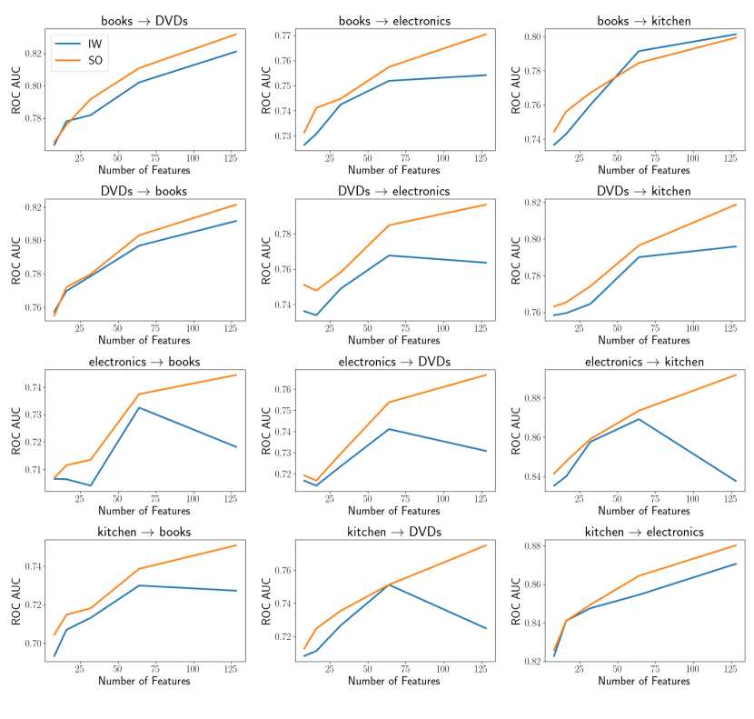
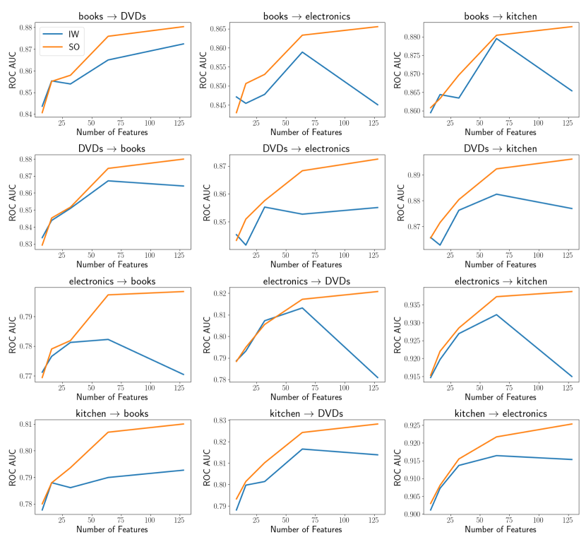
We conducted numerical experiments with real-world data to highlight important considerations in applying the proposed method. Specifically, we conducted experiments on Domain Adaptation (DA) for classification models using the Importance Weighting (IW) method [29]. The IW method builds a prediction model for a target domain using data from a source domain, while adjusting the distribution of source domain features to match the target domain features by employing the density ratio between the source and target domains as sample weights.

In these experiments, we used the Amazon review data [6] and employed two prediction algorithms: linear regression and gradient boosting. The hyperparameters for each algorithm were selected from a predefined set based on validation accuracy, using the Importance Weighted Cross Validation (IWCV) method [32] on the source domain data.

Through these experiments, we observed a decline in prediction accuracy on test data from the target domain as the data dimensionality increased. Specifically, there were instances where the accuracy worsened compared to models that did not use importance weighting—i.e., models trained solely on the source data. These phenomena are likely due to two issues in DRE: the degradation in density ratio estimation accuracy as dimensionality increases, as noted in Section E.1, and the negative impact of high KL-divergence on density ratio estimation, as observed in Section 6.3. It is important to note that the KL-divergence increases as the number of features increases (i.e., data dimensions), unless all features are fully independent.

E.2.1 Datasets.

The Amazon review dataset [6] includes text reviews and rating scores from four domains: books, DVDs, electronics, and kitchen appliances. The text reviews are one-hot encoded, and the rating scores are converted into binary labels. Twelve domain adaptation classification tasks were conducted, where each domain served once as the source domain and once as the target domain.

Notation.

𝐗Sd\mathbf{X}_{\text{S}}^{d} and 𝐗Td\mathbf{X}_{\text{T}}^{d} denote subsets of the original data for the source and target domains, respectively, for each feature dimension dd, where the columns of 𝐗Sd\mathbf{X}_{\text{S}}^{d} and 𝐗Td\mathbf{X}_{\text{T}}^{d} are identical. ySy_{\text{S}} and yTy_{\text{T}} represent the objective variables in the source and target domains, respectively, which are binary labels assigned to each sample in the source and target domain data. 𝐙Sd\mathbf{Z}_{\text{S}}^{d} and 𝐙Td\mathbf{Z}_{\text{T}}^{d} denote dd-dimensional feature tables used to estimate the density ratio r^(𝐙Sd)\hat{r}(\mathbf{Z}_{\text{S}}^{d}), which is the ratio of the target domain density to the source domain density. dim(X)\text{dim}(X) indicates the number of columns (features) in the data XX.

E.2.2 Experimental Procedure.

Step 1. Creation of feature tables.

Many DA methods utilize feature embedding techniques to project high-dimensional data into a lower-dimensional feature space, facilitating the handling of distribution shifts between source and target domains [27]. However, our preliminary experiments revealed that model prediction accuracies were significantly influenced by the embedding procedures. To address these effects on DA task accuracies, we explored an embedding method with theoretical considerations detailed in the next section.

Specifically, we selected an identical set of columns from the original data of both the source and target domains for each feature dimension, d=8,16,32,64d=8,16,32,64, and 128128, arranging the columns in ascending order of dd. Let 𝐗Sd\mathbf{X}_{\text{S}}^{d} and 𝐗Td\mathbf{X}_{\text{T}}^{d} denote the subsets of the original data for the source and target domains, respectively, determined by these selected columns for each dd. We then generated a d×dim(𝐗Sd)d\times\text{dim}(\mathbf{X}_{\text{S}}^{d}) matrix AdA_{d} from a normal distribution. Finally, by multiplying 𝐗Sd\mathbf{X}_{\text{S}}^{d} and AdA_{d}, and 𝐗Td\mathbf{X}_{\text{T}}^{d} and AdA_{d}, we obtained the feature tables 𝐙Sd\mathbf{Z}_{\text{S}}^{d} and 𝐙Td\mathbf{Z}_{\text{T}}^{d}, embedding the original source and target domain data into a dd-dimensional feature space. 333In our experiments, we utilized matrices generated from the normal distribution as embedding maps, which is equivalent to random projection [4]. However, the linearity of the map is not necessary for preserving the density ratios, as discussed in Section E.2.3. In contrast, linearity is a key requirement for the distance-preserving property of random projection.

Step 2. Estimation of importance weights.

Using the proposed loss function with 𝐙Sd\mathbf{Z}_{\text{S}}^{d} and 𝐙Td\mathbf{Z}_{\text{T}}^{d} obtained from the previous step, we estimated the probability density ratio r^(𝐙Sd)\hat{r}(\mathbf{Z}_{\text{S}}^{d}) for each feature dimension dd, where r(𝐙Sd)=q(𝐙Td)/p(𝐙Sd)r(\mathbf{Z}_{\text{S}}^{d})={q(\mathbf{Z}_{\text{T}}^{d})}/{p(\mathbf{Z}_{\text{S}}^{d})}. This ratio represents the density of the target domain relative to the source domain.

Step 3. Model construction.

We constructed the target model using the IW method. Specifically, we built a classification model using the training dataset (𝐗Sd,yS)(\mathbf{X}_{\text{S}}^{d},y_{\text{S}}), where the estimated density ratio r^(𝐙Sd)\hat{r}(\mathbf{Z}_{\text{S}}^{d}) served as the sample weights for the IW method. Additionally, we constructed a prediction model using only the source data, i.e., a model built without importance weighting.

Step 4. Verification of prediction accuracy

To evaluate the prediction accuracy of the models, we selected the ROC AUC score, as it measures the accuracy independent of the thresholds used for label determination. For the classification tasks in domain adaptation, we employed two classification methods, each representing a different algorithmic approach: LogisticRegression from the scikit-learn library [25] for linear classification, and LightGBM [16] for nonlinear classification.

The hyperparameter sets of both methods for evaluating the prediction accuracies on the target domains were selected using the IWCV method [32]. These hyperparameter sets were defined as all combinations of the values listed in Table 6 for LogisticRegression and Table 7 for LightGBM, respectively. Finally, the prediction accuracies on the target domain were assessed using the best model selected through IWCV, where the target domain data (𝐗Td,yT)(\mathbf{X}{\text{T}}^{d},y{\text{T}}) were used for the predictions.

Table 6: Hyperparameter values for LogisticRegression. “Hyperparameters” shows the hyperparameter names used in the library. Texts inside parentheses provide explanations of the parameters.
Hyperparameters Values
l1_ratio (Elastic-Net mixing parameter) 0, 0.1, 0.2, 0.3, 0.4, 0.5, 0.6, 0.7, 0.8, 0.9, and 1.0
lambda (Inverse of regularization strength) 0.0001, 0.001, 0.01, 0.05, 0.1, 0.25, 0.5, 0.75, 1, 1.5, 2, and 5
Table 7: Hyperparameter values for LightGBM. “Hyperparameters” shows the hyperparameter names used in the library. Texts inside parentheses provide explanations of the parameters.
Hyperparameters Values
lambda_l1 (L1L_{1} regularization) 0.0, 0.25, 0.5, 0.75, and 1.0
lambda_l2 (L2L_{2} regularization) 0.0, 0.0001, 0.001, 0.01, 0.1, 0.5, 1.0, 2.0, and 4.0
num_leaves (Number of leaves in trees) 64, 248, 1024, 2048, and 4096
learning_rate (Learning rate) 0.01, and 0.001
feature_fraction (Ratio of featuresr used for modeling) 0.4, 0.8, and 1.0
Table 8: Original data dimensions (dim(𝐗)\text{dim}(\mathbf{X})) used to obtain feature dimensions (dim(𝐙)\text{dim}(\mathbf{Z})) by embedding.
Feature dimensions (d=dim(𝐙)d=\text{dim}(\mathbf{Z}))
d=8d=8 d=16d=16 d=32d=32 d=64d=64 d=128d=128
Original data dimensions (dim(𝐗)\text{dim}(\mathbf{X})) 500 700 900 1700 4600

E.2.3 Consideration of the Feature Embedding Method

Let f:𝐗𝐙f:\mathbf{X}\longmapsto\mathbf{Z} denote a C1C^{1}-class embedding map which maps the original data 𝐗N×D\mathbf{X}\subseteq\mathbb{R}^{N\times D} into the feature space 𝐙N×d\mathbf{Z}\subseteq\mathbb{R}^{N\times d} with d<Dd<D.

We now demonstrate that if ff is injective for both the source and target domain data, it preserves the density ratio between the target and source domain densities when it maps the original data into the embedded data.

To demonstrate this, we use the singular value decomposition (SVD) of the Jacobian matrix Jf(𝐱)J_{f}(\mathbf{x}) of ff, which gives

Jf(𝐱)=U(𝐱)Σ(𝐱)VT(𝐱),J_{f}(\mathbf{x})=U(\mathbf{x})\cdot\Sigma(\mathbf{x})\cdot V^{T}(\mathbf{x}),

with

Σ(𝐱)=(σ1(𝐱)000σ2(𝐱)000σdim(𝐳)(𝐱)000000),\Sigma(\mathbf{x})=\begin{pmatrix}\sigma_{1}(\mathbf{x})&0&\dots&0\\ 0&\sigma_{2}(\mathbf{x})&\dots&0\\ \vdots&\vdots&\ddots&\vdots\\ 0&0&\dots&\sigma_{\text{dim}(\mathbf{z})}(\mathbf{x})\\ 0&0&\dots&0\\ \vdots&\vdots&\dots&\vdots\\ 0&0&\dots&0\\ \end{pmatrix},

where U(𝐱)U(\mathbf{x}) and VT(𝐱)V^{T}(\mathbf{x}) are orthogonal matrices in dim(𝐱)×dim(𝐱)\mathbb{R}^{\text{dim}(\mathbf{x})\times\text{dim}(\mathbf{x})} and dim(𝐳)×dim(𝐳)\mathbb{R}^{\text{dim}(\mathbf{z})\times\text{dim}(\mathbf{z})}, respectively, and σi(𝐱)0\sigma_{i}(\mathbf{x})\neq 0 for all ii. This gives the following relationship between the probability densities of the original and embedded data:

p𝐗(𝐱)=(i=1dim(𝐳)σi(𝐱))p𝐙(f(𝐱)).p_{\mathbf{X}}(\mathbf{x})=\left(\prod_{i=1}^{\text{dim}(\mathbf{z})}\sigma_{i}(\mathbf{x})\right)p_{\mathbf{Z}}(f(\mathbf{x})). (88)

From Equation (88), the probability density ratio between the source and target domains of data embedded by ff is obtained as

q𝐗(𝐱)p𝐗(𝐱)=(i=1dim(𝐳)σi(𝐱))q𝐙(f(𝐱))(i=1dim(𝐳)σi(𝐱))p𝐙(f(𝐱))=q𝐙(𝐳)p𝐙(𝐳).\frac{q_{\mathbf{X}}(\mathbf{x})}{p_{\mathbf{X}}(\mathbf{x})}=\frac{\left(\prod_{i=1}^{\text{dim}(\mathbf{z})}\sigma_{i}(\mathbf{x})\right)\cdot q_{\mathbf{Z}}(f(\mathbf{x}))}{\left(\prod_{i=1}^{\text{dim}(\mathbf{z})}\sigma_{i}(\mathbf{x})\right)\cdot p_{\mathbf{Z}}(f(\mathbf{x}))}=\frac{q_{\mathbf{Z}}(\mathbf{z})}{p_{\mathbf{Z}}(\mathbf{z})}.

Therefore, ff preserves the density ratio from the original data to the embedded data. Additionally, if ff is a matrix multiplication, its injectivity can be achieved for 𝐗\mathbf{X} by reducing its dimensionality sufficiently. Reducing the dimensionality of 𝐗\mathbf{X} can ensure the injectivity of ff.

We heuristically detected the injectivity of our embedding by observing the following: We identified the largest subset of columns in 𝐙Sd\mathbf{Z}_{\text{S}}^{d} such that a significant increase in the KL-divergence between P(𝐙Sd)P(\mathbf{Z}_{\text{S}}^{d}) and P(𝐙Td)P(\mathbf{Z}_{\text{T}}^{d}) was observed when a column is added to a partial subset of columns within it. Injectivity was assumed for columns within this subset.

Although our feature embedding procedure is based on heuristic observations and lacks rigorous theoretical analysis, we found it adequate for evaluating the performance of the proposed method in DRE downstream tasks with real-world data when the number of features increases.

The number of columns in the original data used in the experiments is listed in Table 8.

Neural Network Architecture, Optimization Algorithm, and Hyperparameters.

A 5-layer perceptron with ReLU activation was used, with each hidden layer consisting of 256 nodes. For optimization, the value of α\alpha was set to 0.5, the learning rate to 0.0001, and the batch size to 128. Early stopping was applied with a patience of 1 epoch, and the maximum number of epochs was set to 5000. The PyTorch library [24] in Python served as the framework for model implementation. Training of the neural networks was carried out using the Adam optimizer [17] on an NVIDIA T4 GPU.

Results.

The results are shown in Figure 5 (LogisticRegression) and Figure 6 (LightGBM). The domain names at the origin of the arrows in the figure titles represent the source domains, and those at the tip indicate the target domains. The xx-axis of each figure shows the number of features, and the yy-axis represents the ROC AUC for the domain adaptation tasks. The orange line (SO) represents models trained using source-only data, i.e., models trained using source data without importance weighting, while the blue line (IW) represents models trained using source data with importance weighting.

Prediction accuracy for the models trained solely on the source data improved as the number of features increased, which is expected since more features typically lead to better accuracy. However, for both Logistic Regression and LightGBM, the performance of the IW method deteriorated as the number of features increased. A more significant decline in performance with increasing features was observed for most domain adaptation (DA) tasks, except for “books \rightarrow DVDs” and “kitchen \rightarrow DVDs”. These results suggest that the estimated density ratios caused the data distribution to deviate more from the target domain as the number of features increased. Consequently, the accuracy of the density ratio estimation (DRE) likely worsened with more features.

Refer to caption

Figure 5: Results of Section E.2 for LogisticRegression. In the figure titles, domain names at the origin of the arrows indicate the source domains, while those at the tip represent the target domains. The xx-axis shows the number of features, and the yy-axis represents the ROC AUC for the domain adaptation tasks. The orange line (SO) denotes models trained using source-only data (i.e., models trained on source data only, without importance weighting), whereas the blue line (IW) represents models trained using source data with importance weighting.

Refer to caption

Figure 6: Results of Section E.2. Results of Section E.2 for LightGBM. In the figure titles, domain names at the origin of the arrows represent the source domains, while those at the tip indicate the target domains. The xx-axis shows the number of features, and the yy-axis represents the ROC AUC for the domain adaptation tasks. The orange line (SO) denotes models trained using source-only data (i.e., models trained on source data only, without importance weighting), whereas the blue line (IW) represents models trained using source data with importance weighting.