An abstract inf-sup problem inspired by limit analysis in perfect plasticity and related applications
Abstract
This work is concerned with an abstract inf-sup problem generated by a bilinear Lagrangian and convex constraints. We study the conditions that guarantee no gap between the inf-sup and related sup-inf problems. The key assumption introduced in the paper generalizes the well-known Babuška-Brezzi condition. It is based on an inf-sup condition defined for convex cones in function spaces. We also apply a regularization method convenient for solving the inf-sup problem and derive a computable majorant of the critical (inf-sup) value, which can be used in a posteriori error analysis of numerical results. Results obtained for the abstract problem are applied to continuum mechanics. In particular, examples of limit load problems and similar ones arising in classical plasticity, gradient plasticity and delamination are introduced.
Keywords: convex optimization, duality, inf-sup conditions on cones, regularization, computable majorants, plasticity, delamination, limit analysis
1 Introduction
This paper is concerned with analysis of the abstract duality problem
| (1.1) |
where is a closed, convex set with , are Banach spaces, is a non-trivial continuous linear functional in , and is a bilinear form continuous with respect to both arguments. Henceforth the problem in the right hand side of (1.1) is called primal, while the one in the left hand side is called dual. It is easy to check that . In general, necessary and sufficient conditions for are unknown (therefore, (1.1) uses the symbol ). One of our main goals is to identify cases where (1.1) holds as the equality.
Problem (1.1) and similar problems appear in various applications, from mechanics to economics [12, 9, 3]. In finite dimensions, minimax and maximin variants of these problems are known in game theory [19] and linear, cone or convex programming [11, 5, 21, 18].
In classical elastic-perfect plasticity, (1.1) is known as the limit analysis problem. In this case, is the factor that determines the critical load ( is a linear functional associated with external loads), subject to the constraint set of plastically admissible stresses; see for example [17, 9, 32, 8, 10, 29, 30, 28, 16]. For the load with , no solution of the primal and dual problems exists; the body is unable to sustain the loading and collapses. Also, we note the similarity between (1.1) and the shakedown analysis problem (see [33] and the references therein).
Although the limit analysis problem has been studied for several decades, it is still unsolved in the general setting and presents a challenging problem from the theoretical and numerical points of view. There are several reasons that stimulate further analysis of the problem. First, we notice that the equality can be analyzed in a rather general framework introduced in [12] or by using particular results from [9, 32, 16]. However, these results do not cover any interesting cases. Second, additional and hidden constraints appear in the primal and dual problems (that follow from their inf- and sup-definitions). They often make the numerical analysis difficult. The third reason is related to the choice of the function spaces and . This question becomes especially important if the primal problem is related to minimization of a functional with linear growth at infinity and a certain problem relaxation must be done to find a minimizer (see e.g. [17, 32, 29, 10]). Then we arrive, for example, at a formulation in which the - or - spaces of functions of bounded deformation and bounded variation, respectively, are appropriate for the problem setting [32]. Nevertheless, standard Sobolev spaces seem to be sufficient or even more appropriate for analysis of numerical errors [27, 28, 16]. Finally, reliable estimates of and are often required because they define safety factors of structures. Lower bounds of and upper bounds of can be found by analytical approaches for specific geometries [8] or, more generally, by finite element methods; see [30] and the references therein. Computable majorants of can be found in recent papers [28, 16].
In order to investigate the abstract problem (1.1), we use the ideas applied in [14, 15, 28, 16] for analysis of limit load problems. This extension is not always straightforward and requires innovative techniques. In particular, we derive conditions for the equality to hold, the existence of a solution to the dual problem in (1.1), a regularization method for solving (1.1) with related convergence results, and a computable majorant of , which can be used for a posteriori analysis of numerical results.
One of the key assumptions in the results presented is the so-called inf-sup condition on convex cones which was introduced in [16]. This condition generalizes the Babuška-Brezzi condition defined on function spaces [1, 4]. Conditions of this type are important for analysis of saddle point problems generated by various mixed finite element approximations [3].
Generalization and abstraction of results is a basic procedure that allows results and insights in a particular application to be applied to broad classes of problems. In our case, we show that the results presented here are useful in problems of gradient-enhanced plasticity and in delamination problems. We choose the strain gradient model studied in [25, 24, 6, 26] and use (1.1) for the description of a global yield surface and for limit load analysis. In related work, limit analysis has been considered for a model in which size-dependence is through the gradient of a scalar function of plastic strain, see [13, Section 7] or [23]. One can expect further applications of the problem (1.1), at least within nonlinear mechanics.
The rest of the paper is organized as follows. In Section 2, we introduce the primal and dual problems, discuss them in more detail, and present criteria ensuring their solvability and the principal duality relation . One of the criteria is based on the inf-sup condition on convex cones. The proof of this new result is carried out in Section 3 and its extensions are studied in Section 4. Section 5 is devoted to a regularization of the problem (1.1). The regularized problem provides a lower and sufficiently sharp bound of , reduces the constraints in the dual problem, and thus it is convenient for numerical solution. In Section 6, a computable majorant of the quantity is derived. Section 7 contains particular examples of the abstract problem (1.1), including classical and strain-gradient plasticity and a delamination problem.
2 The primal and dual problems and duality criteria
First, we recapitulate the basic assumptions used in the problem (1.1):
-
(A1)
are two Banach spaces equipped with the norms and , respectively. The corresponding dual spaces are denoted by and ;
-
(A2)
is a continuous bilinear form;
-
(A3)
is a non-trivial continuous linear functional (i.e., in );
-
(A4)
is a nonempty, closed and convex set with .
The primal problem in (1.1) reads
| (2.1) |
where
| (2.2) |
The functional is convex, proper and 1-positively homogeneous. In addition, the effective domain is a convex cone; see Section 6 for more details. We shall assume that all cones considered in the text have a vertex at zero, so henceforth do not emphasize this property. We say that the problem (2.1) has a solution if the functional has a minimizer in the feasible set . Using the positive homogeneity of , we obtain the following useful and equivalent definition of :
| (2.3) |
To rewrite the dual problem in (1.1) we define the functional
| (2.4) |
and the related set
| (2.5) |
Then, we have
| (2.6) |
We shall say that the problem (2.6) has a solution if and there exists .
Now, we present three different results ensuring the equality and the existence of primal or dual solutions. The first result follows from [12, Proposition VI.2.3 and Remark VI.2.3].
Theorem 2.1.
Let (A1)–(A4) be satisfied and assume in addition that
-
(B)
is a bounded set in .
Then and the dual problem (2.6) has a solution.
Unfortunately, the set can be unbounded in plasticity and other applications. Therefore, we also need other criteria. The second result has been introduced in [9, Theorem 2.1] and also used in [10, Theorem 5.7]. It is convenient for use with non-reflexive spaces such as .
Theorem 2.2.
Let (A1)–(A4) be satisfied together with the following:
-
has a non-empty interior in ;
-
There exists such that for any ;
-
For any such that
there exists satisfying for any .
Then and the primal problem has a solution.
The third result is inspired by [16, Theorem 5.2]. It is convenient for analysis on reflexive Banach spaces. This result is new and will be proven in the next section.
Theorem 2.3.
Let (A1)–(A4) be satisfied and, in addition, assume the following:
-
is a reflexive Banach space;
-
is a Hilbert space with a scalar product and the induced norm ;
-
For any there exist and such that , where is closed, convex and bounded and is a closed convex cone;
-
(2.7)
Then . Moreover, if then the dual problem (2.6) has a solution.
It is worth noting that for the validity of the theorem it suffices to assume that the set is only closed and convex in and satisfies . On the other hand, we have
This fact (independence of the scaling parameter) explains why we assume that is a convex cone. In addition, we shall see in Section 6 that the cones and are closely related.
3 The proof of Theorem 2.3
Within this section we assume that the conditions (A1)–(A4), (D1)–(D4) are satisfied and also (notice that Theorem 2.3 holds trivially for ). To prove this theorem we define auxiliary functions and :
| (3.1) |
Their basic properties are introduced in the following lemma.
Lemma 3.1.
The function is nonnegative, convex and Lipschitz continuous in for any . The function is nonnegative, nondecreasing, and Lipschitz continuous in .
Proof.
It is straightforward to verify that and are nonnegative and convex. Let . Then, using continuity of the bilinear form , we have
where is the norm of . Similarly, and so proving the Lipschitz continuity of in .
Since is convex and , we have for any and . Hence,
i.e, is nondecreasing in . Let , . Then and
Thus is Lipschitz continuous in with modulus . ∎
Lemma 3.2.
Proof.
To prove (3.2) we use the Lagrangian
| (3.4) |
The mapping is coercive, convex, and continuous in for any while is linear for any and the set is closed and convex in . Therefore, by [12, Proposition VI 2.3], we know that
| (3.5) |
For any given , there exists a unique element such that
or equivalently
| (3.6) |
Consequently,
| (3.7) |
and
| (3.8) |
From (3.5) and (3.8), we have:
where is the primal functional defined by (2.2). Thus,
| (3.9) |
From (2.3), one can see that for any and . Hence, for any and using the continuity argument. On the other hand, if then there exists such that . Hence,
for any small enough. From this and (3.9), it follows that for any . Therefore, (3.2) holds. It is easy to see that (3.3) follows from (3.2) and the inequality . ∎
Next, consider the following problem: given ,
| (3.10) |
Lemma 3.3.
Proof.
Proof of Theorem 2.3. The proof is based on Lemma 3.3. We show that the problem (3.10) has a solution for any under the assumptions of Theorem 2.3. From Lemma 3.1, we know that the function is convex and Lipschitz continuous in for any . Using the assumptions (D3) and (D4) we prove that is also coercive in for any . Indeed, for any and , we have:
| (3.11) | |||||
where is the inf-sup constant from (2.7) and is a positive constant characterizing the boundedness of . Since is a reflexive Banach space, the properties of guarantee that (3.10) has a solution for any . ∎
4 Generalizations of Theorem 2.3
Now we present three different generalizations (or extensions) of Theorem 2.3. Since their proofs are quite analogous, we only sketch them.
First, the assumption (D4) cannot hold if the subspace
| (4.1) |
contains an element such that . In Section 7, we will show that this case may arise in some applications. To weaken the assumption (D4) we introduce the quotient space (with the norm ) whose elements are the equivalence classes induced by the equivalence relation:
Let denote the set of equivalent classes generated by the set . It is easy to verify that is a closed, convex, and nonempty set in . Similarly, one can introduce the sets and , where and are defined in accordance with the assumption (D3). These sets have properties analogous to properties of and . In particular, for any there exists and such that . We note that if is a Hilbert space then can be identified with the orthogonal complement of in and with the projection of onto .
Theorem 4.1.
Sketch of the proof: It suffices to show that (3.10) has a solution in for any under the assumptions of this theorem. Let be fixed. Using (4.1), we see that the function defined in (3.1) satisfies
| (4.3) |
Therefore, (3.10) has a solution in if and only if has a minimum in . From (4.2), one can prove the coercivity of in analogously as in the proof of Theorem 2.3. Therefore, has a minimum in and thus the result of Theorem 4.1 holds. ∎
Second, it turns out that the assumption (D2) of Theorem 2.3 can be extended to some reflexive Banach spaces associated with a bounded Lipschitz domain , .
Theorem 4.2.
Let the assumptions (A1)–(A4) and (D1), (D3)-(D4) be satisfied and
-
(D2’)
, equipped with the standard Sobolev norm
Then . In addition, if then the dual problem (2.6) has a solution.
Sketch of the proof: It suffices to modify formulae (3.4)–(3.9). To this end, we set
| (4.4) |
Then (3.5) holds and there exists a unique element such that
or equivalently
| (4.5) |
Consequently,
| (4.6) |
and
| (4.7) |
where . The rest of the proof is analogous to that of Section 3. ∎
The third extension illustrates that Theorem 2.3 remains valid even if the space is replaced by its conic subset.
Theorem 4.3.
Let the assumptions (A1)–(A4) and (D1)–(D3) of Theorem 2.3 be satisfied, be a closed convex cone, and
| (4.8) |
Then
| (4.9) |
In addition, , where
Sketch of the proof: The following two changes in the proof of Theorem 2.3 are necessary:
-
1.
We define
and consider the minimization problem
with defined by (3.4). Since is a closed convex cone, the corresponding necessary and sufficient condition characterising reads
We obtain
so that .
- 2.
Then the proof of Theorem 2.3 is applicable without any substantial changes.
5 Regularization method
Regularization methods are often used for solving nonsmooth, constrained, or ill-posed problems. As an example, we mention proximal point methods [22] which can be used for solving the problems (2.6) and (2.1).
Here we consider another regularization method which has been subsequently developed in [31, 7, 14, 15] and used also in [28, 16]. In these recent papers, this method has been called either the “indirect incremental method” or the “penalization method”. Below, we generalize, results of [14, 15] and show that some of these can be established in a simpler way. Within this section it is assumed that the conditions (A1)–(A4) from Section 2 hold.
To regularize the functional defined by (2.2) we introduce the functional
| (5.1) |
where is a given parameter. It is easy to see that is convex and finite-valued in (unlike the functional ) and for any , .
Proof.
Let be fixed. As mentioned above, the sequence is nondecreasing. Therefore, it has a limit which is less than or equal to . On the other hand,
Thus (5.2) holds. ∎
The regularization of the primal problem (2.1) with respect to the parameter defines the function :
| (5.3) |
In view of (5.1) and [12, Proposition VI 2.3], it holds
| (5.4) |
Thus, the main duality relation holds without any gap, unlike the original primal-dual problem (1.1). The properties of the function are set out in the following theorem.
Theorem 5.1.
Proof.
From the properties of , it is easy to see that is nondecreasing and thus it has a limit as . Comparing (2.6) and (5.4)3 we see that . In addition, for any we have
Making use of the definition of , we arrive at (5.5).
Let . Since , we have if . Hence,
This relation and the monotonicity of imply
Hence,
| (5.6) |
It is worth noting that for any value of , the quantity is a lower bound of and . Upper bounds of and will be derived in the next section.
From the numerical point of view, it is useful if the functional is differentiable in the Gâteaux sense. Below we establish this property of the regularized functional.
Lemma 5.2.
Let be a Hilbert space with the scalar product and define
| (5.8) |
Then is Lipschitz continuous in and
| (5.9) |
Proof.
Since is a Hilbert space, it is easy to see that there exists a unique solving (5.8) and satisfying the variational inequality
| (5.10) |
Hence, we derive the inequalities
which hold for any and any . By adding these inequalities, we obtain
Thus is Lipschitz continuous in .
Using the differentiability of , one can rewrite the problem (5.3) as a system of nonlinear variational equations.
Theorem 5.2.
Remark 5.1.
In [14], the function was introduced and analysed for the case of Hencky plasticity. It is worth noticing that this function is well defined even if (5.3) does not have a minimizer in . In addition, is continuous and nondecreasing, with for any , and as . One can expect that these considerations from [14] can be extended to our abstract problem.
6 A computable majorant of
For classical limit analysis problems, computable majorants of have been derived in [28, 16]. The aim of this section is to derive a more general majorant valid for the abstract problem (2.1). In our analysis, we shall use the assumptions (A1)–(A4) and (D1)–(D4) of Theorem 2.3. The following alternative to the assumption (D3) will also be considered:
-
(D3′)
, where , and have the same properties as in (D3).
We note that (D3′) is more restrictive than (D3); it has been used in [16].
From the definition of (see (2.6)), we have the following simple upper bound of :
| (6.1) |
Unfortunately, if the set is unbounded then it is difficult or even impossible to find in such a way that the bound (6.1) would be sufficiently sharp. The aim of this section is to derive an upper bound of for a larger class of functions , not necessarily belonging to .
First, we need to characterize the set . For this purpose, we define the closed convex cone
| (6.2) |
and the convex, finite-valued functional
| (6.3) |
Lemma 6.1.
Let the assumptions (A1)–(A4) and (D1)–(D4) be satisfied. Then
| (6.4) |
Moreover, if (D3) holds then for any .
Proof.
From the definition of and the boundedness of and , we easily derive the useful estimates
| (6.7) |
and
| (6.8) |
In order to estimate using , it is important to measure the distance between and . Define the quantity
| (6.9) |
Remark 6.1.
It is also useful to note that if then . We have the following result.
Lemma 6.2.
Proof.
Theorem 6.1.
Let the assumptions (A1)–(A4) and (D1)–(D4) be satisfied and be such that
| (6.15) |
Then
| (6.16) |
Proof.
Remark 6.2.
Remark 6.3.
If is sufficiently close to the cone then the assumption (6.15) is satisfied. This can be achieved by a convenient numerical method, e.g., by the regularization method presented in the previous section.
Remark 6.4.
Remark 6.5.
In [28], a computable majorant of the limit load was used in the Hencky plasticity problem to prove convergence of the standard finite element method and to detect locking effects that may arise when the simplest P1 elements are used.
7 Examples
In this section, we illustrate the abstract problem (1.1) on particular examples from nonlinear mechanics and discuss the validity of the assumptions (A1)–(A4), (B) and (D1)–(D4) presented in Section 2. In all examples we consider a bounded domain , , with Lipschitz continuous boundary . The outward unit normal to is denoted by . The abstract spaces and will be represented by and spaces, respectively, for the sake of simplicity.
7.1 Limit analysis in classical perfect plasticity
Details of the mathematical theory of limit analysis in classical perfect plasticity may be found in [32] or [10]. For its engineering applications we refer, for example, to [8, 30]. The aim is to find the largest load factor at which plastic behaviour may be sustained, in the context of proportional loading. We briefly recapitulate results presented in [16, 28, 15, 14].
A body occupying the domain is fixed on a part and surface forces act on the remaining part of . We assume that and have a positive surface measure. Let denote the volume force. The external loads are parametrized by a scalar factor .
Next, we denote the space of symmetric matrices (second order tensors) by . The Cauchy stress field satisfies the equilibrium equation and traction boundary condition
| (7.1a) | ||||
| (7.1b) | ||||
and is plastically admissible in the sense that
| (7.2) |
Here, , , is a convex function representing a yield criterion. For the sake of simplicity, we assume that and thus are independent of the spatial variable.
The infinitesimal strain rate and the displacement rate satisfy the relations
| (7.3) |
The last ingredient of the perfectly plastic model is a plastic flow rule that relates and , and which is based on the set . This relation is represented by the principle of maximum plastic dissipation in quasistatic models or by a generalized projection of onto in total strain models. We skip its definition, for the sake of brevity.
Formally, the limit load factor is defined as the supremum over subject to (7.1a), (7.1b) and (7.2). To define more precisely and in the form (2.6), it is necessary to introduce a convenient function space for stress fields. For this purpose define the Hilbert space
equipped with the scalar product and norm
where with the summation convention on repeated indices. The corresponding primal space is chosen as follows:
It is also a Hilbert space representing rates of displacements with the following scalar product and norm:
Using the spaces and Green’s theorem, a weak formulation of (7.1a) and (7.1b) for fixed reads as follows:
| (7.4) |
where
| (7.5) |
with , and . It is easy to see that is a continuous bilinear form in and . Using the notation from Section 1, one can write
where
| (7.6) |
The sets and are closed, convex and non-empty in and represent plastically and statically admissible stresses, respectively.
We note that the set is defined in a pointwise sense. Consequently, the sets , and the functions , , and introduced in the previous sections may be also defined in a pointwise sense. To illustrate, we choose the von Mises yield criterion defined by
| (7.7) |
where is the unit matrix, denotes the trace of , is the deviatoric part of and is a given parameter representing the initial yield stress. From [32, 10, 16], it is known that can be decomposed according to , where
Clearly, is bounded in and is a closed subspace of , that is, a convex cone. To prove (2.7), we use the well-known inf-sup condition for incompressible flow media with :
| (7.8) |
Thus, the condition (2.7) holds with . Consequently, the assumptions (A1)–(A4), (D1)–(D4) from Section 2 are satisfied and from Theorem 2.3 it follows that
Notice that if then it is necessary to use Theorem 4.1 with the weaker assumption (4.2) instead of (D4). In this case, we replace the space in (7.8) by , see [28, 16].
The primal functional for the von Mises yield criterion is given by
This functional may have no minimizers in . To guarantee that the primal problem is solvable, it is necessary to use another choice of and , as was done, for example, in [9, 32, 10]. In particular, the assumptions (C1)–(C3) of Theorem 2.2 were verified in [9, 10].
The functions , and for the von Mises yield criterion can be found in the following forms:
Let us recall that they are important for the regularization method and the computable majorant presented in the previous sections. We refer to [14, 15, 28, 16] for more details.
Remark 7.1.
If we choose the Drucker-Prager or Mohr-Coulomb yield criteria in (7.2) instead of von Mises then it is also possible to find an appropriate split such that the assumptions (D3) and even (D3′) are satisfied. But for these criteria the cone is not a subspace of . Therefore, it is necessary to work with the inf-sup condition on convex cones, see [16].
7.2 Plastically admissible stresses in strain-gradient plasticity
In the next two subsections, we consider as further examples the models of strain-gradient plasticity presented in [25, 24, 6, 26]. First, following [26], we introduce a subproblem that enables us to decide whether a given stress tensor is plastically admissible or not. We note that this problem is simple in classical plasticity where the yield criterion can be verified pointwisely (see, for example the definition of in (7.6)). However, plastic yield criteria in strain-gradient plasticity are non-local and the verification is strongly non-trivial.
Beside the space defined in Section 7.1, we also use the following spaces of the second and third order tensors, respectively:
Thus, the third order tensor belongs to if it is symmetric and deviatoric with respect to the first two indices.
We assume that is a given stress field and denotes its deviatoric part. The theory of strain gradient plasticity makes use of second- and third-order tensors and that represent microstresses. We say that is plastically admissible if there exists a pair such that
| (7.9) |
| (7.10) |
where is the yield stress, is the length parameter, and . The part of complementary to in is denoted by .
We note that the yield criterion (7.10) can be viewed as an extension of the classical condition (7.7). Indeed, setting we derive the sufficient condition for to be plastically admissible. Unlike the classical case, the stress can be plastically admissible even if .
If is plastically admissible then is also plastically admissible for any . This parametrization motivates us to introduce the following problem: find the maximal value of for which is plastically admissible in the sense of (7.9) and (7.10). Clearly, if then is admissible.
Let us define more precisely, using the abstract problem (2.6). We assume that all components of , and belong to , that is, , and . The space is defined as the space of pairs endowed with the scalar product
The primal space
is the Hilbert space of admissible plastic strain rates with the scalar product
Using the spaces and , we introduce the following weak form of (7.9):
| (7.11) |
and define the forms and by
Then the dual problem (2.6) reads
where
From (7.10), it follows that is bounded in , i.e. the assumption (B) of Theorem 2.1 is satisfied. Thus we have
In this case, the functional can be found in the form
Although is finite-valued everywhere, it is not coercive in . Therefore, a certain relaxation of the problem is necessary if we wish to properly define a minimizer of and guarantee its existence. Such an analysis has not been done for this problem and we leave this as a topic for further investigation.
The primal and dual problems have been solved by regularization (penalization) methods in [26]. In particular, the regularized functional defined by (5.1) takes the form
Reliable lower and upper bounds of have also been estimated in [26] using the regularization methods.
Remark 7.2.
7.3 Limit (load) analysis in strain-gradient plasticity
Limit analysis in gradient-enhanced plasticity has been studied in [13, 23] for a model in which size-dependence is through the gradient of a scalar function of the plastic strain. Here, we consider the model from [25, 24, 6, 26] where the gradient is applied to the entire plastic strain.
We use the same tensors , , and external forces and as in Sections 7.1 and 7.2. Let us note that the pair of boundaries defined in Section 7.2 may differ from introduced in Section 7.1. The limit analysis problem for the strain gradient plasticity reads: find the supremum over all for which there exist , , such that
| (7.14) |
| (7.15) |
| (7.16) |
We see that (7.14) coincides with (7.1a) and (7.1b) from Section 7.1. However, we now use the definition of plastically admissible stresses from Section 7.2 (see (7.15) and (7.16)) instead of (7.10).
To rewrite this problem in the form (2.6) or (2.1), we split as follows:
| (7.17) |
We denote by the -space of all admissible triples . The equations (7.14) and (7.15) can be rewritten using (7.17) to the following weak form:
where
and
The space is equipped with the standard norm denoted by . The set remains the same as in (2.5) and the set of plastically admissible stresses reads
Thus, we can define the limit analysis problem as follows:
For analysis of the primal problem (2.1), it is convenient to use the split , where
It is easy to check that is bounded in and is a closed linear subspace of . We have
where
7.4 Limit analysis for a delamination problem
The last example is devoted to a model for delamination, inspired by [2]. Let denote the domain occupied by an elastic body, with boundary . The body is a laminated composite, comprising two distinct materials. The geometry is idealized with one material, referred to as the bulk, comprising the entire domain with the exception of a thin layer of the second material. This thin layer is treated as a line , and separation or delamination may occur along this line.
We follow [2] and consider a problem with a symmetric geometry and loading, as shown in Figure 1(a). Zero displacements in the normal () direction are prescribed along the boundary , while on a surface force is applied, where is a load factor. The remainder of the boundary is unconstrained and traction-free. The surface force as well as a body force act symmetrically along the axis so that , the same applying to .
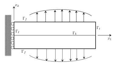
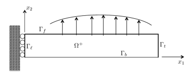
(a) (b)
Given the symmetry of the problem we may confine attention to the upper half of the domain, shown in Figure 1(b).
The boundary conditions set out above have to be augmented with a condition along . This takes the form of conditions on the traction vector : from symmetry the tangential component must be zero. Here and henceforth subscripts and refer respectively to normal and tangential components. The condition in the normal direction is a constitutive relation that (in the original domain) gives the normal traction as a function of the separation between the upper and lower surfaces along . Here is the displacement in the normal direction and denotes the jump in displacement at the interface. For the symmetrized problem one may replace the jump by . This has to be supplemented by a non-interpenetration condition, which we do not impose for now, but return to later.
The boundary conditions on are then as follows:
| (7.19) |
where denotes a multivalued step function in . Examples of can be found in [2]. For purposes of this paper, we shall assume that the values of belong to the interval where is a prescribed threshold for delamination. Then can be either the projection of onto or the multifunction for and .
The bulk material is modelled as linear elastic, to which we add the equilibrium equation on :
| (7.20) |
The limit load for the problem can be defined formally as follows: find the supremum over all for which there exists a stress field that satisfies (7.20) and
| (7.21) |
To rewrite this problem in the form (2.6) and (2.1), we introduce an auxiliary variable that coincides with on in a weak sense. Then the space contains pairs and
consists of admissible displacement fields. Using the spaces and one can rewrite the equations in (7.20)–(7.21) in the following weak form:
where
and
The set and its decomposition into and are defined as follows:
We also define . Then, the dual and primal problems read
| (7.22) |
and
| (7.23) |
To show that we use Theorem 4.1. In particular, we have
and
The latter identity follows, for example, from [20]. Then the inf-sup condition (4.2) is a consequence of the Korn inequality [20].
In addition, if then one can find analytical solutions and to (7.23) and (7.22), respectively. Indeed, from (2.2), (6.2) and Lemma 6.1, it follows that
that is, . It is readily seen that the feasible set in (7.23) is the singleton consisting of the function
provided that . If it is so then is also the unique solution to the primal problem (7.23) and
By analysis of the saddle-point problem related to (7.23) and (7.22), we find that the solution to the dual problem (7.22) satisfies and
| (7.24) |
The component is not uniquely defined. One of satisfying (7.24) is the elastic stress of the form in , where and is the elastic fourth order tensor representing Hooke’s law. If then .
Remark 7.4.
If we consider the case in which the body is fixed on as in [2], then , which implies that . Thus the related delamination problem may have a solution even if the composite is completely debonded.
Remark 7.5.
The complete formulation of the delamination problem requires also a condition of non-interpenetration (that is, a Signorini condition) along . For the symmetrized problem this amounts to defining the conic set of admissible displacement fields, replacing the last of equations (7.21) with
and consequently, replacing with . According to Theorem 4.3, we have the duality problem
By combining Theorems 4.1 and 4.3 it is possible to show that . In particular, if
we obtain the same limit value and the primal and dual solutions as for the duality problem without the non-penetration condition.
8 Conclusion
This work has been concerned with an inf-sup problem posed on abstract Banach spaces. The main feature of this convex and constrained problem has been the presence of a bilinear Lagrangian, which appears in applications leading to linear, cone or convex programming problems. Conditions for ensuring duality without any gap have been introduced. We have introduced and extended an innovative framework based on an inf-sup condition on convex cones generalizing the well-known Babuška-Brezzi conditions. We have also suggested a new regularization method and derived a computable majorant to the problem.
Applications of the abstract problem to various examples in mechanics have been presented. First, the problem of limit analysis in classical plasticity has been revisited in the context of the duality framework of this work. Then, we have shown that the abstract framework may be used in the case of two different subproblems related to strain-gradient plasticity, viz. the determination of plastically admissible stresses and the determination of limit loads, and for a delamination problem.
The techniques presented in this paper could be extended to more general duality problems where the Lagrangian contains, in addition to the bilinear form, linear forms with respect to primal or dual variables. Such an extension would be applicable to a wider range of problems in mechanics.
Acknowledgment: SS and JH acknowledge support for their work from the Czech Science Foundation (GAČR) through project No. 19-11441S. BDR acknowledges support for his work from the National Research Foundation, through the South African Chair in Computational Mechanics, SARChI Grant 47584.
References
- [1] Babuška, I. (1971). Error-bounds for finite element method. Numerische Mathematik, 16(4), 322–333.
- [2] Baniotopoulos, C.C., Haslinger, J., Morávková, Z. (2005). Mathematical modeling of delamination and nonmonotone friction problems by hemivariational inequalities. Applications of Mathematics, 50(1), 1–25.
- [3] Boffi, D., Brezzi, F., Fortin, M. (2013). Mixed Finite Element Methods and Applications. Springer.
- [4] Brezzi, F. (1974). On the existence, uniqueness and approximation of saddle-point problems arising from Lagrangian multipliers. Publications mathématiques et informatique de Rennes, (S4), 1–26.
- [5] Boyd, S. and Vandenberghe, L. (2004). Convex programming. Cambridge University Press.
- [6] Carstensen, C., Ebobisse, F., McBride, A.T., Reddy, B.D., Steinmann, P. (2017). Some properties of the dissipative model of strain-gradient plasticity. Phil. Mag. 97 (10), 693–717.
- [7] Cermak, M., Haslinger, J., Kozubek, T., Sysala, S. (2015). Discretization and numerical realization of contact problems for elastic‐perfectly plastic bodies. PART II–numerical realization, limit analysis. ZAMM‐Journal of Applied Mathematics and Mechanics/Zeitschrift für Angewandte Mathematik und Mechanik, 95(12), 1348–1371.
- [8] Chen, W. and Liu, X.L. (1990). Limit Analysis in Soil Mechanics. Elsevier.
- [9] Christiansen, E. (1980). Limit analysis in plasticity as a mathematical programming problem. Calcolo 17, 41–65.
- [10] Christiansen, E. (1996). Limit analysis of colapse states. In P. G. Ciarlet and J. L. Lions, editors, Handbook of Numerical Analysis, Vol IV, Part 2, North-Holland, 195–312.
- [11] Dantzig, G.B. (1998). Linear programming and extensions (Vol. 48). Princeton university press.
- [12] Ekeland, I. and Temam, R. (1974). Analyse Convexe et Problèmes Variationnels. Dunod, Gauthier Villars, Paris.
- [13] Fleck, N.A. and Willis, J.R. (2009). A mathematical basis for strain-gradient plasticity theory. part II: tensorial plastic multiplier. J. Mech. Phys. Solids 57, 1045–1057.
- [14] Haslinger, J., Repin, S., Sysala, S. (2016). A reliable incremental method of computing the limit load in deformation plasticity based on compliance: Continuous and discrete setting. Journal of Computational and Applied Mathematics 303, 156–170.
- [15] Haslinger, J., Repin, S., Sysala, S (2016). Guaranteed and computable bounds of the limit load for variational problems with linear growth energy functionals. Applications of Mathematics 61, 527–564.
- [16] Haslinger, J., Repin, S., Sysala, S. (2019). Inf-sup conditions on convex cones and applications to limit load analysis. Mathematics and Mechanics of Solids 24, 3331–3353.
- [17] Johnson, C. (1976). Existence theorems for plasticity problem. J. Math. Pures et Appl., 55, 79–84.
- [18] Kanno, Y. (2011). Nonsmooth mechanics and convex optimization. Crc Press.
- [19] Myerson, R.B. (2013). Game theory. Harvard university press.
- [20] Nečas, J. and Hlaváček, I. (2017). Mathematical theory of elastic and elasto-plastic bodies: an introduction, Elsevier.
- [21] Nocedal, J., and Wright, S. (2006). Numerical optimization. Springer Science & Business Media.
- [22] Parikh, N. and Boyd, S. (2014). Proximal Algorithms. Foundations and Trends in Optimization, 1(3), 127–239.
- [23] Polizzotto, C. (2010). Strain gradient plasticity, strengthening effects and plastic limit analysis. International journal of solids and structures, 47(1), 100–112.
- [24] Reddy, B.D. (2011). The role of dissipation and defect energy in variational formulations of problems in strain- gradient plasticity. Part 1: single-crystal plasticity. Cont. Mech. Thermodyn. 23, 551–572.
- [25] Reddy, B.D., Ebobisse, F., McBride, A.T. (2008). Well-posedness of a model of strain gradient plasticity for plastically irrotational materials, Int. J. Plast. 24, 55–73.
- [26] Reddy, B.D. and Sysala, S. (2020). Bounds on the elastic threshold for problems of dissipative strain-gradient plasticity. Journal of the Mechanics and Physics of Solids, 10.1016/j.jmps.2020.104089.
- [27] Repin, S. (2010). Estimates of deviations from exact solutions of variational problems with linear growth functional. Journal of Mathematical Sciences 166, 75–85.
- [28] Repin, S., Sysala, S., Haslinger, J. Computable majorants of the limit load in Hencky’s plasticity problems. Comp. & Math. with Appl. (2018) 75: 199–217.
- [29] Repin, S. and Seregin, G. (1995). Existence of a weak solution of the minimax problem arising in Coulomb-Mohr plasticity, Nonlinear evolution equations, 189–220, Amer. Math. Soc. Transl. (2), 164, Amer. Math. Soc., Providence, RI.
- [30] Sloan SW (2013). Geotechnical stability analysis, Géotechnique, 63, 531–572.
- [31] Sysala, S., Haslinger, J., Hlaváček, I., Cermak, M. (2015). Discretization and numerical realization of contact problems for elastic‐perfectly plastic bodies. PART I–discretization, limit analysis. ZAMM‐Journal of Applied Mathematics and Mechanics/Zeitschrift für Angewandte Mathematik und Mechanik, 95(4), 333–353.
- [32] Temam, R. (1985). Mathematical Problems in Plasticity. Gauthier-Villars, Paris.
- [33] Zouain, N. (2018). Shakedown and safety assessment. In: Encyclopedia of Computational Mechanics Second Edition (E. Stein, R. de Borst and T.J.R. Hughes eds.), 1–48.