An algorithm for constrained one-step inversion of spectral CT data
Abstract
We develop a primal-dual algorithm that allows for one-step inversion of spectral CT transmission photon counts data to a basis map decomposition. The algorithm allows for image constraints to be enforced on the basis maps during the inversion. The derivation of the algorithm makes use of a local upper bounding quadratic approximation to generate descent steps for non-convex spectral CT data discrepancy terms, combined with a new convex-concave optimization algorithm. Convergence of the algorithm is demonstrated on simulated spectral CT data. Simulations with noise and anthropomorphic phantoms show examples of how to employ the constrained one-step algorithm for spectral CT data.
I Introduction
The recent research activity in photon-counting detectors has motivated a resurgence in the investigation of spectral computed tomography (CT). Photon-counting detectors detect individual X-ray quanta and the electronic pulse signal generated by these quanta has a peak amplitude proportional to the photon energy [1]. Thresholding these amplitudes allows for coarse energy resolution of the X-ray photons, and the transmitted flux of X-ray photons can be measured simultaneously in a number of energy windows. Theoretically, the energy-windowed transmission measurements can be exploited to reconstruct quantitatively the X-ray attenuation map of the subject being scanned [2]. The potential benefits are reduction of beam-hardening artifacts, and improved contrast-to-noise ratio (CNR), signal-to-noise ratio (SNR), and quantitative imaging [1, 3, 4, 5]. For photon-counting detectors where the number of energy windows can be three or greater, the new advantage with respect to quantitative imaging is the ability to image contrast agents that possess a K-edge in the diagnostic X-ray energy range [6, 7, 8, 9, 10, 11].
Use of energy information in X-ray CT has been proposed almost since the conception of CT itself [12]. Dual-energy CT acquires transmission intensity at either two energy windows or for two different X-ray source spectra. Despite the extremely coarse energy-resolution, the technique is effective because for many materials only two physical processes, photo-electric effect and Compton scattering, dominate X-ray attenuation in the diagnostic energy range [2]. Within the context of dual-energy, the processing methods of energy-windowed intensity data have been classified in two broad categories: pre-reconstruction and post-reconstruction [13]. The majority of processing methods for multi-window data also fall into these categories.
In pre-reconstruction processing of the multi-energy data, the X-ray attenuation map is expressed as a sum of terms based on physical process or basis materials [2]. The multi-energy data are converted to sinograms of the basis maps, then any image reconstruction technique can be employed to invert these sinograms. The basis maps can subsequently be combined to obtain images of other desired quantities: estimated X-ray attenuation maps at a single energy, material maps, atomic number, or electron density maps. The main advantage of pre-reconstruction processing is that beam-hardening artifacts can be avoided, because consistent sinograms of the basis maps are estimated prior to image reconstruction. Two major challenges for pre-reconstruction methods are the need to calibrate the spectral transmission model and to acquire registered projections. Photon-counting detectors ease the implementation of projection registration, because multiple energy-thresholding circuits can operate on the same detection element signal. Accounting for detection physics and spectral calibration by data pre-processing or incorporation directly in the image reconstruction algorithm remains a challenge for photon-counting detectors [1].
For post-reconstruction processing, the energy-windowed transmission data are processed by the standard negative logarithm to obtain approximate sinograms of a weighted energy-averaged attenuation map followed by standard image reconstruction. The resulting images can be combined to obtain approximate estimates of images of the same physical quantities as mentioned for the pre-reconstruction processing [14]. The advantage of post-reconstruction processing is that it is relatively simple, because it is only a small modification on how standard CT data are processed and there is no requirement of projection registration. The down-side, however, is that the images corresponding to each energy-window are susceptible to beam-hardening artifacts because the negative logarithm processed data will, in general, not be consistent with the projection of any object.
A third option for the processing of spectral CT data, however, does exist, which due to difficulties arising from the nonlinearity of the attenuation of polychromatic X-rays when passing through an object, is much less common than either pre- or post-reconstruction methods: direct estimation of basis maps from energy-windowed transmission data. This approach, labeled the one-step approach in the remainder of the article, has the advantages that the spectral transmission model is treated exactly, there is no need for registered projections, and constraints on the basis maps can be incorporated together with the fitting of the spectral CT data. The main difficulty of the one-step approach is that it necessitates an iterative algorithm because the corresponding transmission data model is too complex for analytic solution, at present. Iterative image reconstruction (IIR) has been applied to spectral CT in order to address the added complexity of the data model [15, 16, 17, 18, 19, 20, 21, 22].
In this work, we develop a framework that addresses one-step image reconstruction in spectral CT allowing for non-smooth convex constraints to be applied to the basis maps. We demonstrate the algorithm with the use of total variation (TV) constraints, but the framework allows for other constraints such as non-negativity, upper bounds, and sum bounds applied to either the basis maps or to a composite image such as an estimated mono-chromatic attenuation map.
We draw upon recent developments in large-scale first-order algorithms and adapt them to incorporate the non-linear model for spectral CT to optimize the data-fidelity of the estimated image by minimizing the discrepancy between the observed and estimated data. We present an algorithm framework for constrained optimization, deriving algorithms for minimizing the data discrepancy based on least-squares fitting and on a transmission Poisson likelihood model. As previously mentioned, the framework admits many convex constraints that can be exploited to stabilize image reconstruction from spectral CT data. Section II presents the constrained optimization for one-step spectral CT image reconstruction; Sec. III presents a convex-concave primal-dual algorithm that addresses the non-convex data discrepancy term arising from the non-linear spectral CT data model; and Sec. IV demonstrates the proposed algorithm with simulated spectral CT transmission data.
II One-step image reconstruction for spectral CT
II-A Spectral CT data model
For the present work, we employ a basic spectral model for the energy-windowed transmitted X-ray intensity along a ray , where the transmitted X-ray intensity in the energy window for ray is given by
Here denotes that we are integrating along the ray while integrates over the range of energy; is the product of the X-ray beam spectrum intensity and detector sensitivity for the energy window and transmission ray at energy ; and is the linear X-ray attenuation coefficient for energy at the spatial location . Let be the transmitted intensity in the setting where no object is present between the X-ray beam and the detector (i.e. attenuation is set to zero), given by
Then we can write
| (1) |
where represents the normalized energy distribution of X-ray intensity and detector sensitivity. Image reconstruction for spectral CT aims to recovery the a complete energy-dependent linear attenuation map from intensity measurements in all windows and rays comprising the X-ray projection data set.
Throughout the article we use the convention that is the dimension of the discrete index . For example, the spectral CT data set consists of energy windows and transmission rays.
This inverse problem is simplified by exploiting the fact that the energy-dependence of the X-ray attenuation coefficient can be represented efficiently by a low-dimensional expansion. For the present work, we employ the basis material expansion
| (2) |
where is the density of material ; the X-ray mass attenuation coefficient are available from the national institute of standards and technology (NIST) report by Hubbell and Seltzer [23]; and is the fractional density map of material at location . For the present spectral CT image reconstruction problem, we aim to recover , which we refer to as the material maps.
Proceeding with the spectral CT model, we discretize the material maps by use of an expansion set
where are the representation functions for the material maps, respectively. For the 2D/3D image representation standard pixels/voxels are employed, that is, indexes the pixels/voxels. With the spatial expansion set, the line integration over the material maps is represented by a matrix with entry measuring the length of the intersection between ray and pixel :
where formally we can calculate
This integration results in the standard line-intersection method for the pixel/voxel basis.
The discretization of the integration over energy in Eq. (1) is perform by use of a Riemann sum approximation.
| (3) |
where indexes the discretized energy and
With the Riemann sum approximation we normalize the discrete window spectra,
Modeling photon-counting detection, we express X-ray incident and transmitted spectral fluence in terms of numbers of photons per ray (as before, the ray identifies the source detector-bin combinations) and energy window :
| (4) |
where is the incident spectral fluence and is interpreted as a mean transmitted fluence. Note that in general the right hand side of Eq. (4) evaluates to a non-integer value and as a result the left hand side variable cannot be assigned to an integer as would be implied by reporting transmitted fluence in terms of numbers of photons. This inconsistency is rectified by interpreting the left hand side variable, , as an expected value.
II-B Constrained optimization for one-step basis decomposition
For the purpose of developing one-step image reconstruction of the basis material maps from transmission counts data, we formulate a constrained optimization involving minimization of a non-convex data-discrepancy objective function subject to convex constraints. The optimization problem of interest takes the following form
| (5) |
where are the measured counts in energy window and ray ; is a generic data discrepancy objective function; and the indicator functions enforce the convex constraints , the are convex sets corresponding to the desired constraints (for instance, nonnegativity of the material maps). The indicator function is defined
| (6) |
Use of constrained optimization with TV constraints is demonstrated in Sec. IV.
Data discrepancy functions
For the present work, we consider two data discrepancy functions: transmission Poisson likelihood (TPL) and least-squares (LSQ)
| (7) | ||||
| (8) |
The TPL data discrepancy function is derived from the negative log likelihood of a stochastic model of the counts data
that is, minimizing is equivalent to maximizing the likelihood. Note that in defining we have subtracted a term independent of from the negative log likelihood so that is zero when , and positive otherwise. From a physics perspective, the important difference between these two data discrepancy functions is how they each weight the individual measurements; the LSQ function treats all measurements equally while the TPL function gives greater weight to higher count measurements. We point out this property to emphasize that the TPL data discrepancy can be useful even when there are data inconsistencies due to other physical factors besides the stochastic nature of the counts measurement. This alternate weighting is also achieved without introducing additional parameters as would be the case for a weighted quadratic data discrepancy. From a mathematics perspective, both data functions are convex functions of , but they are non-convex functions of . It is the non-convexity with respect to that drives the main theoretical and algorithmic development of this work. Although we consider only these two data fidelities, the same methods can be applied to other functions.
Convex constraints
The present algorithm framework allows for convex constraints that may improve reconstruction of the basis material maps. In Eq. (5) the constraints are coded with indicator functions, but here we express the constraints by the inequalities that define the convex set to which the material maps are restricted. When the basis materials are identical to the materials actually present in the subject, the basis maps can be highly constrained. Physically, the fractional densities represented by each material map must take on a value between zero and one, and the corresponding constraint is
| (9) |
Similarly, the sum of the fractional densities cannot be greater than one, leading to a constraint on the sum of material maps
| (10) |
Care must be taken, however, in using these bound and sum constraints when the basis materials used for computation are not the same as the materials actually present in the scanned object. The bounds on the material maps and their sum must likely be loosened, and therefore they may not be as effective.
In medical imaging, where multiple soft tissues comprise the subject, it is standard to employ a spectral CT materials basis which does not include many of the tissue/density combinations present. The reason for this is that soft tissues such as muscle, fat, brain, blood, etc., all have attenuation curves similar to water, and recovering each of these soft tissues individually becomes an extremely ill-posed inverse problem. For spectral CT, it is common to employ a two-material expansion set, such as bone and water, and possibly a third material for representing contrast agent that has a K-edge in the diagnostic X-ray energy range. The displayed image can then be the basis material maps or the estimated X-ray attenuation map for a single energy , also known as a monochromatic image
| (11) |
A non-negativity constraint can be applied to the monochromatic image
at one or more energies. This constraint makes physical sense even when the basis materials are not the same as the materials in the subject.
Finally, we formulate -norm constraints on the gradient magnitude images, also known as the total variation, in order to encourage gradient magnitude sparsity in either the basis material maps or the monochromatic image. In applying TV constraints to the basis material maps, we allow for different constraint values for each material
where represents the finite-differencing approximation to the gradient, and we use to represent a spatial magnitude operator so that is the gradient magnitude image (GMI) of material map . Similarly, a TV constraint can be formulated so that it applies to the monochromatic image at energy
where the constraint can be applied at one or more values of .
III A first-order algorithm for spectral CT constrained optimization
The proposed algorithm derives from the primal-dual algorithm of Chambolle and Pock (CP) [25, 26, 27]. Considering the general constrained optimization form in Eq. (5), the second term coding the convex constraints can be treated in the same way as shown in Refs. [28, 29]. The main algorithmic development, presented here, is the generalization and adaptation of CP’s primal-dual algorithm to the minimization of the data discrepancy term, the first term of Eq. (5). We derive the data fidelity steps specifically focusing on the deriving steps for and .
Optimizing the spectral CT data fidelity
We first sketch the main developments of the algorithm for minimizing the non-convex data discrepancy terms, and then explain each step in detail. The overall design of the algorithm is comprised of two nested iteration loops. The outer iteration loop involves derivation of a convex quadratic upper bound to the local quadratic Taylor expansion about the current estimate for the material maps. The inner iteration loop takes descent steps for the current quadratic upper bound. Although the algorithm construction formally involves two nested iteration loops, in practice the number of inner loop iterations is set to one. Thus, effectively the algorithm consists only of a single iteration loop where a re-expansion of the data discrepancy term is performed at every iteration.
The local convex quadratic upper bound, used to generate descent steps for the non-convex data discrepancy terms, does not fit directly with the generic primal-dual optimization form used by CP. A convex-concave generalization to the CP primal-dual algorithm is needed. The resulting algorithm called mirrored convex-concave (MOCCA) algorithm is presented in detail in Ref. [30]. For the one-step spectral CT image reconstruction algorithm we present: the local convex quadratic upper bound, a short description of MOCCA and its application in the present context, preconditioning, and convergence checks for the spectral CT image reconstruction algorithm.
III-A A local convex quadratic upper bound to the spectral CT data discrepancy terms
III-A1 Quadratic expansion
We carry out the deriviations on and in parallel. The local quadratic expansion for each of these data discrepancy terms about the material maps is
| (12) | ||||
| where | ||||
To obtain the desired expansions, we need expressions for the gradient and Hessian of each data discrepancy. The gradient of is derived explicitly in Appendix A; we do not show the details for the other derivations. The data discrepancy gradients are:
| (13) | ||||
| (14) |
where and denote the residuals in terms of counts or log counts:
| (15) | ||||
| (16) |
represents the combined linear transform that accepts material maps, performs projection, and then combines the resulting sinograms to form monochromatic sinograms at energy :
| (17) |
and is a term that results from the gradient of the logarithm of the estimated counts :
| (18) | ||||
Using the same variable and linear transform definitions, the expressions for the two Hessians are
| (19) | ||||
| (20) |
Substituting either Eq. (19) or (20) for the Hessian and either Eq. (13) or (14) for the gradient into the Taylor expansion in Eq. (12), yields the quadratic approximation to the data discrepancy terms of interest. This quadratic is in general non-convex because both Hessian expressions can have negative values.
III-A2 A local convex upper bound to
The key to deriving a local convex upper bound to the quadratic expansion of is to split the Hessian expressions into positive and negative components. Setting the negative components to zero and substituting this thresholded Hessian into the Taylor’s expansion, yields a quadratic term with non-negative curvature. (As an aside, a tighter convex local quadratic upper bound would be attained by diagonalizing the Hessian and forming a positive semi-definite Hessian by keeping eigenvectors corresponding to only non-negative eigenvalues in the eigenvalue decomposition, but for realistic sized tomography configurations such an eigenvalue decomposition is impractical.) The algebraic steps for splitting the Hessian into positive and negative components in the form
where and are both positive semidefinite (see Appendix B for more details). The resulting split expressions are:
| (21) | ||||
| (22) |
and
| (23) | ||||
| (24) |
where
and similarly
To summarize, the expression for the convex local upper bound to the quadratic approximation in Eq. (12) is
| (25) |
where is used instead of in the quadratic term. Here depends parametrically on the counts data , through the function (see Eq. (12)), and the expansion center . The gradients of at are obtained from Eqs. (13) and (14), and the Hessian upper bounds are available from Eqs. (21) and (23). Note that the quadratic expression in Eq. (25) is not necessarily an upper bound of the data discrepancy functions, even locally, because we bound only the quadratic expansion. We employ the convex function combined with convex constraints to generate descent steps for the generic non-convex optimization problem specified in Eq. (5).
III-B The motivation and application of MOCCA
III-B1 Summary of the Chambolle-Pock (CP) primal-dual framework
The generic convex optimization addressed in Ref. [25] is
| (26) |
where and are convex, possibly non-smooth, functions and is a matrix multiplying the vector . The ability to handle non-smooth convex functions is key for addressing the convex constraints of Eq. (5). In the primal-dual picture this minimization is embedded in a larger saddle point problem
| (27) |
using the Legendre transform or convex conjugation
| (28) |
and the fact that
| (29) |
if is a convex function. The CP primal-dual algorithm of interest solves Eq. (27) by iterating on the following steps
| (30) | ||||
| (31) | ||||
| (32) |
where is the iteration index; and are the primal and dual step sizes, respectively, and these step sizes must satisfy the inequality
where is the largest singular value of . Because this algorithm solves the saddle point problem, Eq. (27), one obtains the solution to the primal problem, Eq. (26) along with its Fenchel dual
| (33) |
The fact that both Eqs. (26) and (33) are solved simultaneously provides a convergence check: the primal-dual gap, the difference between the objective functions of Eqs. (26) and (33), tends to zero as the iteration number increases.
In some settings, the requirement may be impractical or too conservative, and the CP algorithm can instead be implemented with diagonal matrices and in place of and [26], with the condition and the revised steps
| (34) | ||||
| (35) | ||||
| (36) |
where for a positive semidefinite matrix the norm is defined as .
III-B2 The need to generalize the CP primal-dual framework
To apply the CP primal-dual algorithm to for fixed , we need to write Eq. (25) in the form of the objective function in Eq. (26). Manipulating the expression for and dropping all terms that are constant with respect to , we obtain
| (37) | ||||
| (42) | ||||
| (49) | ||||
The matrices and are nonnegative and depend on and ; is a vector which also depends on and ; and is a matrix that depends only on . Both terms of are functions of and accordingly is identified with the function in the objective function of Eq. (26)
| (50) |
Because is a convex function of , is convex as a function of . The function , however, is not a convex function of . Because and are non-negative matrices, is a difference of convex functions of ,
where and are convex functions of . That is not convex implies that cannot be written as the convex conjugate of , and performing the maximization over in Eq. (27) no longer yields Eq. (26).
III-B3 Heuristic derivation of MOCCA
To generalize the CP algorithm to allow the case of interest, we consider the function to be a convex-concave
where and are both convex. The heuristic strategy for MOCCA is to employ a convex approximation to in the neighborhood of a point
| (51) |
(again we drop terms that are constant with respect to ). We then execute an iteration of the CP algorithm on the convex function ; and then modify the point of convex approximation and repeat the iteration. The question then is how to choose , the center for the convex approximation, in light of the fact that the optimization of in the CP algorithm happens in the dual space with , see Eq. (30).
A corresponding primal point to a point in the dual space can be determined by selecting the maximizer of the objective function in the definition of the Legendre transform. Taking the gradient of the objective function in Eq. (29) and setting it to zero, yields
| (52) |
We use this relation to find the expansion point for the primal objective function that mirrors the current value of the dual variables.
Incorporating the convex approximation about the mirrored expansion point into the CP algorithm, yields the iteration steps for MOCCA
| (53) | ||||
| (54) | ||||
| (55) | ||||
| (56) |
where is convex conjugate to with respect to the second argument; the first line obtains the mirror expansion point using Eq. (52) and the right hand side expression is found by setting to zero the gradient of the objective function in Eq. (54); the second line makes use of convex approximation in the form of its convex conjugate; and the remaining two lines are the same as the those of the CP algorithm. For the simulations in this article, all variables are initialized to zero. Convergence of MOCCA, the algorithm specified by Eqs. (53) - (56), is investigated in an accompanying paper [30], which also develops the algorithm for a more general setting.
III-B4 Application of MOCCA to optimization of the spectral CT data fidelity
The MOCCA algorithm handles a fixed convex-concave function , convex function , and linear transform . In order to apply it to the spectral CT data fidelity, we propose: employing the local quadratic expansion in Eq. (37) to which we apply MOCCA, re-expand the spectral CT data discrepancy at the current estimate of the material maps, and iterate this procedure until convergence. We refer to iterations of the core MOCCA algorithm as “inner” iterations, and the process of iteratively re-expanding the data discrepancy and applying MOCCA are the “outer” iterations. Because MOCCA allows for non-smooth terms, the convex constraints described in Sec. II-B can be incorporated and the inner iterations aim at solving the intermediate problem
| (57) |
For the remainder of this section, for brevity, we drop the constraints and write the update steps taking only for the spectral CT data fidelity. The full algorithm with the convex constraints discussed in Sec. II-B can be derived using the methods described in [27] and an algorithm instance with TV constraints on the material maps is covered in Appendix C.
In applying MOCCA to , we use the convex and concave components from in Eq. (50) to form the local convex quadratic expansion needed in MOCCA, see Eq. (51),
| (58) |
The corresponding dual function
| (59) |
is needed to derive the MOCCA dual update step at Eq. (54). We note that because the material maps enter only after linear transformation, , and comparing with the generic optimization problem in Eq. (26), we have for the present case where we only consider minimization of the data discrepancy.
In using an inner/outer iteration, a basic question is how accurately does the inner problem need to be solved. It turns out that it is sufficient to employ a single inner iteration, so that effectively the proposed algorithm no longer consists of nested iteration loops. Instead, the proposed algorithm performs re-expansion at every iteration:
| (60) | ||||
| (61) | ||||
| (62) | ||||
| (63) | ||||
| (64) | ||||
| (65) |
where , , , , and are initialized to zero vectors.
Before explaining each line of the one-step spectral CT algorithm specified by Eqs. (60)-(65), we point out important features of the use of re-expansion at every iteration: (1) There are no nested loops. (2) The size of the system of equations is significantly reduced; note that only the first matrix block of , , , and (see Eq. (37) for their definition) appears in the steps of the algorithm. By re-expanding at every iteration the set of update steps for the second matrix block becomes trivial. (3) Re-expanding at every step is not guaranteed to converge, and an algorithm control parameter is introduced that balances algorithm convergence rate against possible unstable iteration, see Sec. IV for a demonstration on how impacts convergence. A similar strategy was used together with the CP algorithm in the use of non-convex image regularity norms, see [28].
The first line of the algorithm, Eq. (60), explicitly assigns the current material maps estimate to the new expansion point. In this way it is clear in the following steps whether enters the equations through the re-expansion center or through the steps of MOCCA. For the spectral CT algorithm it is convenient to use the vector step-sizes and , defined in Eq. (61), from the pre-conditioned form of the CP algorithm [26], because the linear transform is changing at each iteration as the expansion center changes. Computation of the vector step-sizes only involves single matrix-vector products of and with a vector of ones, , as opposed to performing the power method on to find the scalar step-sizes and , which would render re-expansion at every iteration impractical. In Eq. (61), the parameter enters in such a way that the product remains constant. For the preconditioned CP algorithm, defined in this way will not violate the step-size condition. The dual and primal steps in Eqs. (63) and (64), respectively, are obtained by analytic computation of the minimizations in Eqs. (54) and (55) using Eq. (58) and , respectively. The primal step at Eq.(64) and the primal variable prediction step at Eq. (65) are identical to the corresponding CP algorithm steps at Eqs. (31) and (32), respectively. The presented algorithm accounts only for the spectral CT data fidelity optimization. For the full algorithm incorporating TV constraints used in the results section, see the pseudocode in Appendix C.
III-C One-step algorithm -preconditioning
One of the main challenges of spectral CT image reconstruction is the similar dependence of the linear X-ray attenuation curves on energy for different tissues/materials. This causes rows of the attenuation matrix to be nearly linearly dependent, or equivalently its condition number is large. There are two effects of the poor conditioning of : (1) the ability to separate the material maps is highly sensitive to inconsistency in the spectral CT transmission data, and (2) the poor conditioning of contributes to the overall poor conditioning of spectral CT image reconstruction negatively impacting algorithm efficiency. To address the latter issue, we introduce a simple preconditioning step that orthogonalizes the attenuation curves. We call this step “”-preconditioning to differentiate it from the preconditioning of the CP algorithm.
To perform -preconditioning, we form the matrix
| (66) |
and perform the eigenvalue decomposition
where the eigenvalues are ordered . The singular values of are given by the ’s and its condition number is . The preconditioning matrix for is given by
| (67) | ||||
Implementation of -preconditioning consists of the following steps:
-
•
Transformation of material maps and attenuation matrix - The appropriate transformation is arrived at through inserting the identity matrix in the form of into the exponent of the intensity counts data model in Eq. (4):
(68) where
(69) (70) -
•
Substitution into the one-step algorithm - Substitution of the transformed material maps and attenuation matrix into the one-step algorithm given by Eqs. (60)-(65) is fairly straight-forward. All occurrences of are replaced by , and the linear transform is replaced by
where, using Eqs. (17) and (18),
and
Using -preconditioning, care must be taken in computing the vector stepsizes and in Eq. (61). Without -preconditioning, the absolute value symbols are superfluous, because has non-negative matrix elements. With -preconditioning, the absolute value operation is necessary, because may have negative entries through its dependence on and in turn .
-
•
Formulation of constraints - the previously discussed constraints are functions of the untransformed material maps. As a result, in using -preconditioning where we solve for the transformed material maps, the constraints should be formulated in terms of
(71) The explicit pseudocode for constrained data-discrepancy minimization using -preconditioning is given in Appendix C.
After applying the -preconditioned one-step algorithm the final material maps are arrived at through Eq. (71).
III-D Convergence checks
Within the present primal-dual framework we employ the primal-dual gap for checking convergence. The primal-dual gap that we seek is the difference between the convex quadratic approximation using the first matrix block in Eq. (58), which is the objective function in the primal minimization
| (72) |
and the objective function in the Fenchel dual maximization problem
| (73) |
These problems are derived from the general forms in Eqs. (26) and (33), and the constraint in the dual maximization comes from the fact that in the primal problem, see Sec. 3.1 in [27]. For a convergence check we inspect the difference between these two objective functions. Note that the constant term cancels in this subtraction and plays no role in the optimization algorithm, and could thus be left out. If the material maps attain a stable value, the constraint is necessarily satisfied from inspection of Eq. (64). When other constraints are included the estimates of the material maps should be checked against these constraints and the primal-dual gap is modified.
IV Results
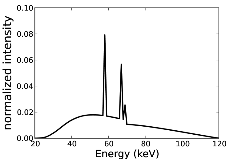
We demonstrate use of the one-step spectral CT algorithm on simulated transmission data modeling an ideal photon-counting detector. The X-ray spectrum, shown in Fig. 1, is assumed known. In modeling the ideal detector, the spectral response of an energy-windowed photon count measurement is taken to be the same as that of Fig. 1 between the bounding threshold energies of the window and zero outside. We conduct two studies. The first is focused on demonstrating convergence and application of the one-step algorithm with recovery of material maps for a two-material head phantom using the following minimization problems
and
The pseudo-code for TPL-TV and LSQ-TV is given explicitly in Appendix C. The second study simulates a more realistic study demonstrating application on an anthropomorphic chest phantom simulating multiple tissues/materials at multiple densities. For this study we demonstrate one-step image reconstruction of a mono-energetic image at energy using
Note that for monoenergetic image reconstruction, the TV constraint is placed on the monoenergetic image, but the optimization is performed over the individual material maps and the monoenergetic image is formed after the optimization using Eq. (11).
Aside from the system specification parameters, such as number of views, detector bins, and image dimensions, the algorithm parameters are the TV constraints for TPL-TV and LSQ-TV or for TPL-monoTV and the primal-dual step size ratio . The TV constraints or affect the image regularization, but is a tuning parameter which does not alter the solution of TPL-TV, LSQ-TV, or TPL-monoTV. It is used to optimize convergence speed of the one-step image reconstruction algorithm.
IV-A Head phantom studies with material map TV-constraints
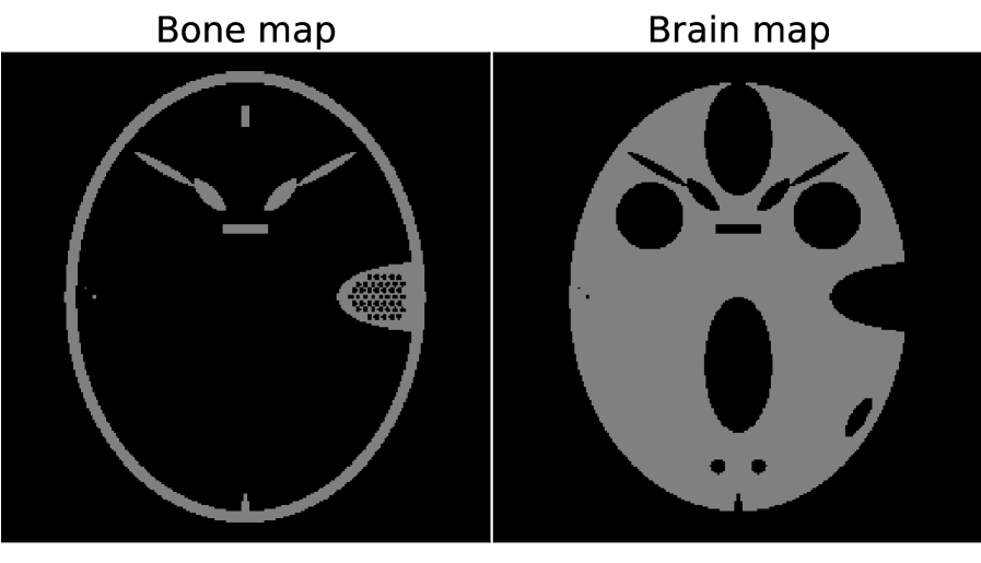
For the present studies, we employ a two-material phantom derived from the FORBILD head phantom shown in Fig. 2. The spectral CT transmission counts are computed by use of the discrete-to-discrete model in Eq. (4). The true material maps and are the 256256 pixel arrays shown in Fig. 2 and the corresponding linear X-ray coefficients and are obtained from the NIST tables available in Ref. [23] for energies ranging from 20 to 120 KeV in increments of 1 KeV. By employing the same data model as that used in the image reconstruction algorithm, we can investigate the convergence properties of the one-step algorithm.
For the head phantom simulations, the scanning configuration is 2D fan-beam CT with a source to iso-center distance of 50 cm and source to detector distance of 100 cm. The physical size of the phantom pixel array is cm2. The number of projection views over a full 2 scan is 128 and the number of detector bins along a linear detector array is 512. This configuration is undersampled by a factor of 4 [31]. Two X-ray energy windows are simulated with a spectral response for each window given by the spectrum shown in Fig. 1 in the energy ranges [20 KeV, 70 KeV] and [70 KeV, 120 KeV] for the first and second energy windows, respectively.
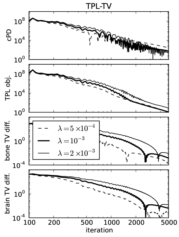
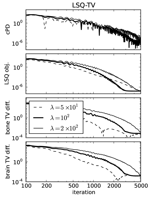
Ideal data study
For ideal, noiseless data several image metrics are plotted in Fig. 3 for different values of , and it is observed that the conditional primal-dual (cPD) gap and data discrepancy tend to zero while the material map TVs converge to the designed values. For this problem the convergence metrics are the cPD and material map TVs; the data discrepancy only tends to zero here due to the use of ideal data and in general when data inconsistency is present the minimum data discrepancy will be greater than zero. The convergence metrics demonstrate convergence of the one-step algorithm for the particular problem under study. It is important, however, to inspect these metrics for each application of the one-step algorithm, because there is no theoretical guarantee of convergence due to the re-expansion step in Eq. (60). From the present results it is clear that progress towards convergence depends on ; thus it is important to perform a search over .
TPL-TV LSQ-TV
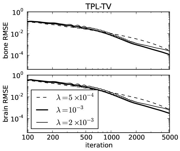
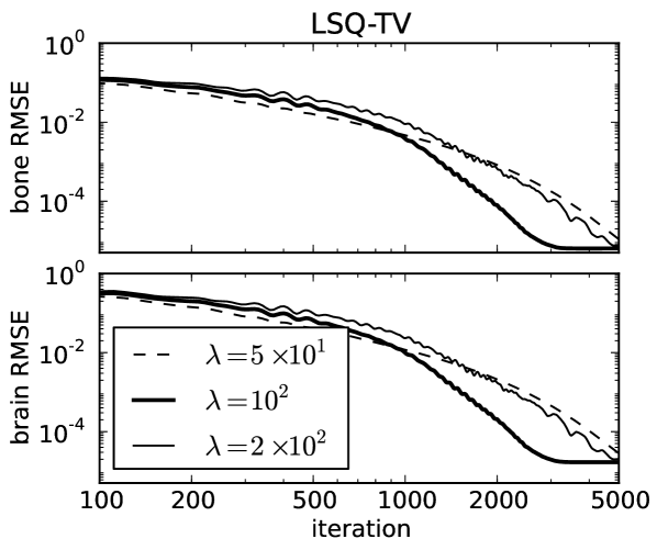
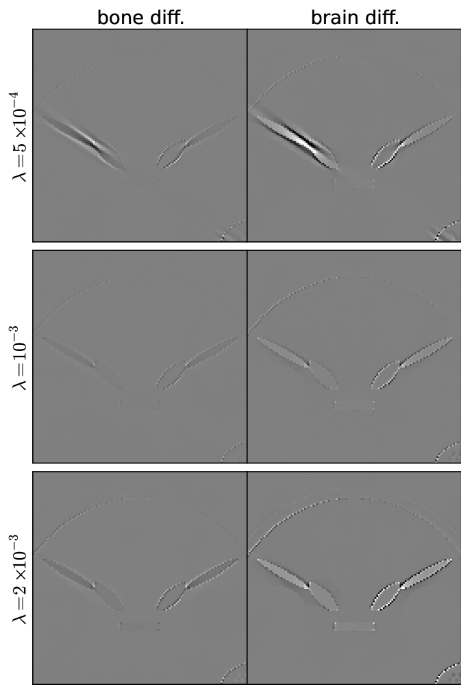
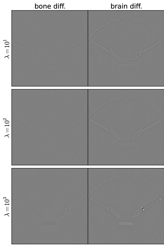
To demonstrate convergence of the material map estimates to the corresponding phantom, we plot image root-mean-square-error (RMSE) in Fig. 4 as a function of iteration number and show the map differences at the last iteration performed in Fig. 5. The material map estimates are seen to converge to the corresponding phantom maps despite the projection view-angle under-sampling. Thus we note that the material map TV constraints are effective at combatting these under-sampling artifacts just as they are for standard CT [32, 33]. The image RMSE curves only give a summary metric for material map convergence, and it is clear from the difference images displayed in narrow gray scale window that convergence can be spatially non-uniform. For these idealized examples the pre-conditioned one-step algorithm appears to be more effective for LSQ-TV than TPL-TV as the image RMSE attained for the former is significantly lower than that of the latter. In Fig. 4 curves for LSQ-TV at , the image RMSE curves plateau at due to the fact that the solution of LSQ-TV is achieved to the single precision accuracy of the computation.

Noisy data study
The noisy simulation parameters are identical to the previous noiseless study except that the spectral CT data are generated from the transmission Poisson model. The mean of the transmission measurements is arrived at by assuming total photons are incident at each detector pixel over the complete X-ray spectrum. As the simulated scan acquires only 128 views, the total X-ray exposure is equivalent to acquiring 512 views at photons per detector pixel.

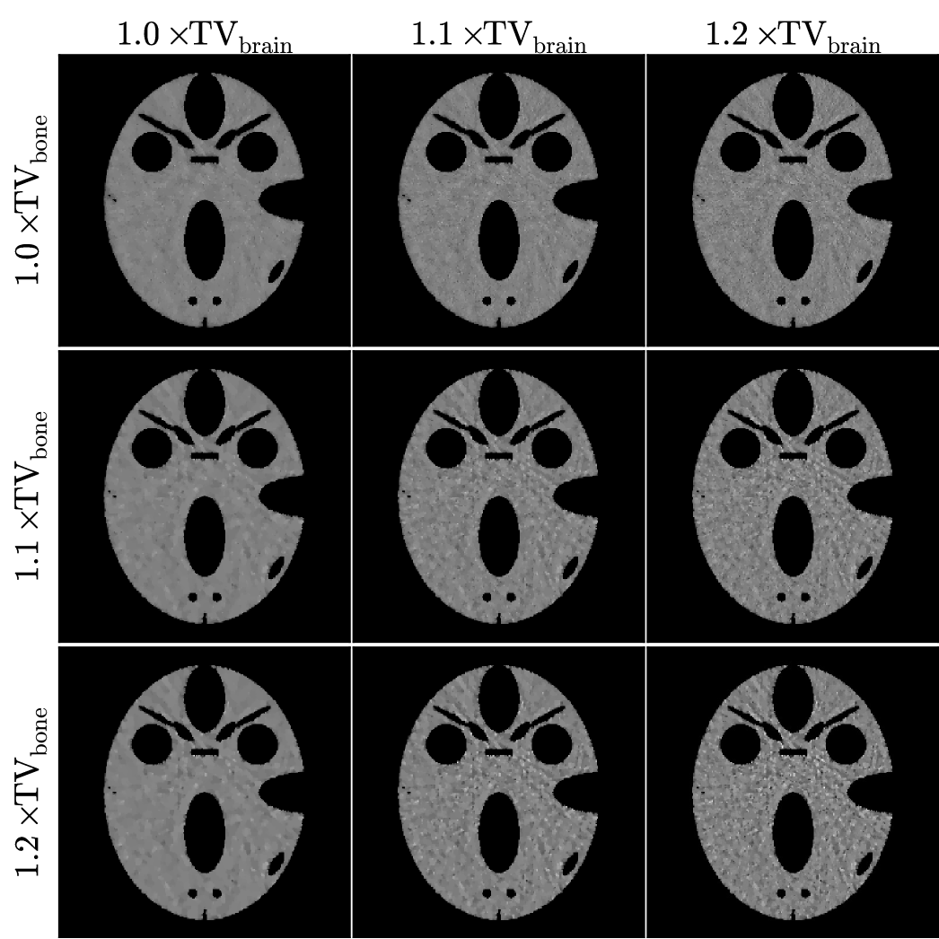
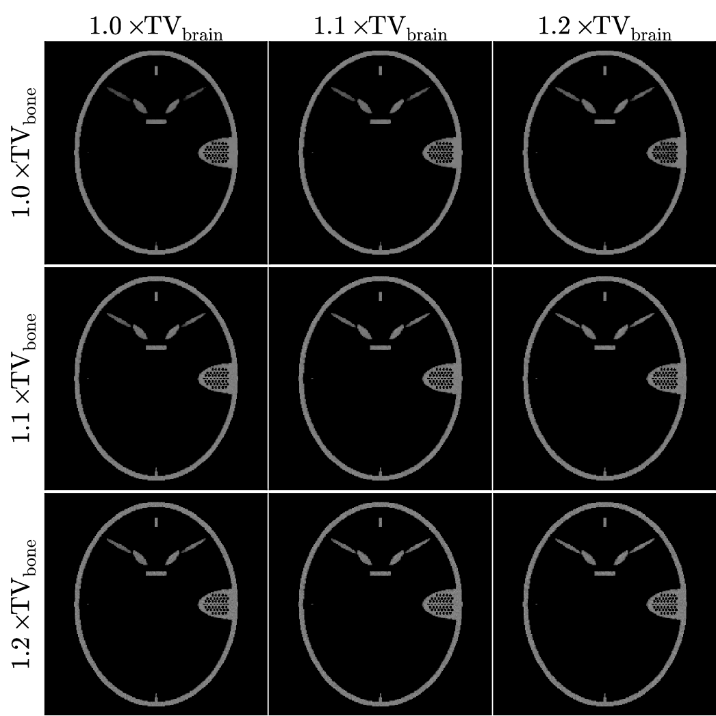
We obtain multiple material map reconstructions varying the TV constraints among values greater than or equal to the actual values of the known bone and brain maps. The results for TV-TPL are shown in Figs. 6 and 7, and those for TV-LSQ are shown in Figs. 8 and 9. In all images the bone and brain maps recover the main features of the true phantom maps, and the main difference in the images is the structure of the noise. The noise texture of the recovered brain maps appears to be patchy for lower TV and grainy for larger TV constraints. Also, in comparing the brain maps for TPL-TV in Fig. 7 and LSQ-TV in Fig. 9, streak artifacts are more apparent in the latter particularly for the larger TV constraint values.
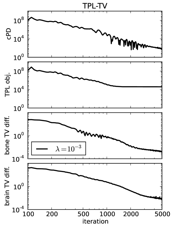
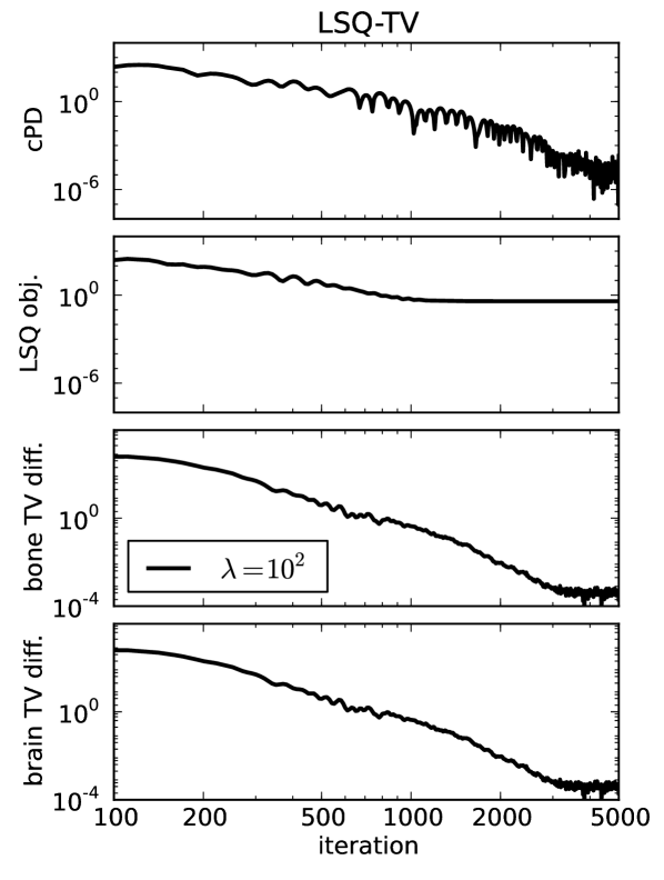
It is instructive to examine the convergence metrics in Fig. 10 and image convergence in Fig. 11 for this noisy simulation. The presentation parallels the noiseless results in Figs. 3 and 4, respectively. The differences are that results are shown for a single and the image RMSE is shown for two different TV-constraint settings in the present noisy simulations. The cPD and TV plots all indicate convergence to the solution for TPL-TV and LSQ-TV. Note, however, the value of the data discrepancy objective function settles on a positive value as expected for inconsistent data. The data discrepancy, however, does not provide a check on convergence. It is true that if the data discrepancy changes with iteration we do not have convergence, but the inverse is not necessarily true. It is also reassuring to observe that the convergence rates for the set values of are similar between the noiseless and noisy results. This similarity is also not affected by the fact that the TV constraints are set to different values in each of these simulations.
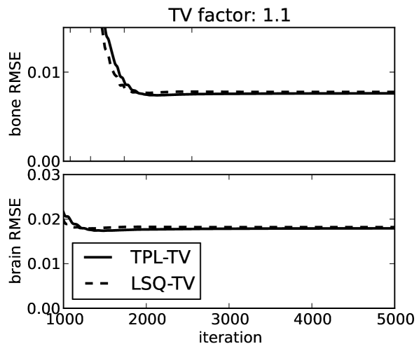
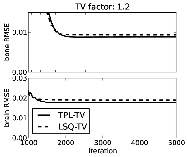
The RMSE comparison of the recovered material maps with the true phantom maps shown in Fig. 11 indicate an average error less than 1% for the bone map and just under 2% for the brain map (100 the RMSE values can be interpreted as a percent error because the material maps have a value of 0 or 1). The main purpose of showing these plots is to see quantitatively the difference between the TPL and LSQ data discrepancy terms. We would expect to see lower values of image RMSE for TPL-TV, because the simulated noise is generated by a transmission Poisson model. Indeed the image RMSE is lower for TPL-TV and the gap between TPL-TV and LSQ-TV is larger for looser TV constraints. We do point out that image RMSE may not translate into better image quality, because image quality depends on the imaging task for which the images are used. Task-based assessment would take into account features of the observed signal, noise texture, and possibly background texture and observer perception [34].
One of the benefits of using the TV constraints instead of TV penalties is that the material maps reconstructed using the TPL and LSQ data discrepancy terms can be compared meaningfully. The TV constraint parameters will result in material maps with exactly the chosen TVs, while to achieve the same with the penalization approach the penalty parameters must be searched to achieve equivalent TVs. Also generating simulation results becomes more efficient, because we can directly make use of the known phantom TV values.
IV-B Chest phantom studies with a mono-energetic image TV constraint
For the final set of results we employ an anthropomorphic chest phantom created from segmentation of an actual CT chest image. Different tissue types and densities are labeled in the image totaling 24 material/density combinations, including various soft tissues, calcified/bony regions, and Gadolinium contrast agent. To demonstrate the one-step algorithm on this more realistic phantom model, we select the TPL-monoTV optimization problem in Eq. (IV) for the material map reconstruction. The material basis is selected to be water, bone, and Gadolinium contrast agent. Using TPL-monoTV is simpler than TPL-TV in that only the energy for the mono-energetic image and a single TV constraint parameter is needed instead of three parameters – the TV for each of the material maps. There are potential advantages to constraining the TV of the material maps individually, but the purpose here is to demonstrate use of the one-step algorithm and accordingly we select the simpler optimization problem.
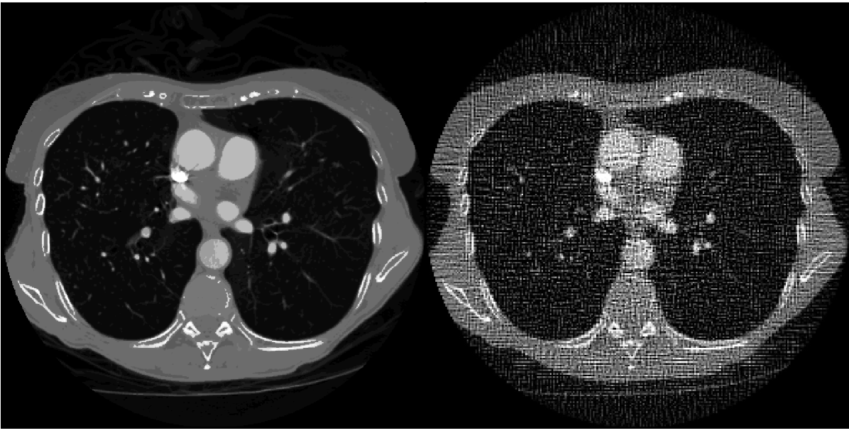
For the chest phantom simulations, the scanning configuration is again 2D fan-beam CT with a source to iso-center distance of 80 cm and source to detector distance of 160 cm. The physical size of the phantom pixel array is cm2. The number of projection views is 128 over a 2 scan. Five X-ray energy windows are simulated in the energy ranges [20 , 50], [50, 60], [60,80], [80,100], and [100, 120] keV. The lowest energy window is selected wider than the other four to avoid photon starvation. Noise is added in the same way as the previous simulation. The transmitted counts data follow a Poisson model with a total of photons per detector pixel. The monoenergetic image at 70 keV along with unregularized image reconstruction by TPL are shown in Fig. 12. The TPL mono-energetic image reconstruction demonstrates the impact of the simulated noise on the reconstructed image.
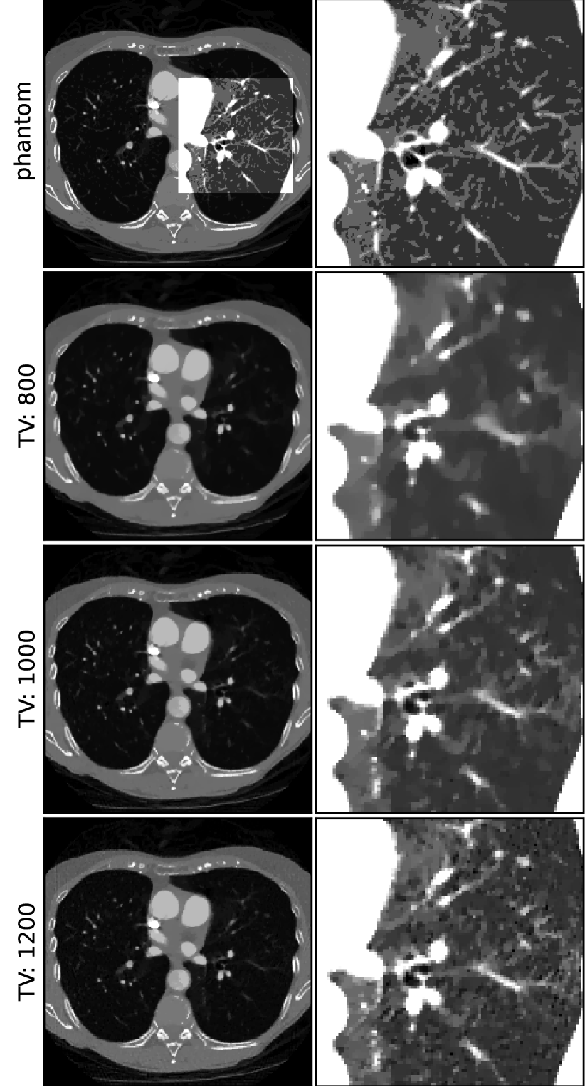
In Fig. 13 we show the resulting monoenergetic images from TPL-monoTV at three values of the TV constraint. The reconstructed images are shown globally in a wide gray scale and in an ROI focused on the right lung in a narrow gray scale window. The values of the TV constraint are selected based on visualization of the fine structures in the lung. For viewing these features, relatively low values of TV are selected. We note that in the global images the same TV values show the high-contrast structures with few artifacts. We point out that the one-step algorithm yields three basis material maps (not shown) and the mono-energetic images are formed by use of Eq. (11).
The selected optimization problems and simulation parameters are chosen to demonstrate possible applications of the one-step algorithm for spectral CT. Comparison of the TPL and LSQ data discrepancy in Figs. 7 and 9 does show fewer artifacts for TPL-TV, where the simulated noise model matches the TPL likelihood. In practice, we may not see the same relative performance on real data – the simulations ignore some important physical factors of spectral CT, and image quality evaluation depends on the task for which the images are used.
V Conclusion
We have developed a constrained one-step algorithm for inverting spectral CT transmission data directly to basis material maps. The algorithm addresses the associated non-convex data discrepancy terms by employing a local convex quadratic upper bound to derive the descent step. While we have derived the algorithm for TPL and LSQ data discrepancy terms, the same strategy can be applied to derive the one-step algorithm for other data fidelities. The one-step algorithm derives from the convex-concave optimization algorithm, MOCCA, which we have developed for addressing an intermediate problem arising from use of the local convex quadratic approximation. The simulations demonstrate the one-step algorithm for TV-constrained data discrepancy minimization, where the TV constraints can be applied to the individual basis maps or to an estimated monochromatic X-ray attenuation map.
Future work will investigate robustness of the one-step algorithm to data inconsistency due to spectral miscalibration error, X-ray scatter, and various physical processes involved in photon-counting detection. The one-step algorithm’s ability to incorporate basis map constraints in the inversion process should provide a means to control artifacts due to such inconsistencies. We are also pursuing a generalization to the present algorithm to allow for auto-calibration of the spectral response of the CT system.
Acknowledgements
This work was supported by NIH Grants R21EB015094, CA158446, CA182264, and EB018102. The contents of this article are solely the responsibility of the authors and do not necessarily represent the official views of the National Institutes of Health.
Appendix A Gradient of
Appendix B Positive semidefiniteness of and
Recall Eq. (18),
For ease of presentation, we collapse the double indices of
We show that
| (74) |
This inequality can be used to prove that the Hessians in Eqs. (21), (22), (23), and (24) are positive semidefinite by setting equal to , , , and , respectively.
To prove Eq. (74), we expand in unit vectors
and show for any vector that
| (75) |
Fixing , we define the vector with components or using the unit vector
From the definition of , we note that for all and . By the definition of , the left-hand side of Eq. (75), lhs, is
| lhs | |||
and by the Cauchy-Schwartz inequality,
| lhs | |||
This proves the inequality in Eq. (75).
Appendix C Derivation of one-step algorithm for TPL-TV and LSQ-TV with -preconditioning
TV-constrained optimization
To derive the one-step algorithm used in the Results section, we write down the intermediate convex optimization problem that involves the first block of the local quadratic upper bound to or
| (77) |
That only the first block of the full quadratic expression is explained in Sec. III-B4 and the form of , and given in Sec. III-B2 determines whether we are addressing TPL-TV or LSQ-TV . The data discrepancy term of this optimization problem is the same as the objective function of Eq. (58), but it differs from Eq. (58) in that we have added the convex constraints on the material map TV values. We write Eq. (77) using indicator functions (see Eq. (6)) to code the TV constraints and we introduce the -preconditioning transformation described in Sec. III-C
| (78) |
where are the transformed (-preconditioned) material maps from Sec. III-C. Note that the TV constraints apply to the untransformed material maps .
Writing constrained TV optimization in the general form
To derive the CP primal-dual algorithm, we write Eq. (78) in the form of Eq. (26). We note that all the terms involve a linear transform of , and accordingly we make the following assignments
where
Note that we use the short-hand that the gradient operator, , applies to each of the material maps in the composite material map vector, . The Legendre transform in Eq. (28) provides the necessary dual functions , , and . By direct computation
| (79) |
From Sec. 3.1 of Ref. [27]
| (80) |
Convex conjugate of
We sketch the derivation of , and for this derivation we drop the “grad” subscript.
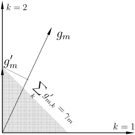
The Legendre transform maximization over the variable , dual to the material map gradients, is reduced to a maximization over the spatial magnitude because the indicator function is independent of the spatial direction of and the term is maximized when the spatial direction of line up with ; hence the term is replaced by , which we explicitly write as a sum over the material index . The maximization and summation order can be switched, because each of the terms in the summation are independent of each other. Evaluation of the maximization over can be seen in the diagram shown in Fig. 14. Accordingly we find
| (81) |
Dual maximization of Eq. (78)
The material map TV proximity step
In order to derive the TPL-TV and LSQ-TV one step algorithms, we need to derive the proximity minimization in Eq. (54)
The proximity problem splits into “sino” and “grad” sub-problems and the “sino” sub-problem results in Eq. (63). We solve here the “grad” proximity optimization to obtain the pseudo-code for TPL-TV and LSQ-TV
Dropping the “grad” subscript on , we employ the Moreau identity which relates the proximity optimizations between a function and its dual
| (83) |
The dual “grad” update separates into the individual material map components
To simplify the proximity minimization we set
The proximity minimization is a projection of onto a weighted -ball.
If is inside the weighted -ball, i.e. , the function returns . If is outside the weighted -ball, i.e. , there exists an such that
The parameter is defined implicitly
and it can be determined by any standard root finding technique applied to
where the search interval is .
The pseudocode for TPL-TV and LSQ-TV
Having derived the TV constraint proximity step, we are in a position to write the complete pseudocode for the one-step algorithm including the TV constraints. We do employ the -preconditioning that orthogonalizes the linear attenuation coefficients, but we drop the prime notation on and .
| (88) | ||||
| (93) | ||||
The final material maps after iterations are obtained by applying the inverse preconditioner
For all the results presented in the article, all variables are initialized to zero.
References
- [1] K. Taguchi and J. S. Iwanczyk, “Vision 20/20: Single photon counting x-ray detectors in medical imaging,” Med. Phys., vol. 40, p. 100901, 2013.
- [2] R. E. Alvarez and A. Macovski, “Energy-selective reconstructions in X-ray computerised tomography,” Phys. Med. Biol., vol. 21, pp. 733–744, 1976.
- [3] P. M. Shikhaliev, “Energy-resolved computed tomography: first experimental results,” Phys. Med. Biol., vol. 53, pp. 5595–5613, 2008.
- [4] T. G. Schmidt, “Optimal “image-based” weighting for energy-resolved CT,” Med. Phys., vol. 36, pp. 3018–3027, 2009.
- [5] A. M. Alessio and L. R. MacDonald, “Quantitative material characterization from multi-energy photon counting CT,” Med. Phys., vol. 40, p. 031108, 2013.
- [6] E. Roessl and R. Proksa, “K-edge imaging in x-ray computed tomography using multi-bin photon counting detectors,” Phys. Med. Biol., vol. 52, pp. 4679–4696, 2007.
- [7] J.-P. Schlomka, E. Roessl, R. Dorscheid, S. Dill, G. Martens, T. Istel, C. Bäumer, C. Herrmann, R. Steadman, G. Zeitler, A. Livne, and R. Proksa, “Experimental feasibility of multi-energy photon-counting K-edge imaging in pre-clinical computed tomography,” Phys. Med. Biol., vol. 53, pp. 4031–4047, 2008.
- [8] E. Roessl, D. Cormode, B. Brendel, K.-J. Engel, G. Martens, A. Thran, Z. Fayad, and R. Proksa, “Preclinical spectral computed tomography of gold nano-particles,” Nucl. Inst. Meth. A, vol. 648, pp. S259–S264, 2011.
- [9] D. P. Cormode, E. Roessl, A. Thran, T. Skajaa, R. E. Gordon, J.-P. Schlomka, V. Fuster, E. A. Fisher, W. J. M. Mulder, R. Proksa, and Z. A. Fayad, “Atherosclerotic plaque composition: Analysis with multicolor CT and targeted Gold nanoparticles,” Radiology, vol. 256, pp. 774–782, 2010.
- [10] E. Roessl, B. Brendel, K.-J. Engel, J.-P. Schlomka, A. Thran, and R. Proksa, “Sensitivity of photon-counting based K-edge imaging in X-ray computed tomography.” IEEE Trans. Med. Imaging, vol. 30, pp. 1678–1690, 2011.
- [11] C. O. Schirra, E. Roessl, T. Koehler, B. Brendal, A. Thran, D. Pan, M. A. Anastasio, and R. Proksa, “Statistical reconstruction of material decomposed data in spectral CT,” IEEE Trans. Med. Imaging, vol. 32, pp. 1249–1257, 2013.
- [12] G. N. Hounsfield, “Computerized transverse axial scanning (tomography): Part 1. Description of system,” Brit. J. Radiol., vol. 46, pp. 1016–1022, 1973.
- [13] C. Maaß, M. Baer, and M. Kachelrieß, “Image-based dual energy CT using optimized precorrection functions: A practical new approach of material decomposition in image domain,” Med. Phys., vol. 36, pp. 3818–3829, 2009.
- [14] R. A. Brooks, “A quantitative theory of the Hounsfield unit and its application to dual energy scanning.” J. Comp. Assist. Tomography, vol. 1, pp. 487–493, 1977.
- [15] J. A. Fessler, I. A. Elbakri, P. Sukovic, and N. H. Clinthorne, “Maximum-likelihood dual-energy tomographic image reconstruction,” vol. 4684, 2002, pp. 38–49.
- [16] I. A. Elbakri and J. A. Fessler, “Statistical image reconstruction for polyenergetic X-ray computed tomography,” IEEE Trans. Med. Imaging, vol. 21, pp. 89–99, 2002.
- [17] J. Chung, J. G. Nagy, and I. Sechopoulos, “Numerical algorithms for polyenergetic digital breast tomosynthesis reconstruction,” SIAM J. Imaging Sci., vol. 3, no. 1, pp. 133–152, 2010.
- [18] C. Cai, T. Rodet, S. Legoupil, and A. Mohammad-Djafari, “A full-spectral Bayesian reconstruction approach based on the material decomposition model applied in dual-energy computed tomography,” Med. Phys., vol. 40, p. 111916, 2013.
- [19] Z. Ruoqiao, J.-B. Thibault, C.-A. Bouman, K. D. Sauer., and J. Hsieh, “Model-based iterative reconstruction for dual-energy X-ray CT using a joint quadratic likelihood model,” IEEE Trans. Med. Imaging, vol. 33, pp. 117–134, 2014.
- [20] Y. Long and J. A. Fessler, “Multi-material decomposition using statistical image reconstruction for spectral CT,” IEEE Trans. Med. Imaging, vol. 33, pp. 1614–1626, 2014.
- [21] A. Sawatsky, Q. Xu, C. O. Schirra, and M. A. Anastasio, “Proximal admm for multi-channel image reconstruction in spectral X-ray CT,” IEEE Trans. Med. Imaging, vol. 33, pp. 1657–1668, 2014.
- [22] K. Nakada, K. Taguchi, G. S. K. Fung, and K. Armaya, “Joint estimation of tissue types and linear attenuation coefficients for photon counting CT,” Med. Phys., vol. 42, pp. 5329–5341, 2015.
- [23] J. H. Hubbell and S. M. Seltzer, “Tables of x-ray mass attenuation coefficients and mass energy-absorption coefficients 1 keV to 20 MeV for elements Z= 1 to 92 and 48 additional substances of dosimetric interest,” National Inst. of Standards and Technology-PL, Gaithersburg, MD (United States). Ionizing Radiation Div., Tech. Rep., 1995.
- [24] D. S. Rigie and P. J. L. Rivière, “Joint reconstruction of multi-channel, spectral CT data via constrained total nuclear variation minimization,” Phys. Med. Biol., vol. 60, pp. 1741–1762, 2015.
- [25] A. Chambolle and T. Pock, “A first-order primal-dual algorithm for convex problems with applications to imaging,” J. Math. Imag. Vis., vol. 40, pp. 120–145, 2011.
- [26] T. Pock and A. Chambolle, “Diagonal preconditioning for first order primal-dual algorithms in convex optimization,” in International Conference on Computer Vision (ICCV 2011). Barcelona, Spain: IEEE, 2011, pp. 1762–1769.
- [27] E. Y. Sidky, J. H. Jørgensen, and X. Pan, “Convex optimization problem prototyping for image reconstruction in computed tomography with the Chambolle-Pock algorithm,” Phys. Med. Biol., vol. 57, pp. 3065–3091, 2012.
- [28] E. Y. Sidky, R. Chartrand, J. M. Boone, and X. Pan, “Constrained TV minimization for enhanced exploitation of gradient sparsity: Application to CT image reconstruction,” J. Trans. Engineer. Health Med., vol. 2, p. 1800418, 2014.
- [29] J. S. Jørgensen and E. Y. Sidky, “How little data is enough? Phase-diagram analysis of sparsity-regularized X-ray CT,” Phil. Trans. Royal Soc. A, vol. 373, p. 20140387, 2015.
- [30] R. F. Barber and E. Y. Sidky, “MOCCA: mirrored convex/concave optimization for nonconvex composite functions,” 2015, http://arxiv.org/abs/1510.08842.
- [31] J. S. Jørgensen, E. Y. Sidky, and X. Pan, “Quantifying admissible undersampling for sparsity-exploiting iterative image reconstruction in X-ray CT,” IEEE Trans. Med. Imaging, vol. 32, pp. 460–473, 2013.
- [32] E. Y. Sidky, C.-M. Kao, and X. Pan, “Accurate image reconstruction from few-views and limited-angle data in divergent-beam CT,” J. X-ray Sci. Tech., vol. 14, pp. 119–139, 2006.
- [33] E. Y. Sidky and X. Pan, “Image reconstruction in circular cone-beam computed tomography by constrained, total-variation minimization,” Phys. Med. Biol., vol. 53, pp. 4777–4807, 2008.
- [34] H. H. Barrett and K. J. Myers, Foundations of Image Science. Hoboken, NJ: John Wiley & Sons, 2004.