An Algorithm for the Continuous Morlet Wavelet Transform

Richard Büssow Institute of Fluid Mechanics and Engineering Acoustics, Berlin University of Technology, Einsteinufer 25, 10587 Berlin richard.buessow@tu-berlin.de

Abstract

This article consists of a brief discussion of the energy density over time or frequency that is obtained with the wavelet transform. Also an efficient algorithm is suggested to calculate the continuous transform with the Morlet wavelet.
The energy values of the Wavelet transform are compared with the power spectrum of the Fourier transform. Useful definitions for power spectra are given.
The focus of the work is on simple measures to evaluate the transform with the Morlet wavelet in an efficient way. The use of the transform and the defined values is shown in some examples.

keywords:

morlet power spectrum , time domain , impulse response , dispersion

PACS:

43.60 Hj

1 Introduction

The wavelet transform is a method for time-frequency analysis. The application for acoustic signals can be found in several publications. These publications deal for example with the analysis of dispersive waves [1, 2], source or damage localization [3, 4], investigation of system parameters [5, 6] or active control [7]. A comparison of the short time Fourier transform and the wavelet transform is done by Kim et.al. [8]. It is found that the continuous wavelet transform CWT of acoustic signals is a promising method to obtain the time - frequency energy distribution of a signal.
Another sort are wavelets for spatial transforms, that are an effective tool for damage localisation[9, 10].
The aim of this publication is to present an algorithm for the continuous wavelet transform CWT with the Morlet wavelet. Caprioli et al. state in [11] that ”The high computational complexity (of the CWT) is not a serious worry for today’s computer power; still it might be an obstacle for an ”on line” application.” Alternatives to the CWT are characterised by low computational complexity, but the best results are obtained by the CWT. The presented algorithm implements simple measures to reduce the computational complexity of the CWT. An implementation in Java is written and is open source and freely available online¹¹1http://www.tu-berlin.de/fb6/ita.
Nevertheless it should be mentioned that the Wigner approximation is also very useful in the given context. A recent publication is for example [12]. Other methods, that are adapted to the analysis of dispersive waves are discussed in [13, 14].
This publication starts with a discussion of the energy values that are obtained by the wavelet transform. It follows a description of an efficient algorithm to evaluate the transform.

2 Morlet Wavelet Transform

The theoretical background of the wavelet transform can be found in textbooks [15, 16]. Only the used definitions are stated. The wavelet transform with the wavelet $\psi$ of a signal $y(t)$ is defined as

W_{\psi}^{y}(a,b)=\frac{1}{\sqrt{c_{\psi}|a|}}\int\limits_{-\infty}^{\infty}y(t)\psi\left(\frac{t-b}{a}\right)\>dt,

(1)

where $a$ is called dilatation and $b$ translation parameter. The Morlet wavelet $\psi$ which is sometimes called Gabor wavelet is given by

\psi(t)=e^{-\beta\frac{t^{2}}{2}}e^{j\omega_{0}t}

(2)

and $c_{\psi}=\sqrt{\pi/\beta}$ . The values $\beta=\omega_{0}^{2}$ and $\omega_{0}$ are defined in a particular application so that the admissibility condition is valid [16]. The function (2) is called mother wavelet.
The Morlet wavelet is common for the time frequency analysis of acoustic signals. For a comparison of different so called mother wavelets see Schukin et. al. [17].

2.1 Comparing Fourier and wavelet transform

When using the Fourier transform one usually develops the spectrogram. The wavelet transform has scaling factors. The analog to the spectrogram is the scalogram defined as

|W_{\psi}^{y}(a,b)|^{2}.

(3)

The scalogram is a measure of the energy distribution over time shift $b$ and scaling factor $a$ of the signal. It holds that the energy $E_{y}$ of a signal $y$ is

E_{y}=\int\limits_{-\infty}^{\infty}|y(t)|^{2}\>dt=\int\limits_{-\infty}^{\infty}\int\limits_{-\infty}^{\infty}|W_{\psi}^{y}(a,b)|^{2}\frac{da\>db}{a^{2}}.

(4)

If instead of the scaling factor $a$ the frequency value $f=1/a$ is used, the value $f$ is only the real frequency if $\omega_{0}=2\pi$ .
It follows with $da=\frac{da}{df}\>df=-\frac{1}{f^{2}}\>df$ that

E_{y}=\int\limits_{-\infty}^{\infty}\int\limits_{-\infty}^{\infty}|W_{\psi}^{y}(f,b)|^{2}\>df\>db.

(5)

It is possible to divide this total energy into an energy density over time and over frequency. This is achieved by one integration over frequency or time. The energy density over time is defined by

E_{t}(b)=\int\limits_{-\infty}^{\infty}|W_{\psi}^{y}(f,b)|^{2}\>df.

(6)

The energy density over frequency, or the energy density spectrum is defined by

E_{f}(f)=\int\limits_{-\infty}^{\infty}|W_{\psi}^{y}(f,b)|^{2}\>db.

(7)

2.1.1 Power signals

The value $|W_{\psi}^{y}(f,b)|^{2}$ is sometimes called Morlet power spectrum, but here the term energy density is used. A Comparision of the values obtained with the Fourier transform and the wavelet transform is, for example, given in [18]. A power signal is characterized by

P=\frac{1}{T}\int\limits_{-\infty}^{\infty}|x(t)|^{2}\>dt<\infty.

(8)

If the wavelet transform is applied to a power signal one recognises that for higher frequencies the energy density is lower, as shown in the examples in section 4. To achieve a better match, Shyu [19] proposes a modified equal amplitude wavelet power spectrum that is given by

\mbox{MPS}=\frac{f}{c_{\psi}}\>|W_{\psi}^{y}(f,b)|^{2}.

(9)

The above definition corresponds more closely to power spectra obtained with the discrete Fourier transform. This can be explained since $P=\frac{1}{T}E$ and $c_{\psi}a$ is the effective length of the wavelet so $T_{eff}=c_{\psi}/f$ is the value to scale the energy density. Since one is usually familiar with power spectra, the above definition (9) is useful but a problem is that

P\neq\int\limits_{-\infty}^{\infty}\int\limits_{-\infty}^{\infty}\mbox{MPS}\>df\>db.

(10)

This fact can be compared with the windowed Fourier transformation. If the window like for example, the flat top is defined so that the peak value is constant²²2Which is strictly true only if $f_{n}=T/(2n\pi)$ , but the window should minimize the deviation., it follows that the effective noise band width is altered by the windowing function. The Morlet wavelet transform can be interpreted as a windowed Fourier transformation with a frequency dependent window size.

Alternative definition of the power spectrum

In the following a new definition of the power spectrum is given. It is defined analogous to the discrete Fourier transform, so that the power can be calculated by summation of the power values. The discrete Fourier transform is a filter with the bandwidth $\Delta f$ , so each value of the power spectrum is the integral over $\Delta f$ . The power spectrum that is defined with the energy values of the discrete continuous Morlet wavelet transform is

P_{i}=\frac{\Delta f_{i}}{T}E_{f}(f_{i}).

(11)

Given the shape of the Morlet wavelet, the only sensible scaling of the frequency values is logarithmic. With this prerequisite the values $P_{i}$ follow the same tendency as equation (9). Using equation (11) the total power is given by $P=\sum_{i}P_{i}$ .
From equation (11) and $\Delta t=T/N_{t}$ , where $N_{t}$ is the number of time values, it follows that

P_{d}(i,j)=\frac{1}{T}\,\Delta f_{i}\,\Delta t\,|W_{\psi}^{y}(f_{i},b_{j})|^{2}=\frac{\Delta f_{i}}{N_{t}}|W_{\psi}^{y}(f_{i},b_{j})|^{2}

(12)

is a reasonable definition for the power spectrum over time. An example for a power signal is given in section 4.1.

2.1.2 Energy signals

However, the discrete Fourier Transform is usually the best method to work with power signals. The wavelet transform in contrast is suited to work with energy signals, for which

E=\int\limits_{-\infty}^{\infty}|x(t)|^{2}\>dt<\infty

(13)

is true. It is useful to use the value $E_{f}$ for comparing Fourier and Wavelet spectra in this case. This is done by calculating

E_{f}(i)=P_{i}\frac{T}{\Delta f_{i}}

(14)

from the power spectrum obtained with the Fourier transform. An example of an energy signal is given in 4.2.

3 CWT Algorithm

Usually the continuous wavelet transform is implemented in a direct algorithm. The starting point is a program written by Hayashi [20], where the integral in equation (1) is implemented by a simple summation over the elements. Typical values for the scaling parameter $a$ are 20 to 40, where $a_{n}=\alpha^{n}$ , with $\alpha=\sqrt[4]{2}$ . The time shift parameter is $b_{m}=m\Delta t$ , where $0\leq m\leq N$ .
The algorithm to calculate the wavelet transform of a discrete signal $y_{i}$ of the length $N$ is for each $a_{n}$ :

1.

Calculate $\psi_{i}$ , of the length $2N$ , $b_{m}=m\Delta t$ with $\omega_{0}=\sqrt{2}\pi/\Delta t$ .
2.

Shift $\psi$ about $m$ : $\sum_{i}^{N}y_{i}\cdot\psi_{N-m+i}$

The frequency is given by $f=\frac{\omega_{0}}{2\pi a_{n}}$ .

3.1 Improved algorithm

The continuous wavelet transform is very inefficient compared with the discrete wavelet transform. A brief description of a new algorithm follows which introduces ideas that are crucial for the high efficiency of the discrete wavelet transform DWT. Besides the following improvements the program calculates the corresponding frequency values and energy or power distributions that are defined in section 2.1.

3.1.1 Effective Compact support

The outer parts of the wavelet $|t|\gg 0$ have no significant contribution to the result because of the exponentially decaying envelope term $e^{-\beta t^{2}/2}$ which acts like a window, known as the windowed Fourier transform. Due to the limited floating point precision of a computer, the outer parts will not contribute to the integral in equation (1).
An a-priori estimation of the effective wavelet length is made here. For $t=0$ the envelope has its maximum which is unity. The length is chosen so, that for all $|t|>|t_{max}|$ the envelope is smaller than the precision. For a 64 bit floating point number this means that

	$\displaystyle e^{-\beta t_{max}^{2}/2}$	$\displaystyle=$	$\displaystyle 2.22\cdot 10^{-16}$
	$\displaystyle\|t_{max}\|$	$\displaystyle=$	$\displaystyle 8.49/\sqrt{\beta}.$		(15)

Strictly the outer parts can still contribute to the integral (1) especially if $y$ is a transient function, but in practise even a weaker definition does not show a significant effect.
The concept of neglecting the outer parts is called effective compact support. Note that to develop the transform the wavelet is scaled with $t/a$ . A general straight forward implementation is not possible, due to the discrete time values. This is a reason why the discrete wavelet transform uses scaling values that are defined by $a_{n}=2^{n}$ , where $n$ is an integer value.
The actual implementation works in the following way. The length of the wavelet that represents the lowest frequency $f_{min}$ is chosen so that $T/\Delta t=2^{N}$ . The mixed approach is that the wavelet length is halved for each doubling of the frequency, so for each value $f_{n}=2^{n}f_{min}$ , and left otherwise unchanged. For all frequency values $f_{i}$ for which $f_{n}=2^{n}f_{min}<f_{i}<2^{n+1}f_{min}=f_{n+1}$ holds, it follows that the support of the wavelet is even longer than $t_{max}$ . The reason for this effect is that also $t_{max}$ is scaled and so for a constant length and a higher frequency the support of the mother wavelet is longer.

3.1.2 Frequency dependent time shift

Due to the argument $\frac{t-b}{a}$ of the wavelet $\psi$ in (1) the transform can be interpreted as a convolution of a signal $y$ and a wavelet $\psi$

y\ast\psi=\int\limits_{-\infty}^{\infty}y(t)\psi(t-\tau)\>dt.

(16)

With the scaled argument $t/a$ and $\tau=b/a$ equation (1) follows. The algorithm that is outlined in section 3 does actually not set the translation parameter $b$ , but $b/a$ . It is the highest precision of the continuous translation parameter $b$ with discrete time values. But it is inefficient, since the whole wavelet and its time resolution are scaled with $a$ . The resolution depends on the wavelength. If one increases the time shift for lower frequencies this does not result in a less accurate resolution. Like for the effective compact support the translation parameter is adjusted for each doubling of the frequency.
The implementation uses the frequency dependent length of the a period $T_{\lambda}=1/f$ . The time shift parameter $b$ is defined relative to the period length $T_{\lambda}$ and an arbitrary dyadic factor $2^{n_{b}}$ in a way that $T_{\lambda}/2^{n_{b}}\geq b>T_{\lambda}/2^{n_{b}+1}$ is valid. The details can be found in the Java-code.
In some cases the values given above are not fully applicable. For example for frequencies $f>f_{s}/2^{n_{b}}$ , with the sampling frequency $f_{s}$ , the smallest possible shift is $\Delta t$ which can be bigger than $T_{\lambda}/2^{n_{b}}$ , but it is the highest possible precision. The default value is $2^{n_{b}}=16$ , which results in a high resolution where a difference to a higher resolution is not recognizable. With this measure a reduced computational effort is achieved.
Together with the compact support it is possible to use an amount of 200 scaling factors instead of 20 and wait a few seconds for the transform to be calculated.

3.1.3 Frequency dependent truncated boundaries

One may interpret $y(t)$ as an infinite signal of which a part of the length $T$ is known. The convolution of the wavelet over the signal results in a considerable violation of the admissibility condition since all the parts of the wavelet that lie outside the known signal must vanish. In practise this results in invalid data at the boundaries. When working with the compact support this is avoided if the algorithm guaranties that the whole wavelets always fits in the signal. Since the compact support of the wavelet will be shorter for high frequencies this results in a frequency dependent truncation. This measure is also implemented in [21].

3.2 Fast Morlet wavelet transform

A fast implementation is described in [21] and often called fast Morlet wavelet transform. The convolution in equation (1) is implemented by building the DFT of the wavelet and the analysed function, multiplying them and building the inverse Fourier transform. Since the DFT is calculated with the fast Fourier transform (FFT) algorithm, the computational effort is greatly reduced compared with [20].

3.3 Computational effort

This section will compare the order of the amount of operations that are needed for each implementation. Since the amount of operations depends on the actual implementation such an investigation is beyond the scope of this investigation.

AGU-implementation: For the implementation [20] the signal of length $N$ has to be multiplied $N$ times with the wavelet. For $M$ scaling factors the order of the amount of operations is $O(M\times N^{2})$ .
Fast Morlet Wavelet transform: The FFT has a computational effort of $O(log(N)N)$ , if $N$ is a power of two. It follows that the order of operation for the fast Morlet wavelet transform is $O(M\times log(N)N)$ .
New algorithm: According to section 3.1.1 the number of points of the wavelet $N_{w}$ is independent of the signal length $N$ . For a given frequency value $f_{i}$ the number of points is inversely dependent on the frequency $N_{w}\sim 1/f_{i}$ .
According to section 3.1.2 the translations parameter is also inversely dependent on the frequency $b_{i}\sim 1/f_{i}$ . The wavelet has to be multiplied $N/b_{i}$ times with the signal. Since $N_{w}<N$ the amount of multiplications is $N_{w}N/b_{i}$ . It follows that the order of the amount of multiplications for a given frequency value is $O(N)$ . The resulting overall effort is $O(M\times N)$ .

3.3.1 Benchmark

The consumed time for the transform depends on many other factors. It is only an indication for the amount of operation that actually have to be performed. Important factors that effect the computation time is the systems memory and the implementation itself.
The benchmark compares the standard Morlet wavelet transform (st), the fast Morlet wavelet transform (fast) and the described new Algorithm (new) in a typical application.
The standard Morlet wavelet transform is implemented with Matlab’s conv() function, that implements the convolution with a Matlab’s filter() function. Matlab’s profiler shows that $99.3\%$ of the computational time is used by the function conv() which is optimized.
The fast Morlet wavelet transform is implemented by a self-written convolution function that uses Matlabs highly optimized fft() function. The fft()-function itself chooses the presumable best algorithm for the application. The FFT algorithm needs a number of points that are an integer power of two $2^{n}$ . This can be problematic if one wants to adjust the length of a window so that it fits the discrete best case frequencies $f_{n}=T/(2n\pi)$ . This defiancy does not apply to the continuous wavelet transform.
The described algorithm is implemented with Java and called from Matlab. It is not optimised and it is known that Java programs of this sort usually suffer a 50-fold performance degradation [22] compared to native Fortran or similar applications. The intention of the implementation is to follow the guidelines for software engineering: Build the functionality first and do the optimization afterwards. The advantages of Java are that it is platform independent, has an easy to use interface to Matlab and no special or commercial libraries are needed.

N	$2^{8}$	$2^{9}$	$2^{10}$	$2^{11}$	$2^{12}$	$2^{13}$	$2^{14}$	$2^{15}$	$2^{16}$	$2^{17}$
st in s	0.51	1.90	7.85	27.3	106	417	1602	6445
$\frac{T\times 10^{-6}}{N^{2}}$	0.79	0.72	0.75	0.65	0.63	0.63	0.60	0.60
fast in s	0.16	0.27	0.49	0.80	1.38	3.15	6.76	16.48
$\frac{T\times 10^{-3}}{N\log(N)}$	0.39	0.29	0.23	0.17	0.16	0.15	0.14	0.14
new in s	0.07	0.23	0.34	0.45	0.83	1.37	2.62	4.83	9.12	18.16
$\frac{T\times 10^{-3}}{N}$	0.27	0.45	0.33	0.22	0.20	0.17	0.16	0.15	0.14	0.14

Table 1: Computation time for three different algorithms: standard (st), fast and new Morlet wavelet transform and for different sizes.

Table 1 shows the computational time for the same $M=200$ frequency values and a maximum frequency $f_{max}=f_{s}/8$ . It is assumed that measurements are often taken with a portable computer, so a Samsung X20 notebook is chosen, equipped with Pentium M CPU at 1.73 GHz and 1GB main memory. The parameters for the new transform were chosen such that the results are identical, a time shift parameter of $T_{\lambda}/4$ and $t_{max}=5.6s$ . The results show a good repeatability and the same tendency on other computers.
The order of operations that is derived in section 3.3 is validated with the normalised computational time $T/N^{2}$ for the standard, $T/(N\log(N))$ for the fast and $T/N$ for the new algorithm. If the computational time would solely depend on the amount of operations the normalised computational time should be constant.
When using the standard and fast algorithms the size of the memory limited the test to a maximum number of $2^{15}$ points. With the new algorithm it was possible to calculate the transform also for $2^{18}$ and $2^{19}$ in a time of $37.25s$ and $69.16s$ . These values also indicate that the estimation of a linear increasing number of operations is valid, since $\frac{T\times 10^{-3}}{N}$ is again $0.14$ . For a typical sampling frequency of $f_{s}=48kHz$ this means that it is possible to analyse around $10s$ .

4 Examples

The capabilities of the wavelet transform and the described algorithm are demonstrated in the examples below.

4.1 Power signal

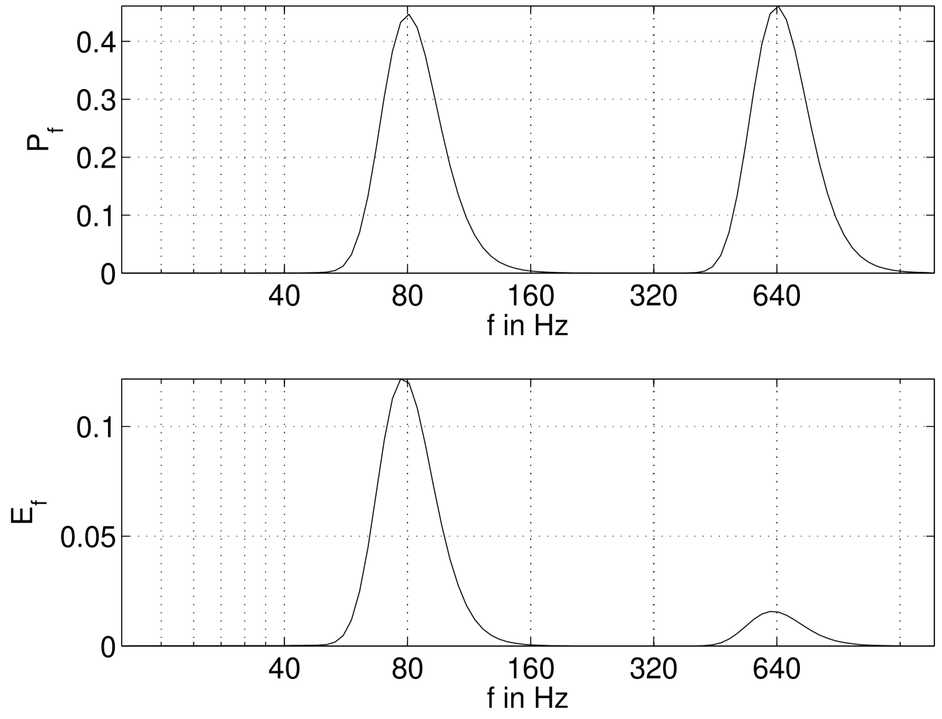
A typical power signal is the sine function. Consider the example with a changing frequency

y(t)=\left\{\begin{array}[]{l}A\sin(2\pi f_{1}t)\mbox{ for }t<1/2\\ A\sin(2\pi f_{2}t)\mbox{ for }t>1/2,\end{array}\right.

(17)

with $\Delta t=2^{-13}$ , $f_{1}=80Hz$ , $f_{2}=640Hz$ and $A=4$ . The power density spectrum equation (11) is obtained with the fast Morlet wavelet transform and the presented algorithm for 100 frequency values. The results are identical to those of the other algorithms and plotted in figure 1.
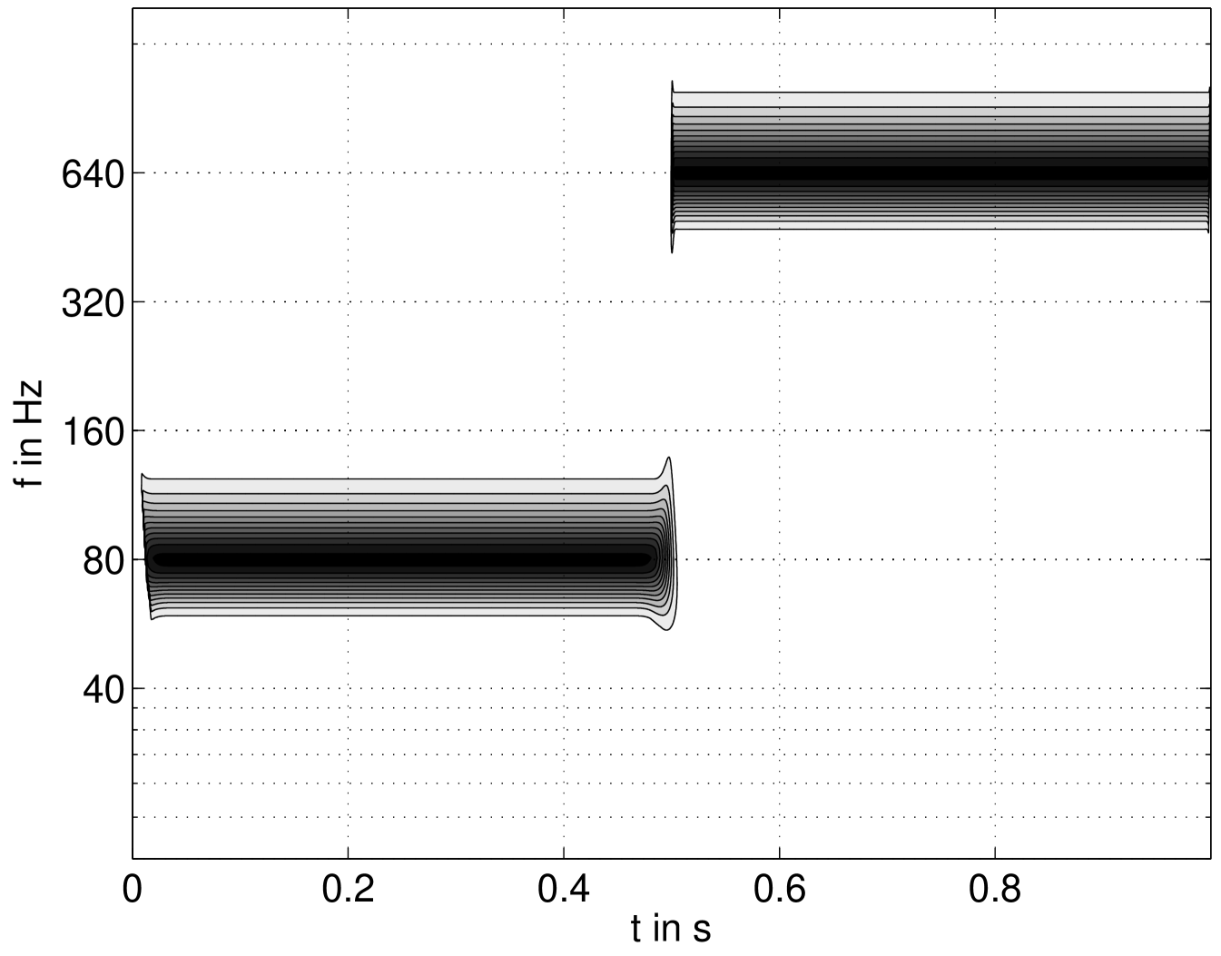
The peaks are very broad which is expected and due to the $e^{-\beta/2t^{2}}$ windowing term. The peak at $f_{1}=80Hz$ is lower than that at $640Hz$ , which is due to the truncation described above and that is plotted in figure 2. The peak value does not match the amplitude. This is due to the fact that the total power is approximately correct. Since the peak is very broad only the peak value or the total can power can be correct. The total power is $P=\sum_{i}P_{i}=8.1$ which corresponds to the correct value of $P=1/2A^{2}=8$ . Using the equal amplitude wavelet power spectrum that is given in equation (9) and performing an integration over time results in a good approximation of the peak value.
The energy density spectrum is plotted in the bottom part of figure 1, showing an unusual representation of the example equation (17).
A contour plot of the power density spectrum over time is given in figure 2. Note that the high frequency component $f_{2}$ is more accurately localized in the time domain.

Refer to caption — Figure 1: Power density spectrum equation (11) and energy density spectrum of equation (17) built with the Morlet wavelet

4.2 Energy signal

The tested signal is

y(t)=\frac{\sin(a/t)}{t}\mbox{ for }t_{min}<t<t_{max},

(18)

thereby, the parameters are set to $a=10$ , $1/\Delta t=f_{s}=2^{12}$ , $t_{min}=\sqrt{a/(2\pi f_{max})}$ , $f_{max}=f_{s}/8$ and $t_{max}=.25s$ .
The energy is plotted in figure 3. The solid curve is calculated with the discrete Fourier transform (DFT) and equation (14). The Fourier transform of function (18) can be obtained by the convolution of the Bessel-function $J_{0}$ which is the Fourier transform of $\frac{\sin(a/t)}{t}$ and the sinc-function which is the Fourier transform of the rectangular window of the size $T=t_{max}-t_{min}$ .

F\{y(t)\}=\frac{\pi}{2}J_{0}(2\sqrt{a\omega})\ast\frac{\sin(T\omega)}{\omega}.

(19)

The small fluctuations in figure 3 correspond to the sinc-function and the high and long to the Bessel-function.
The dashed curve is calculated with the Morlet wavelet transform. This curve follows more clearly the theoretical $1/\sqrt{\omega}$ dependence that is plotted as the dash dotted curve next to the others.
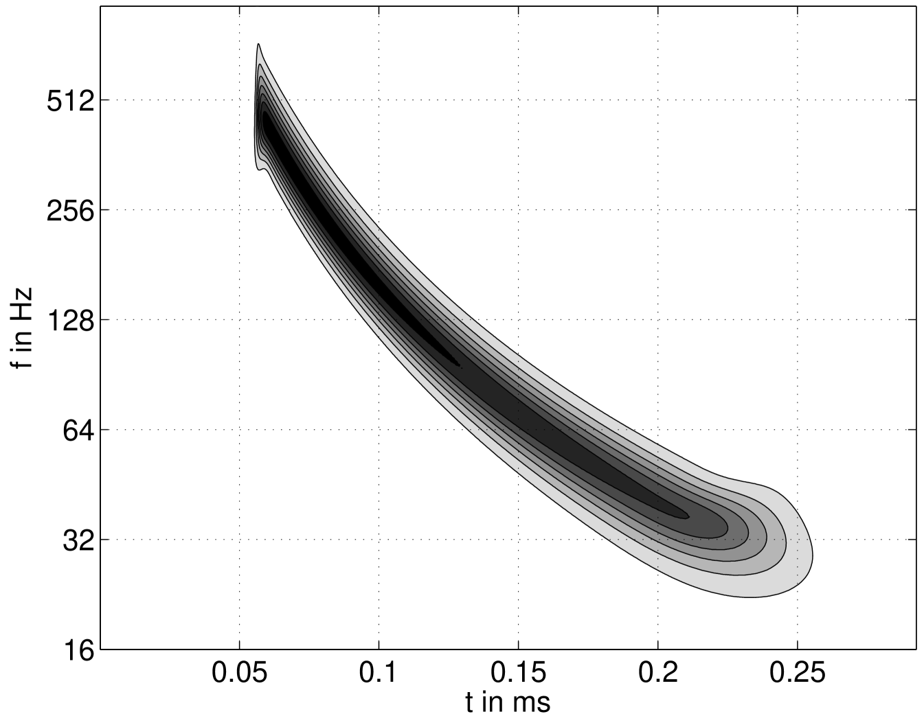
A contour plot of the energy density spectrum over time is given in figure 4. It shows good agreement with the actual frequency of this function which is given by $\omega(t)=a/t^{2}$ .

5 Concluding remarks

The study shows that it is possible to obtain an efficient transform with an algorithm that is restricted to the values that are numerically significant. This efficiency results in less computational effort and less memory consumption. Nevertheless, for applications that are time critical it will be worth to work on a optimized version in a native language and to apply optimisation. Since the programme is tested and open source, it will facilitate the programming of such an optimised version.
The examples and definitions of energy and power values should help with the interpretation of the values obtained with the wavelet transform.

References

[1] T. Önsay, A. G. Haddow, Wavelet transform analysis of transient wave propagation in a dispersive medium, Acoustical Society of America Journal 95 (1994) 1441–1449.
[2] K. Kishimoto, M. H. H. Inoue, T. Shibuya, Time frequency analysis of dispersive waves by means of wavelet transform, Journal of Applied Mechanics 62 (1995) 841–46.
[3] L. Gaul, S. Hurlebaus, Identification of the impact location on a plate using wavelets, Mechanical Systems and Signal Processing 12 (6) (1998) 783–795.
[4] C. Junsheng, Y. Dejie, Y. Yu, Application of an impulse response wavelet to fault diagnosis of rolling bearings, Mechanical Systems and Signal Processing 21 (2005) 920–929.
[5] Y. Hayashi, S. Ogawa, H. Cho, M. Takemoto, Non-contact estimation of thickness and elastic properties of metallic foils by the wavelet transform of laser-generated lamb waves, NDT & E international 32/1 (1998) 21–27.
[6] M.-N. Ta, J. Lardies, Identification of weak nonlinearities on damping and stiffness by the continuous wavelet transform, Journal of Sound and Vibration 293 (1) (2006) 16–37.
[7] P. Masson, A. Berry, P. Micheau, A wavelet approach for the active structural acoustic control, Journal of the Acoustical Society of America 104 (3) (1998) 1453–1466.
[8] Y. Kim, E. Kim, Effectiveness of the continuous wavelet transform in the analysis of some dispersive elastic waves, Journal of the Acoustical Society of America 110 (1) (2001) 86–94.
[9] M. Rucka, K. Wilde, Application of continuous wavelet transform in vibration based damage detection method for beams and plates, Journal of Sound and Vibration 297 (2006) 536–550.
[10] Q. Wang, X. Deng, Damage detection with spatial wavelets, International Journal of Solids and Structures 36 (1999) 3443–3468.
[11] A. Caprioli, A. Cigada, D. Raveglia, Rail inspection in track maintenance: A benchmark between the wavelet approach and the more conventional fourier analysis, Mechanical Systems and Signal Processing 21 (2007) 631–652.
[12] P. Loughlin, L. Cohen, A wigner approximation method for wave propagation, Journal of the Acoustical Society of America 118 (3) (2005) 1268–1271.
[13] J. C. Hong, K. H. Sun, Y. Y. Kim, Dispersion-based short-time fourier transform applied to dispersive waves, Journal of the Acoustical Society of America 117 (5) (2005) 2949–2960.
[14] S. A. Fulop, K. Fitz, Algorithms for computing the time-corrected instaneous frequency (reassigned) spectrogram, with applications, Journal of the Acoustical Society of America 199 (1) (2006) 360–371.
[15] S. Mallat, A wavelet tour of signal processing, Academic Press, 1998.
[16] A. Louis, P. Maaß, A. Rieder, Wavelets, B.G. Teubner, 1994.
[17] E. Schukin, R. Zamaraev, L. Schukin, The optimisation of wavelet transform for the impulse analysis in vibration signals, Mechanical Systems and Signal Processing 18 (2004) 1315–1333.
[18] V. Perrier, T. Philipovitch, C. Basdevant, Wavelet spectra compared to Fourier spectra, Journal of Mathematical Physics 36 (3) (1995) 1506–1519.
[19] H.-C. Shyun, Y.-S. Sun, Construction of a morlet wavelet power spectrum, Multidimensional Systems and Signal Processing 13 (2002) 101–111.
[20] H. Suzuki, T. Kinjo, Y. Hayashi, M. Takemoto, K. Ono, Wavelet transform of acoustic emission signals, Journal of Acoustic Emission 14/2 (1996) 69–84.
[21] D. Jordan, R. W. Miksad, E. J. Powers, Implementation of the continuous wavelet transform for digital time series analysis, Review of Scientific Instruments 68 (3) (1997) 1484–1494.
[22] J. E. Moreira, S. P. Midkiff, M. Gupta, From flop to megaflops: Java for technical computing, ACM Transactions on Programming Languages and Systems (TOPLAS) 22 (2) (2000) 265 – 295.