An analogy of Jacobi’s formula and its applications

Chiba Jun NEC Corporation, 7-1, Shiba 5-chome Minato-ku, Tokyo 108-8001, Japan jun.chiba323@nec.com and Matsumoto Keiji Department of Mathematics, Faculty of Science, Hokkaido University, Sapporo 060-0810, Japan matsu@math.sci.hokudai.ac.jp

Abstract.

We give an analogy of Jacobi’s formula, which relates the hypergeometric function with parameters $(1/4,1/4,1)$ and theta constants. By using this analogy and twice formulas of theta constants, we obtain a transformation formula for this hypergeometric function. As its application, we express the limit of a pair of sequences defined by a mean iteration by this hypergeometric function.

Key words and phrases:

Hypergeometric Function, Theta constants, Mean iteration.

2010 Mathematics Subject Classification:

Primary 33C05; Secondary 14K25, 33C90.

1. Introduction

Jacobi’s formula in elliptic function theory is an equality

F(\frac{1}{2},\frac{1}{2},1;\lambda(\tau))=\vartheta_{00}(\tau)^{2},\quad\lambda(\tau)=\frac{\vartheta_{10}(\tau(z))^{4}}{\vartheta_{00}(\tau(z))^{4}},

as holomorphic functions on the upper half plane $\mathbb{H}=\{\tau\in\mathbb{C}\mid\mathrm{Im}(\tau)>0\}$ , where $F(a,b,c;z)$ and $\vartheta_{pq}(\tau)$ denote the hypergeometric series on $\{z\in\mathbb{C}\mid|z|<1\}$ and the theta constant with characteristics $p,q\in\{0,1\}$ on $\mathbb{H}$ , respectively; refer to (2.1) and (3.1) for their definitions. This formula is applied to the study of the arithmetic-geometric mean as shown in [BB], and generalized to Thomae’s formula in [Th]. In the present, there are several kinds of its analogies, which are applied to studies of mean iterations, refer to [BB], [MS], [MT], [Sh] and the references therein.

In this paper, we give an analogy of Jacobi’s formula, which is an equality

F(\frac{1}{4},\frac{1}{4},1;\zeta(\tau))=\vartheta_{00}(\tau)^{2},\quad\zeta(\tau)=\frac{4\vartheta_{01}(\tau)^{4}\vartheta_{10}(\tau)^{4}}{\vartheta_{00}(\tau)^{8}},

as holomorphic functions on $\mathbb{H}$ . Strictly, we initially give this equality on a fundamental region $\mathbb{D}_{12}$ of

\Gamma_{12}=\{g=g_{ij}\in\mathrm{SL}_{2}(\mathbb{Z})\mid g_{11}g_{12},g_{21}g_{22}\equiv 0\bmod 2\}

acting on $\mathbb{H}$ , and extend it to the whole space $\mathbb{H}$ . Though this equality is naturally extended to $\mathbb{H}$ by the simply connectedness of $\mathbb{H}$ , $F(\frac{1}{4},\frac{1}{4},1;z)$ is not regarded as single valued when $\tau$ runs over $\mathbb{H}$ . To understand its behavior well, we investigate the monodromy representation of the hypergeometric differential equation $\mathcal{F}(\frac{1}{4},\frac{1}{4},1)$ . It is realized in not $\mathrm{SL}_{2}(\mathbb{Z})$ but $\mathrm{GL}_{2}(\mathbb{Z}[\mathbf{i}])$ , and its projectivization becomes $\mathrm{P}\Gamma_{12}=\Gamma_{12}/\{\pm I_{2}\}$ , where $\mathbf{i}=\sqrt{-1}$ and $I_{2}$ is the unit matrix of size $2$ . By using circuit matrices in $\mathrm{GL}_{2}(\mathbb{Z}[\mathbf{i}])$ , we can simplify not only the formula for $\vartheta_{00}(\tau)$ with respect to the action $\mathrm{P}\Gamma_{12}$ in Fact 3.3 but also a description of the behavior of $F(\frac{1}{4},\frac{1}{4},1;\tau(z))$ ; for details refer to Lemma 4.3 and Corollary 4.7. We also remark that the monodromy representation of $\mathcal{F}(\frac{1}{2},\frac{1}{2},1)$ is realized as

\Gamma(2,4)=\{g=(g_{ij})\in\mathrm{SL}_{2}(\mathbb{Z})\mid g_{11},\gamma_{22}\equiv 1\bmod 4,g_{12},g_{21}\equiv 0\bmod 2\},

which is a subgroup in $\Gamma(2)=\{g\in\mathrm{SL}_{2}(\mathbb{Z})\mid g\equiv I_{2}\bmod 2\}$ of index $2$ , and that there is a similar advantage in using not $\mathrm{P}\Gamma(2)=\Gamma(2)/\{\pm I_{2}\}$ but $\Gamma(2,4)$ for Jacobi’s formula, see Lemma 4.3 and Corollary 4.4.

By using our analogy of Jacobi’s formula together with twice formulas for theta constants in (3.3), we obtain a transformation formula for $F(\frac{1}{4},\frac{1}{4},1;z)$ in Theorem 5.1. As studied in [Go], [HKM], [KS1], [KS2] and [Ma], some transformation formulas for hypergeometric functions are applied to expressing limits of mean iterations. By following the idea in [HKM], we define two functions on the set

\mathbb{S}_{(-1,\infty)}=\{(x,rx)\in\mathbb{R}^{2}\mid x>0,\ -1<r<\infty\}

\mu_{1}(x,y)=m_{A}(x,\mu_{0}(x,y)),\quad\mu_{2}=\nu(x,\mu_{0}(x,y)),

where $m_{A}$ , $m_{G}$ and $m_{H}$ are the arithmetic, geometric and harmonic means, and

\mu_{0}=m_{G}(x,m_{A}(x,y)),\quad\nu(x,y)=2m_{H}(x,y)-m_{A}(x,y).

We can easily see that $\mu_{1}(x,y)$ is a mean on $\mathbb{S}_{(-1,\infty)}$ , however $\mu_{2}(x,y)$ is not, since the inequality $\min(x,y)\leq\mu_{2}(x,y)$ does not hold for any $(x,y)\in\mathbb{S}_{(-1,\infty)}$ . In spite of this situation, we can define a pair of sequences $\{x_{n}\}$ and $\{y_{n}\}$ by the recurrence relation

(x_{n+1},y_{n+1})=(\mu_{1}(x_{n},y_{n}),\mu_{2}(x_{n},y_{n}))

for any given initial term $(x_{0},y_{0})\in\mathbb{S}_{(-1,\infty)}$ , and show in Lemma 6.12 that they converge as $n\to\infty$ and $\lim\limits_{n\to\infty}x_{n}=\lim\limits_{n\to\infty}y_{n}>0$ . We express this limit by $F(\frac{1}{4},\frac{1}{4},1;z)$ in Theorem 6.13.

2. Fundamental properties of $F(a,b,c;z)$

We begin with defining the hypergeometric series.

Definition 2.1.

The hypergeometric series $F(a,b,c;z)$ is defined by

F(a,b,c;z)=\sum_{n=0}^{\infty}\frac{(a,n)(b,n)}{(c,n)(1,n)}z^{n},

(2.1)

where $z$ is a complex variable, $a,b,c$ are complex parameters with $c\neq 0,-1,-2,\cdots$ , and $(a,n)=\mathit{\Gamma}(a+n)/\mathit{\Gamma}(a)=a(a+1)\cdots(a+n-1)$ . It converges absolutely and uniformly on any compact set in the unit disk $\{z\in\mathbb{C}\mid|z|<1\}$ for any fixed $a,b,c$ .

This series satisfies the hypergeometric differential equation

\mathcal{F}(a,b,c):\big{[}z(1-z)\frac{d^{2}}{dz^{2}}+\{c-(a+b+1)z\}\frac{d}{dz}-ab\big{]}\cdot f(z)=0,

which is a second order linear ordinary differential equation with regular singular points $z=0,1,\infty$ . The space $\mathcal{S}(a,b,c;\dot{z})$ of local solutions to $\mathcal{F}(a,b,c)$ around a point $\dot{z}\in Z=\mathbb{C}-\{0,1\}$ is a $2$ -dimensional complex vector space, its element admits the analytic continuation along any path in $Z$ . In particular, a loop $\rho$ in $Z$ with a base point $\dot{z}$ leads to a linear transformation of $\mathcal{S}(a,b,c;\dot{z})$ . Thus, we have a homomorphism from the fundamental group $\pi_{1}(Z,\dot{z})$ to the general linear group $\mathrm{GL}(\mathcal{S}(a,b,c;\dot{z}))$ of $\mathcal{S}(a,b,c;\dot{z})$ , which is called the monodromy representation of $\mathcal{F}(a,b,c)$ . We take $\dot{z}=\frac{1}{2}$ as a base point of $Z$ , and loops $\rho_{0}$ and $\rho_{1}$ with terminal $\dot{z}$ as positively oriented circles with radius $\frac{1}{2}$ and center $0$ and $1$ , respectively. Since $\pi_{1}(Z,\dot{z})$ is a free group generated by $\rho_{0}$ and $\rho_{1}$ , the monodromy representation of $\mathcal{F}(a,b,c)$ is uniquely characterized by the images of $\rho_{0}$ and $\rho_{1}$ . We give their explicit forms with respect to a basis of $\mathcal{S}(a,b,c;\dot{z})$ given by Euler type integrals.

Fact 2.2 ([Ki, §17]).

(

i

)

If $\mathrm{Re}(b),\mathrm{Re}(c-b),\mathrm{Re}(1-a)>0$ then the integrals

f_{1}(z)=\int_{1}^{1/z}t^{b-1}(1-t)^{c-b-1}(1-tz)^{-a}dt,\quad f_{2}(z)=\int_{0}^{1}t^{b-1}(1-t)^{c-b-1}(1-tz)^{-a}dt

converge and span the space $\mathcal{S}(a,b,c;\dot{z})$ . Here we assign a branch of the integrand $t^{b-1}(1-t)^{c-b-1}(1-tz)^{-a}$ on the open interval $(0,1)$ in the $t$ -space by $\arg(t)=\arg(1-t)=\arg(1-tz)=0$ for real $z$ near to $\dot{z}=\frac{1}{2}$ , and that on the open interval $(1,\frac{1}{z})$ by its analytic continuation via the lower half plane of the $t$ -space, which transforms $\arg(1-t)$ from $0$ to $\pi$ . Under some generic conditions on $a,b,c$ , they admit expressions in terms of the hypergeometric series

	$\displaystyle f_{1}(z)$	$\displaystyle=e^{\pi\mathbf{i}(c-b-1)}B(c-b,1-a)(1-z)^{c-a-b}F(c-a,c-b,c-a-b+1;1-z),$
		$\displaystyle=\frac{e^{2\pi\mathbf{i}(c-b)}\!-\!e^{2\pi\mathbf{i}a}}{e^{2\pi\mathbf{i}a}\!-\!1}\left(B(b,c\!-\!b)F(a,b,c;z)\!-\!B(b,c\!-\!a\!-\!b)F(a,b,a\!+\!b\!-\!c\!+\!1;1\!-\!z)\right),$
	$\displaystyle f_{2}(z)$	$\displaystyle=B(b,c-b)F(a,b,c;z),$

where $B$ denotes the beta function.

(

ii

)

The loops $\rho_{0}$ and $\rho_{1}$ lead to linear transformations sending the basis $\mathbf{F}(z)=\;^{t}(f_{1}(z),f_{2}(z))$ of $\mathcal{S}(a,b,c;\dot{z})$ to $M_{0}\mathbf{F}(z)$ and $M_{1}\mathbf{F}(z)$ , where

M_{0}=\begin{pmatrix}e^{-2\pi\mathbf{i}c}&e^{-2\pi\mathbf{i}b}-1\\ 0&1\end{pmatrix},\quad M_{1}=\begin{pmatrix}e^{2\pi\mathbf{i}(c-a-b)}&0\\ 1-e^{-2\pi\mathbf{i}a}&1\end{pmatrix}.

(2.2)

Here we exchange the role of $f_{1}(z)$ and $f_{2}(z)$ in [Ki, §17], our matrices $M_{0}$ and $M_{1}$ are the conjugates of $A_{0}$ and $A_{1}$ in [Ki, p.123] by $U=\begin{pmatrix}0&1\\ 1&0\end{pmatrix}$ , respectively.

Remark 2.3.

We can make the analytic continuation of the hypergeometric series $F(a,b,c;z)$ to the simply connected domain $\mathbb{C}-[1,\infty)$ as a solution to $\mathcal{F}(a,b,c)$ . We use the same symbol $F(a,b,c;z)$ for this continuation, which is a single-valued holomorphic function on $\mathbb{C}-[1,\infty)$ . Moreover, by assigning $F(a,b,c;t)$ on $t\in(1,\infty)$ to the limit of $F(a,b,c;z)$ as $z\to t$ with $\mathrm{Im}(z)>0$ , we extend $F(a,b,c;z)$ to a single-valued function on $\mathbb{C}-\{1\}$ , which is discontinuous along $(1,\infty)$ for general $a,b,c$ . For a path $\rho$ in $Z=\mathbb{C}-\{0,1\}$ ending at $w$ , $F_{\rho}(a,b,c;w)$ denotes the continuation of $F(a,b,c;z)$ along $\rho$ .

Though we remove the point $z=1$ from $\mathbb{C}$ for $F(a,b,c;z)$ in Remark 2.3, there is a formula for the limit of $F(a,b,c;z)$ as $z\to 1$ with $z$ in the unit disk.

Fact 2.4 (Gauss-Kummer’s identity [Ki, Theorem 3.3]).

If $\mathrm{Re}(c-a-b)>0$ then

\lim_{z\to 1,|z|<1}F(a,b,c;z)=\frac{\mathit{\Gamma}(c)\mathit{\Gamma}(c-a-b)}{\mathit{\Gamma}(c-a)\mathit{\Gamma}(c-b)}.

(2.3)

For the basis $\mathbf{F}(z)=\;^{t}(f_{1}(z),f_{2}(z))$ of $\mathcal{S}(a,b,c;\dot{z})$ , we have a map from a neighborhood of $\dot{z}$ to the complex projective line $\mathbb{P}^{1}$ by the ratio $f_{1}(z)/f_{2}(z)$ of $f_{1}(z)$ and $f_{2}(z)$ . Schwarz’s map is define by its analytic continuation to $\mathbb{C}-\{0,1\}$ , which is multi valued in general.

Fact 2.5.

If the parameters $a,b,c$ are real and satisfy

\frac{1}{|1-c|},\frac{1}{|c-a-b|},\frac{1}{|a-b|}\in\{2,3,4\dots\}\cup\{\infty\},\quad|1-c|+|c-a-b|+|a-b|<1,

then the image of Schwarz’s map is isomorphic to an open dense subset of the upper half plane $\mathbb{H}=\{\tau\in\mathbb{C}\mid\mathrm{Im}(\tau)>0\}$ and its inverse is single valued. The projectivization of the image of its monodromy representation is conjugate to a discrete subgroup of $\mathrm{PSL}_{2}(\mathbb{R})=\mathrm{SL}_{2}(\mathbb{R})/\{\pm I_{2}\}$ generated by two elements $g_{0}$ and $g_{1}$ with

\mathrm{ord}(g_{0})=\frac{1}{|1-c|},\quad\mathrm{ord}(g_{1})=\frac{1}{|c-a-b|},\quad\mathrm{ord}(g_{0}^{-1}g_{1}^{-1})=\frac{1}{|a-b|},

where $I_{2}$ is the unit matrix of size $2$ , and $\mathrm{ord}(g_{0})$ denotes the order of $g_{0}$ .

Example 2.6.

If $(a,b,c)=(\frac{1}{2},\frac{1}{2},1)$ then we have $\big{(}\frac{1}{|1-c|},\frac{1}{|c-a-b|},\frac{1}{|a-b|}\big{)}=(\infty,\infty,\infty)$ ,

M_{0}=\begin{pmatrix}1&-2\\ 0&1\end{pmatrix},\quad M_{1}=\begin{pmatrix}1&0\\ 2&1\end{pmatrix},\quad M_{0}^{-1}M_{1}^{-1}=\begin{pmatrix}-3&2\\ -2&1\end{pmatrix}.

The group generated by these matrices is not the principal congruence subgroup $\Gamma(2)$ of level $2$ in $\mathrm{SL}_{2}(\mathbb{Z})$ but

\Gamma(2,4)=\{g=(g_{ij})\in\mathrm{SL}_{2}(\mathbb{Z})\mid g_{11},g_{22}\equiv 1\bmod 4,g_{12},g_{21}\equiv 0\bmod 2\}.

Note that $\Gamma(2,4)$ is a subgroup in $\Gamma(2)$ of index $2$ , and that $\pm I_{2}$ are representatives of the quotient $\Gamma(2)/\Gamma(2,4)$ .

Since the image of the monodromy representation is in $\mathrm{PSL}_{2}(\mathbb{R})$ and $f_{1}(z)/f_{2}(z)$ is in $\mathbb{H}$ for $z\in(0,1)$ , the image of the analytic continuation of $f_{1}(z)/f_{2}(z)$ to $Z=\mathbb{C}-\{0,1\}$ is the whole space $\mathbb{H}$ .

Example 2.7.

If $(a,b,c)=(\frac{1}{4},\frac{1}{4},1)$ then we have $\big{(}\frac{1}{|1-c|},\frac{1}{|c-a-b|},\frac{1}{|a-b|}\big{)}=(\infty,2,\infty)$ ,

M_{0}=\begin{pmatrix}1&-1-\mathbf{i}\\ 0&1\end{pmatrix},\quad M_{1}=\begin{pmatrix}-1&0\\ 1+\mathbf{i}&1\end{pmatrix},\quad M_{0}^{-1}M_{1}^{-1}=\begin{pmatrix}-1+2\mathbf{i}&1+\mathbf{i}\\ 1+\mathbf{i}&1\end{pmatrix}.

By using

P=\begin{pmatrix}-1+\mathbf{i}&\mathbf{i}\\ 0&1\end{pmatrix},

we change the basis $\mathbf{F}(z)$ into $P\mathbf{F}(z)$ . Then

PM_{0}P^{-1}=\begin{pmatrix}1&2\\ 0&1\end{pmatrix},\quad PM_{1}P^{-1}=\begin{pmatrix}0&\mathbf{i}\\ -\mathbf{i}&0\end{pmatrix}=\mathbf{i}J,\quad PM_{0}^{-1}M_{1}^{-1}P^{-1}=\begin{pmatrix}2\mathbf{i}&\mathbf{i}\\ -\mathbf{i}&0\end{pmatrix}.

The group generated by these matrices is

\Gamma(2,4)\langle\mathbf{i}J\rangle=\{g\in\mathrm{GL}_{2}(\mathbb{Z}[\mathbf{i}])\mid g\in\Gamma(2,4)\textrm{ or }(\mathbf{i}J)g\in\Gamma(2,4)\}=\Gamma(2,4)\cup(\mathbf{i}J)\cdot\Gamma(2,4)

since

\begin{pmatrix}0&\mathbf{i}\\ -\mathbf{i}&0\end{pmatrix}\begin{pmatrix}1&2\\ 0&1\end{pmatrix}\begin{pmatrix}0&\mathbf{i}\\ -\mathbf{i}&0\end{pmatrix}=\begin{pmatrix}1&0\\ -2&1\end{pmatrix}.

Note that the projectivization of $\Gamma(2,4)\langle\mathbf{i}J\rangle$ is isomorphic to that of

\Gamma_{12}=\{g=(g_{ij})\in\mathrm{SL}_{2}(\mathbb{Z})\mid g_{11}g_{12}\equiv g_{21}g_{22}\equiv 0\bmod 2\}.

Since the image of the monodromy representation is in $\mathrm{PSL}_{2}(\mathbb{R})$ and $\big{(}(-1+\mathbf{i})f_{1}(z)+\mathbf{i}f_{2}(z)\big{)}/f_{2}(z)$ is in $\mathbb{H}$ for $z\in(0,1)$ , the image of the analytic continuation of $f_{2}(z)/f_{1}(z)$ to $Z=\mathbb{C}-\{0,1\}$ is a open dense subset of $\mathbb{H}$ .

It is known that $F(a,b,c;z)$ satisfies several kinds of transformation formulas with respect to variable changes. In this paper, we use the following.

Fact 2.8 ([Er, (24) in p.64, (18),(19) in p.112 of Vol.I]).

$\displaystyle F(a,b,2b;\frac{4z}{(1+z)^{2}})$	$\displaystyle=(1+z)^{2a}F(a,a-b+\frac{1}{2},b+\frac{1}{2};z^{2}),$	(2.4)
$\displaystyle F(a,b,\frac{a+b+1}{2};z)$	$\displaystyle=F(\frac{a}{2},\frac{b}{2},\frac{a+b+1}{2};4z(1-z))$	(2.5)
	$\displaystyle=(1-2z)F(\frac{a+1}{2},\frac{b+1}{2},\frac{a+b+1}{2};4z(1-z)),$	(2.6)

where $z$ is sufficiently near to $0$ and $(1+z)^{2a}$ takes the value $1$ at $z=0$ .

3. Fundamental properties of $\vartheta_{pq}(\tau)$

We next introduce theta constants and their properties by referring to [Er] and [Mu].

Definition 3.1.

The theta constant $\vartheta_{pq}(\tau)$ with characteristics $p,q$ is defined by

\vartheta_{pq}(\tau)=\sum_{n=-\infty}^{\infty}\exp\big{(}\pi\mathbf{i}(n+\frac{p}{2})^{2}\tau+2\pi\mathbf{i}(n+\frac{p}{2})\frac{q}{2}\big{)},

(3.1)

where $\tau$ is a variable in the upper half plane $\mathbb{H}$ , and $p,q$ are parameters taking the value $0$ or $1$ . It converges absolutely and uniformly on any compact set in $\mathbb{H}$ for any fixed $p,q$ .

There are four functions $\vartheta_{00}(\tau)$ , $\vartheta_{01}(\tau)$ , $\vartheta_{10}(\tau)$ , $\vartheta_{11}(\tau)$ ; the last one vanishes identically on $\mathbb{H}$ , and the rests satisfy Jacobi’s identity

\vartheta_{00}(\tau)^{4}=\vartheta_{01}(\tau)^{4}+\vartheta_{10}(\tau)^{4}

(3.2)

for any $\tau\in\mathbb{H}$ . We have twice formulas of them.

Fact 3.2 ([Er, (15) in p.373 of Vol.II]).

The theta constants satisfy twice formulas

\begin{array}[]{l}\vartheta_{00}(2\tau)^{2}=\dfrac{\vartheta_{00}(\tau)^{2}+\vartheta_{01}(\tau)^{2}}{2},\\[5.69054pt] \vartheta_{01}(2\tau)^{2}=\vartheta_{00}(\tau)\vartheta_{01}(\tau),\\[5.69054pt] \vartheta_{10}(2\tau)^{2}=\dfrac{\vartheta_{00}(\tau)^{2}-\vartheta_{01}(\tau)^{2}}{2}.\end{array}

(3.3)

Fact 3.3 ([Mu, Theorem 7.1]).

Let $g=(g_{ij})$ be an element in the projectivization $\mathrm{P}\Gamma_{12}$ of $\Gamma_{12}$ . By multiplying $-1$ to $g$ if necessary, we may assume that $g$ satisfies either $g_{21}>0$ , or $g_{21}=0$ and $g_{22}>0$ . Then we have

\vartheta_{00}(g\cdot\tau)^{2}=\chi(g)\cdot(g_{21}\tau+g_{22})\vartheta_{00}(\tau)^{2}

for any $\tau\in\mathbb{D}_{12}$ , where

\chi(g)=\left\{\begin{array}[]{lcc}\mathbf{i}^{g_{22}-1}&\textrm{if}&g_{21}\in 2\mathbb{Z},g_{22}\notin 2\mathbb{Z},\\ \mathbf{i}^{-g_{21}}&\textrm{if}&g_{21}\notin 2\mathbb{Z},g_{22}\in 2\mathbb{Z}.\end{array}\right.

Fact 3.4 ([Mu, Table V in p.36]).

We have

\vartheta_{00}(\frac{-1}{\tau})^{2}=(-\mathbf{i}\tau)\vartheta_{00}(\tau)^{2},\quad\vartheta_{01}(\frac{-1}{\tau})^{2}=(-\mathbf{i}\tau)\vartheta_{10}(\tau)^{2},\quad\vartheta_{10}(\frac{-1}{\tau})^{2}=(-\mathbf{i}\tau)\vartheta_{01}(\tau)^{2}.

Fact 3.5 (The inverse of Schwarz’s map).

(

i

)

[Yo, §5.6,5.7,5.8 in Chap. II, Proposition 8.1 in Chap. III] The inverse of Schwarz’s map

z\mapsto\tau=\frac{f_{1}(z)}{f_{2}(z)}=\mathbf{i}\cdot\frac{F(\frac{1}{2},\frac{1}{2},1,1-z)}{F(\frac{1}{2},\frac{1}{2},1,z)}

(3.4)

for $(a,b,c)=(\frac{1}{2},\frac{1}{2},1)$ is

\mathbb{H}\ni\tau\mapsto\lambda(\tau)=\frac{\vartheta_{10}(\tau)^{4}}{\vartheta_{00}(\tau)^{4}}\in Z.

The function $\lambda(\tau)$ is invariant under the action $\tau\mapsto(g_{11}\tau+g_{12})/(g_{21}\tau+g_{22})$ of $g=(g_{ij})\in\Gamma(2)$ on $\tau\in\mathbb{H}$ .

(

ii

)

[MOT, Theorem 8.4] The inverse of Schwarz’s map

$\displaystyle z\mapsto\tau=$	$\displaystyle\frac{(-1+\mathbf{i})f_{1}(z)+\mathbf{i}f_{2}(z)}{f_{2}(z)}$
$\displaystyle=$	$\displaystyle\mathbf{i}\cdot\frac{\pi F(\frac{1}{4},\frac{1}{4},1;z)+B(\frac{3}{4},\frac{3}{4})\sqrt{1-z}F(\frac{3}{4},\frac{3}{4},\frac{3}{2},1-z)}{\pi F(\frac{1}{4},\frac{1}{4},1,z)}$	(3.5)
$\displaystyle=$	$\displaystyle\mathbf{i}\cdot\frac{-\pi F(\frac{1}{4},\frac{1}{4},1;z)+B(\frac{1}{4},\frac{1}{4})F(\frac{1}{4},\frac{1}{4},\frac{1}{2},1-z)}{\pi F(\frac{1}{4},\frac{1}{4},1,z)},$

for $(a,b,c)=(\frac{1}{4},\frac{1}{4},1)$ is

\mathbb{H}\ni\tau\mapsto\zeta(\tau)=\frac{4\vartheta_{01}^{4}(\tau)\vartheta_{10}^{4}(\tau)}{\vartheta_{00}(\tau)^{8}}\in Z\cup\{1\}=\mathbb{C}-\{0\}.

The function $\zeta(\tau)$ is invariant under the action $\tau\mapsto(g_{11}\tau+g_{12})/(g_{21}\tau+g_{22})$ of $g=(g_{ij})\in\Gamma_{1,2}$ on $\tau\in\mathbb{H}$ .

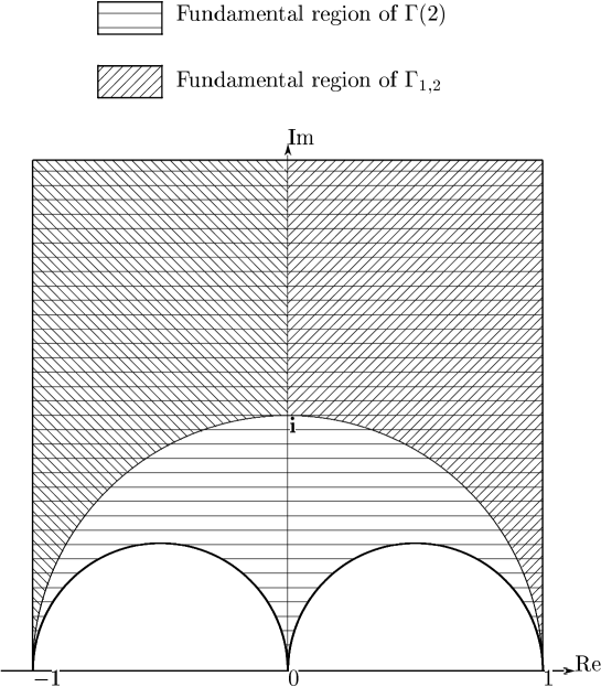
Here we give a fundamental region of $\Gamma(2)$ and that of $\Gamma_{12}$ as

	$\displaystyle\mathbb{D}(2)$	$\displaystyle=\{\tau\in\mathbb{H}\mid-1<\mathrm{Re}(\tau)\leq 1,\ \|\tau-\dfrac{1}{2}\|\geq\dfrac{1}{2},\ \|\tau+\dfrac{1}{2}\|>\dfrac{1}{2}\},$		(3.6)
	$\displaystyle\mathbb{D}_{12}$	$\displaystyle=\{\tau\in\mathbb{H}\mid-1<\mathrm{Re}(\tau)\leq 1,\ \|\tau\|>1\}\cup\{\tau\in\mathbb{H}\mid\|\tau\|=1,0\leq\mathrm{Re}(\tau)\leq 1\}.$		(3.7)

Refer to caption — Figure 1. Fundamental regions for $\Gamma(2)$ and $\Gamma_{12}$

4. Jacobi’s formula and its analogy

As given in [BB, Theorem 2.1], the hypergeometric series $F(\frac{1}{2},\frac{1}{2},1;x)$ and the theta constants are related by Jacobi’s formula:

Fact 4.1 (Jacobi’s formula).

Set

\lambda(\tau)=\frac{\vartheta_{10}(\tau)^{4}}{\vartheta_{00}(\tau)^{4}}

for any element $\tau$ in $\mathbb{D}(2)$ . Then Jacobi’s formula

F(\frac{1}{2},\frac{1}{2},1;\lambda(\tau))=\vartheta_{00}(\tau)^{2}

(4.1)

holds, where $F(\frac{1}{2},\frac{1}{2},1;z)$ denotes the single-valued function on $\mathbb{C}-\{1\}$ given in Remark 2.3. By the restriction of Schwarz’s map

z\mapsto\tau=\tau(z)=\mathbf{i}\frac{F(\frac{1}{2},\frac{1}{2},1;1-z)}{F(\frac{1}{2},\frac{1}{2},1;z)}

in (3.4) to the domain $\{z\in\mathbb{C}\mid|z|<1,\ |z-1|<1\}$ , the equality (4.1) is pulled back to

F(\frac{1}{2},\frac{1}{2},1;z)=\theta_{00}(\tau(z))^{2}.

(4.2)

Remark 4.2.

Suppose that $\tau$ is in the interior $\mathbb{D}(2)^{\circ}$ of $\mathbb{D}(2)$ .

( $i$ )

If $\mathrm{Re}(\tau)\geq 0$ then $\mathrm{Im}(\lambda(\tau))\geq 0$ , otherwise $\mathrm{Im}(\lambda(\tau))<0$ .
( $ii$ )

If $\tau$ approaches to a point in the boundary components $\{\tau\in\mathbb{H}\mid\mathrm{Re}(\tau)=\pm 1\}$ of $\mathbb{D}(2)$ , then $\lambda(\tau)$ converges to a negative real value, at which the hypergeometric series is naturally extended.
( $iii$ )

If $\tau$ approaches to a point in the boundary component $\{\tau\in\mathbb{H}\mid|\tau-\frac{1}{2}|=\frac{1}{2}\}$ of $\mathbb{D}(2)$ , then $\lambda(\tau)$ approaches to a real value greater than $1$ via the upper half plane. Note that the addition of this component to $\mathbb{D}(2)$ is compatible with the definition of $F(a,b,c;z)$ on $\mathbb{C}-\{1\}$ in Remark 2.3.

To extend (4.1) to the formula on the whole space $\mathbb{H}$ , we need to consider the continuation of $F(\frac{1}{2},\frac{1}{2},1;\lambda(\tau))$ . We prepare a lemma.

Lemma 4.3.

For $g=(g_{ij})\in\Gamma(2,4)\langle\mathbf{i}J\rangle$ , let $g^{\prime}=(g^{\prime}_{ij})\in\mathrm{P}\Gamma_{12}$ be its normalization of $g$ in the formula of Fact 3.3. Then we have

g_{21}\tau+g_{22}=\chi(g^{\prime})\cdot(g^{\prime}_{21}\tau+g^{\prime}_{22}).

Proof..

At first, we consider the case $g=(g_{ij})\in\Gamma(2,4)$ . In this case, we have $g_{22}\equiv 1\bmod 4$ . If $g_{21}>0$ then $g^{\prime}=g$ and

\chi(g^{\prime})\cdot(g^{\prime}_{21}\tau+g^{\prime}_{22})=\mathbf{i}^{g_{22}-1}\cdot(g_{21}\tau+g_{22})=g_{21}\tau+g_{22}.

If $g_{21}<0$ then $g^{\prime}=-g$ and

\chi(g^{\prime})\cdot(g^{\prime}_{21}\tau+g^{\prime}_{22})=\mathbf{i}^{-g_{22}-1}\cdot(-g_{21}\tau-g_{22})=g_{21}\tau+g_{22}.

If $g_{21}=0$ then $g^{\prime}_{22}=|g_{22}|$ and

\chi(g^{\prime})\cdot(g^{\prime}_{21}\tau+g^{\prime}_{22})=\mathbf{i}^{|g_{22}|-1}\cdot|g_{22}|=\left\{\begin{array}[]{ccc}\mathbf{i}^{g_{22}-1}\cdot g_{22}=g_{22}&\textrm{if}&g_{22}>0,\\ \mathbf{i}^{-g_{22}-1}\cdot(-g_{22})=g_{22}&\textrm{if}&g_{22}<0.\end{array}\right.

Next we consider the case $g=(g_{ij})\in(\mathbf{i}J)\cdot\Gamma(2,4)$ . In this case, $g_{21}$ takes the form of $(-\mathbf{i})\cdot(4m+1)$ ( $m\in\mathbb{Z}$ ), and $g^{\prime}$ is given by a scalar multiplication of $\pm\mathbf{i}$ to $g$ with $g_{21}^{\prime}=|4m+1|$ . Since they do not vanish, it is sufficient to show $\chi(g^{\prime})\cdot g^{\prime}_{21}=g_{12}$ . In fact, we have

\chi(g^{\prime})\cdot g^{\prime}_{21}=|4m+1|\cdot\mathbf{i}^{-|4m+1|}=\left\{\begin{array}[]{rll}(4m+1)\cdot\mathbf{i}^{-(4m+1)}=(-\mathbf{i})\cdot(4m+1)&\textrm{if}&4m+1>0,\\ -(4m+1)\cdot\mathbf{i}^{4m+1}=(-\mathbf{i})\cdot(4m+1)&\textrm{if}&4m+1<0.\end{array}\right.

Thus $g_{21}\tau+g_{22}=\chi(g^{\prime})\cdot(g^{\prime}_{21}\tau+g^{\prime}_{22})$ holds in any cases. $\square$

Corollary 4.4.

We extend Jacobi’s formula (4.1) to the equality on the whole space $\mathbb{H}$ as

	$\displaystyle\vartheta_{00}(\tau)^{2}=$	$\displaystyle F_{\rho}(\frac{1}{2},\frac{1}{2},1;\lambda(\tau))$		(4.3)
	$\displaystyle=$	$\displaystyle(g_{21}\tau_{0}+g_{22})F(\frac{1}{2},\frac{1}{2},1;\lambda(\tau_{0}))=\frac{F(\frac{1}{2},\frac{1}{2},1;\lambda(\tau))}{-g_{21}\tau+g_{11}},$		(4.4)

where $\tau$ is any element in $\mathbb{H}$ , $\tau_{0}\in\mathbb{D}(2)$ and $g=(g_{ij})\in\Gamma(2,4)$ satisfy

\tau=g\cdot\tau_{0}=\frac{g_{11}\tau_{0}+g_{12}}{g_{21}\tau_{0}+g_{22}},

$\rho$ is the image of a path from $\tau_{0}$ to $\tau$ in $\mathbb{H}$ under the map $\mathbb{H}\ni\tau\mapsto\lambda(\tau)\in\mathbb{C}-\{0,1\}$ , $F(\frac{1}{2},\frac{1}{2},1;z)$ denotes the single-valued function on $\mathbb{C}-\{1\}$ given in Remark 2.3, and $F_{\rho}(\frac{1}{2},\frac{1}{2},1;w)$ is its analytic continuation along $\rho$ .

Proof..

We obtain the identity (4.3) by the analytic continuation of (4.1) to $\mathbb{H}$ . We also have

	$\displaystyle\vartheta_{00}(\tau)^{2}=$	$\displaystyle\vartheta_{00}(g\cdot\tau_{0})^{2}=(g_{21}\tau_{0}+g_{22})\cdot\vartheta_{00}(\tau_{0})^{2}=(g_{21}\tau_{0}+g_{22})\cdot F(\frac{1}{2},\frac{1}{2},1;\lambda(\tau_{0}))$
	$\displaystyle=$	$\displaystyle(g_{21}\tau_{0}+g_{22})\cdot F(\frac{1}{2},\frac{1}{2},1;\lambda(\tau))=\frac{F(\frac{1}{2},\frac{1}{2},1;\lambda(\tau))}{-g_{21}\tau+g_{11}}$

by (4.1) and Lemma 4.3. Here note that

\tau_{0}=\frac{g_{22}\tau-g_{12}}{-g_{21}\tau+g_{11}},\quad g_{21}\tau_{0}+g_{22}=g_{21}\frac{g_{22}\tau-g_{12}}{-g_{21}\tau+g_{11}}+g_{22}=\frac{1}{-g_{21}\tau+g_{11}},

and that $\lambda(\tau)=\lambda(\tau_{0})$ . $\square$

We give an analogy of Jacobi’s formula (4.1).

Theorem 4.5.

We set

\zeta(\tau)=\frac{4\vartheta_{01}(\tau)^{4}\vartheta_{10}(\tau)^{4}}{\vartheta_{00}(\tau)^{8}}

for any $\tau$ in $\mathbb{D}_{12}$ . Then we have

	$\displaystyle F\Big{(}\frac{1}{4},\frac{1}{4},1;\zeta(\tau)\Big{)}=$	$\displaystyle\vartheta_{00}(\tau)^{2},$		(4.5)
	$\displaystyle F\Big{(}\frac{3}{4},\frac{3}{4},1;\zeta(\tau)\Big{)}=$	$\displaystyle\frac{\vartheta_{00}(\tau)^{6}}{\vartheta_{01}(\tau)^{4}-\vartheta_{10}(\tau)^{4}},$		(4.6)

where the hypergeometric series is extended to the single-valued function on $\mathbb{C}-\{1\}$ given in Remark 2.3.

Proof..

By substituting $a=b=1/2$ into (2.5), we have

F(\frac{1}{2},\frac{1}{2},1;\lambda)=F(\frac{1}{4},\frac{1}{4},1;4\lambda(1-\lambda)),

where $\lambda$ is sufficiently near to $0$ . Jacobi’s formula (4.1) together with Jacobi’s identity (3.2) yields that

	$\displaystyle\vartheta_{00}(\tau)^{2}$	$\displaystyle=F\Big{(}\frac{1}{2},\frac{1}{2},1;\frac{\vartheta_{10}(\tau)^{4}}{\vartheta_{00}(\tau)^{4}}\Big{)}=F\Big{(}\frac{1}{4},\frac{1}{4},1;4\frac{\vartheta_{10}(\tau)^{4}}{\vartheta_{00}(\tau)^{4}}\big{(}1-\frac{\vartheta_{10}(\tau)^{4}}{\vartheta_{00}(\tau)^{4}})\Big{)}$
		$\displaystyle=F\Big{(}\frac{1}{4},\frac{1}{4},1;\frac{4\vartheta_{01}(\tau)^{4}\vartheta_{10}(\tau)^{4}}{\vartheta_{00}(\tau)^{8}}\Big{)}$

for $\tau$ with sufficiently large imaginary part. We can extend this identity to any $\tau\in\mathbb{D}_{12}$ since if $\tau$ belongs to the interior of $\mathbb{D}_{12}$ then $\zeta(\tau)$ is in $\mathbb{C}-[1,\infty)$ on which $F(1/4,1/4,1;z)$ is single valued.

To show the second formula, use (2.6) with the substitution $a=b=1/2$ . Then we have

\vartheta_{00}(\tau)^{2}=\big{(}1-2\frac{\vartheta_{10}(\tau)^{4}}{\vartheta_{00}(\tau)^{4}}\big{)}F\Big{(}\frac{3}{4},\frac{3}{4},1;\zeta(\tau)\Big{)},

which is equivalent to (4.6). $\square$

Remark 4.6.

(

i

)

Substitute $\tau=\mathbf{i}$ into (4.5). Fact 3.4 implies $\vartheta_{01}(\mathbf{i})^{2}=\vartheta_{10}(\mathbf{i})^{2}$ , and Jacobi’s identity (3.2) becomes $\vartheta_{00}(\mathbf{i})^{4}=\vartheta_{01}(\mathbf{i})^{4}+\vartheta_{10}(\mathbf{i})^{4}=2\vartheta_{10}(\mathbf{i})^{4}$ . By Gauss-Kummer’s identity (2.3), we have

\vartheta_{00}(\mathbf{i})^{2}=F(\frac{1}{4},\frac{1}{4},1;\frac{4\vartheta_{01}(\mathbf{i})^{4}\vartheta_{10}(\mathbf{i})^{4}}{\vartheta_{00}(\mathbf{i})^{8}})=F(\frac{1}{4},\frac{1}{4},1;1)=\frac{\mathit{\Gamma}(1)\mathit{\Gamma}(\frac{1}{2})}{\mathit{\Gamma}(\frac{3}{4})\mathit{\Gamma}(\frac{3}{4})}=\Big{(}\frac{\pi^{1/4}}{\mathit{\Gamma}(\frac{3}{4})}\Big{)}^{2},\\

which yields

\vartheta_{00}(\mathbf{i})=\frac{\pi^{1/4}}{\mathit{\Gamma}(\frac{3}{4})}

since $\vartheta_{00}(\mathbf{i})$ is positive real.

( $ii$ )

The right hand side of (4.6) has a simple pole at $\tau=\mathbf{i}$ . Here note that we cannot apply Gauss-Kummer’s identity (2.3) to the left hand side of (4.6) for $\tau=\mathbf{i}$ since $c-a-b$ for $(a,b,c)=(\frac{3}{4},\frac{3}{4},1)$ is $1-\frac{3}{4}-\frac{3}{4}=-\frac{1}{2}<0$ .

We extend Theorem 4.5 to formulas for the whole space $\mathbb{H}$ .

Corollary 4.7.

The equalities (4.5) and (4.6) are extended to

		$\displaystyle\hskip 51.21504pt\begin{array}[]{ll}\vartheta_{00}(\tau)^{2}&=F_{\rho}(\frac{1}{4},\frac{1}{4},1;\zeta(\tau))\\ &=(g_{21}\tau_{0}+g_{22})F(\frac{1}{4},\frac{1}{4},1;\zeta(\tau_{0}))=\dfrac{\det(g)F(\frac{1}{4},\frac{1}{4},1;\zeta(\tau))}{-g_{21}\tau+g_{11}},\\ \end{array}$		(4.9)
		$\displaystyle\begin{array}[]{ll}\dfrac{\vartheta_{00}(\tau)^{6}}{\vartheta_{01}(\tau)^{4}-\vartheta_{10}(\tau)^{4}}&=F_{\rho}(\frac{3}{4},\frac{3}{4},1;\zeta(\tau))\\ &=\dfrac{g_{21}\tau_{0}+g_{22}}{\det(g)}F(\frac{3}{4},\frac{3}{4},1;\zeta(\tau_{0}))=\dfrac{F(\frac{3}{4},\frac{3}{4},1;\zeta(\tau))}{-g_{21}\tau+g_{11}},\end{array}$		(4.12)

where $\tau$ is any element in $\mathbb{H}$ , $\tau_{0}\in\mathbb{D}_{12}$ and $g=(g_{ij})\in\Gamma(2,4)\langle\mathbf{i}J\rangle$ satisfy

\tau=g\cdot\tau_{0}=\frac{g_{11}\tau_{0}+g_{12}}{g_{21}\tau_{0}+g_{22}},

$\rho$ is the image of a path $\tau_{0}$ to $\tau$ in $\mathbb{H}$ under the map $\mathbb{H}\ni\tau\mapsto\zeta(\tau)\in\mathbb{C}-\{1\}$ , $F(a,b,c;z)$ is extended to the single-valued function on $\mathbb{C}-\{1\}$ given in Remark 2.3, and $F_{\rho}(a,b,c;w)$ is its analytic continuation along $\rho$ .

Proof..

We can show

\vartheta_{00}(\tau)^{2}=F_{\rho}(\frac{1}{4},\frac{1}{4},1;\zeta(\tau))=(g_{21}\tau_{0}+g_{22})F(\frac{1}{4},\frac{1}{4},1;\zeta(\tau_{0}))

quite similarly to Proof of Corollary 4.4. Since

\det(g)=\left\{\begin{array}[]{rcl}1&\textrm{if}&g\in\Gamma(2,4),\\ -1&\textrm{if}&g\in(\mathbf{i}J)\cdot\Gamma(2,4),\end{array}\right.

we have

g_{21}\tau_{0}+g_{22}=\frac{1}{\det(g)(-g_{21}\tau+g_{11})}

for any $g\in\Gamma(2,4)\langle\mathbf{i}J\rangle$ , which leads to the last equality in (4.9).

To show (4.12), we have only to note that

	$\displaystyle\frac{\vartheta_{00}(\tau)^{6}}{\vartheta_{01}(\tau)^{4}-\vartheta_{10}(\tau)^{4}}$	$\displaystyle=\vartheta_{00}(g\cdot\tau_{0})^{2}\frac{\vartheta_{00}(g\cdot\tau_{0})^{4}}{\vartheta_{01}(g\cdot\tau_{0})^{4}-\vartheta_{10}(g\cdot\tau_{0})^{4}},$
	$\displaystyle\vartheta_{00}(g\cdot\tau_{0})^{2}$	$\displaystyle=(g_{21}\tau_{0}+g_{22})\vartheta_{00}(\tau_{0})^{2},$
	$\displaystyle\frac{\vartheta_{00}(g\cdot\tau_{0})^{4}}{\vartheta_{01}(g\cdot\tau_{0})^{4}-\vartheta_{10}(g\cdot\tau_{0})^{4}}$	$\displaystyle=\left\{\begin{array}[]{ccl}\dfrac{\vartheta_{00}(\tau_{0})^{4}}{\vartheta_{01}(\tau_{0})^{4}-\vartheta_{10}(\tau_{0})^{4}}&\textrm{if}&g\in\Gamma(2,4),\\[11.38109pt] \dfrac{\vartheta_{00}(\tau_{0})^{4}}{\vartheta_{10}(\tau_{0})^{4}-\vartheta_{01}(\tau_{0})^{4}}&\textrm{if}&g\in(\mathbf{i}J)\cdot\Gamma(2,4),\\ \end{array}\right.$

by (3.2) and Facts 3.3, 3.4, 3.5 ( $i$ ). $\square$

By regarding $\tau$ as a dependent variable of $z$ in the domain $\{z\in\mathbb{C}\mid|z|<1,\ |z-1|<1\}$ by Schwarz’s map (3.5), we rewrite Theorem 4.5 into the following.

Corollary 4.8.

By the restriction of Schwarz’s map $z\mapsto\tau(z)$ in (3.5) to the domain $\{z\in\mathbb{C}\mid|z|<1,\ |z-1|<1\}$ , the equalities (4.5), (4.6) are pulled back to

F(\frac{1}{4},\frac{1}{4},1;z)=\vartheta_{00}(\tau(z))^{2},\quad F(\frac{3}{4},\frac{3}{4},1;z)=\frac{\vartheta_{00}(\tau(z))^{6}}{\vartheta_{01}(\tau(z))^{4}-\vartheta_{10}(\tau(z))^{4}}.

5. A transformation formula for $F(\frac{1}{4},\frac{1}{4},1;z)$ .

Theorem 5.1.

We have a transformation formula

\frac{2+\sqrt{2+2w}}{4}F(\frac{1}{4},\frac{1}{4},1;1-w^{2})=F\Big{(}\frac{1}{4},\frac{1}{4},1;1-\frac{(6\sqrt{2w+2}-w-3)^{2}}{(2\sqrt{2w+2}+w+3)^{2}}\Big{)},

(5.1)

where $w$ is in a neighborhood of $1$ , and $\sqrt{2+2w}$ takes $2$ at $w=1$ .

Proof..

By substituting $2\tau$ into $\tau$ for (4.5), and using (3.3), we have

F(\frac{1}{4},\frac{1}{4},1;\zeta(2\tau))=\vartheta_{00}(2\tau)^{2}=\frac{\vartheta_{00}(\tau)^{2}+\vartheta_{01}(\tau)^{2}}{2}=\frac{\vartheta_{00}(\tau)^{2}+\vartheta_{01}(\tau)^{2}}{2\vartheta_{00}(\tau)^{2}}\cdot\vartheta_{00}(\tau)^{2},

(5.2)

where we restrict $\tau\in\mathbb{H}$ to pure imaginary numbers with sufficiently large imaginary part. Note that

	$\displaystyle\zeta(\tau)$	$\displaystyle=\frac{4\vartheta_{01}(\tau)^{4}\vartheta_{10}(\tau)^{4}}{\vartheta_{00}(\tau)^{8}}=1-\frac{(\vartheta_{01}(\tau)^{4}+\vartheta_{10}(\tau)^{4})^{2}-4\vartheta_{01}(\tau)^{4}\vartheta_{10}(\tau)^{4}}{\vartheta_{00}(\tau)^{8}}$
		$\displaystyle=1-\frac{(\vartheta_{01}(\tau)^{4}-\vartheta_{10}(\tau)^{4})^{2}}{\vartheta_{00}(\tau)^{8}}=1-\Big{(}\frac{2\vartheta_{01}(\tau)^{4}-\vartheta_{00}(\tau)^{4}}{\vartheta_{00}(\tau)^{4}}\Big{)}^{2}.$

Put

w=\frac{2\vartheta_{01}(\tau)^{4}-\vartheta_{00}(\tau)^{4}}{\vartheta_{00}(\tau)^{4}},

then we have

\vartheta_{01}(\tau)^{4}=\frac{w+1}{2}\cdot\vartheta_{00}(\tau)^{4},\quad\vartheta_{01}(\tau)^{2}=\frac{\sqrt{2w+2}}{2}\cdot\vartheta_{00}(\tau)^{2},

the last term of (5.2) is

\frac{\vartheta_{00}(\tau)^{2}+\vartheta_{01}(\tau)^{2}}{2\vartheta_{00}(\tau)^{2}}\cdot\vartheta_{00}(\tau)^{2}=\frac{2+\sqrt{2w+2}}{4}\cdot F(\frac{1}{4},\frac{1}{4},1;1-w^{2}),

which is the left hand side of (5.1). Here note that $\vartheta_{01}(\tau)>0$ for any pure imaginary number $\tau$ .

Let us express $\zeta(2\tau)$ in terms of $w$ . We have

	$\displaystyle\zeta(2\tau)$	$\displaystyle=1-\Big{(}\frac{2\vartheta_{01}(2\tau)^{4}-\vartheta_{00}(2\tau)^{4}}{\vartheta_{00}(2\tau)^{4}}\Big{)}^{2}=1-\Big{(}\frac{8\vartheta_{00}(\tau)^{2}\vartheta_{01}(\tau)^{2}-(\vartheta_{00}(\tau)^{2}+\vartheta_{01}(\tau)^{2})^{2}}{\vartheta_{00}(\tau)^{2}+\vartheta_{01}(\tau)^{2}}\Big{)}^{2}$
		$\displaystyle=1-\Big{(}\frac{16\sqrt{2w+2}-(2+\sqrt{2w+2})^{2}}{(2+\sqrt{2w+2})^{2}}\Big{)}^{2}=1-\Big{(}\frac{6\sqrt{2w+2}-w-3}{2\sqrt{2w+2}+w+3}\Big{)}^{2}.$

Hence $F(\frac{1}{4},\frac{1}{4},1;\zeta(2\tau))$ in (5.2) is equal to the right hand side of (5.1). $\square$

6. Mean iterations

By referring to [BB, Chapter 8], we give fundamental properties of mean iterations.

Definition 6.1 (Means).

A mean on a subset $\mathbb{S}$ in $\mathbb{R}^{2}$ is a continuous function $m$ defined on $\mathbb{S}$ satisfying

\min(x,y)\leq m(x,y)\leq\max(x,y)

(6.1)

for any $(x,y)\in\mathbb{S}$ .
A mean $m(x,y)$ is strict if it satisfies

m(x,y)=x\textrm{ or }m(x,y)=y\quad\Leftrightarrow\quad x=y.

(6.2)

A mean $m(x,y)$ is homogeneous if $\mathbb{S}$ and $m$ satisfy

(r\cdot x,r\cdot y)\in\mathbb{S},\quad m(r\cdot x,r\cdot y)=r\cdot m(x,y)

(6.3)

for any $(x,y)\in\mathbb{S}$ and any $r\in\mathbb{R}_{+}=\{x\in\mathbb{R}\mid x>0\}$ .
A mean $m(x,y)$ is symmetric if $\mathbb{S}$ and $m$ satisfy

(y,x)\in\mathbb{S},\quad m(y,x)=m(x,y)

(6.4)

for any $(x,y)\in\mathbb{S}$ .

We set the arithmetic mean on $\mathbb{R}^{2}$ , the geometric mean on $\mathbb{R}_{+}^{2}$ , and the harmonic mean on $\mathbb{R}_{+}^{2}$ by

m_{A}(x,y)=\frac{x+y}{2},\quad m_{G}(x,y)=\sqrt{xy},\quad m_{H}(x,y)=\frac{2xy}{x+y},

respectively. They are strict, homogeneous and symmetric means, and they satisfy

m_{A}(x,y)\geq m_{G}(x,y)\geq m_{H}(x,y)

on $\mathbb{R}_{+}^{2}$ .

We modify [BB, Proposition 8.4] as follows.

Lemma 6.2.

Let $m_{0}$ , $m_{1}$ and $m_{2}$ be means on $\mathbb{S}_{0}$ , $\mathbb{S}_{1}$ and $\mathbb{S}_{2}$ satisfying

(m_{1}(x,y),m_{2}(x,y))\in\mathbb{S}_{0}

for any $(x,y)\in\mathbb{S}_{1}\cap\mathbb{S}_{2}.$ Then the function

m(x,y)=m_{0}(m_{1}(x,y),m_{2}(x,y))

is a mean on $\mathbb{S}_{1}\cap\mathbb{S}_{2}$ . If two of $m_{0},m_{1},m_{2}$ are strict, then so is $m$ . If $m_{1}$ and $m_{2}$ are symmetric, then so is $m$ . If all three are homogeneous, then so is $m$ .

Proof..

Note that the function $m$ is defined on $\mathbb{S}_{1}\cap\mathbb{S}_{2}$ , and continuous on it. Since $m_{0},m_{1},m_{2}$ are means, they satisfy

\min(m_{1}(x,y),m_{2}(x,y))\leq m_{0}(m_{1}(x,y),m_{2}(x,y))\leq\max(m_{1}(x,y),m_{2}(x,y)),

(6.5)

\min(x,y)\leq m_{1}(x,y)\leq\max(x,y),\quad\min(x,y)\leq m_{2}(x,y)\leq\max(x,y).

(6.6)

Hence we have

\min(x,y)\leq m(x,y)\leq\max(x,y),

(6.7)

which show that $m$ is a mean on $\mathbb{S}_{1}\cap\mathbb{S}_{2}$ .

Suppose that $m_{1}$ and $m_{2}$ are strict. If $x\neq y$ then the inequalities in (6.6) are strict, which imply that the inequalities in (6.7) become strict. Suppose that $m_{0}$ and $m_{i}$ ( $i=1$ or $i=2$ ) are strict. If $(x,y)\in\mathbb{S}_{1}\cap\mathbb{S}_{2}$ satisfies $x\neq y$ and $m_{1}(x,y)\neq m_{2}(x,y)$ , then the inequalities in (6.5) become strict, since $m_{0}$ is strict. Thus in this case, the inequalities in (6.7) become strict. If $(x,y)\in\mathbb{S}_{1}\cap\mathbb{S}_{2}$ satisfies $x\neq y$ and $m_{1}(x,y)=m_{2}(x,y)$ then

m(x,y)=m_{0}(m_{1}(x,y),m_{2}(x,y))=m_{0}(m_{i}(x,y),m_{i}(x,y))=m_{i}(x,y).

In this case, the inequalities in (6.7) become strict, since $m_{i}$ is strict. Hence it turns out that $m$ is strict if two of $m_{0},m_{1},m_{2}$ are strict.

If each of $m_{i}$ ( $i=1,2$ ) is a symmetric mean on $\mathbb{S}_{i}$ then we have

(x,y)\in\mathbb{S}_{1}\cap\mathbb{S}_{2}\Rightarrow(y,x)\in\mathbb{S}_{1}\cap\mathbb{S}_{2},

m(y,x)=m_{0}(m_{1}(y,x),m_{2}(y,x))=m_{0}(m_{1}(x,y),m_{2}(x,y))=m(x,y),

for any $(x,y)\in\mathbb{S}_{1}\cap\mathbb{S}_{2}$ , which show that $m$ is symmetric.

If each of $m_{i}$ ( $i=0,1,2$ ) is a homogeneous mean on $\mathbb{S}_{i}$ then we have

	$\displaystyle(x,y)$	$\displaystyle\in\mathbb{S}_{1}\cap\mathbb{S}_{2}\Rightarrow(r\cdot x,r\cdot y)\in\mathbb{S}_{1}\cap\mathbb{S}_{2},$
	$\displaystyle m(r\cdot x,r\cdot y)$	$\displaystyle=m_{0}(m_{1}(r\cdot x,r\cdot y),m_{2}(r\cdot x,r\cdot y))=m_{0}(r\cdot m_{1}(x,y),r\cdot m_{2}(x,y))$
		$\displaystyle=r\cdot m_{0}(m_{1}(x,y),m_{2}(x,y))=r\cdot m(x,y),$

for any $(x,y)\in\mathbb{S}_{1}\cap\mathbb{S}_{2}$ and any $r\in\mathbb{R}_{+}$ , which show that $m$ is homogeneous. $\square$

Definition 6.3 (A mean iteration).

Let $m_{1}$ and $m_{2}$ be means on $\mathbb{S}_{1}$ and $\mathbb{S}_{2}$ satisfying $(m_{1}(x,y),m_{2}(x,y))\in\mathbb{S}_{1}\cap\mathbb{S}_{2}$ for any $(x,y)\in\mathbb{S}_{1}\cap\mathbb{S}_{2}$ . For any fixed $(x,y)\in\mathbb{S}_{1}\cap\mathbb{S}_{2}$ , we have a pair of sequences $\{x_{n}\}$ and $\{y_{n}\}$ by setting $(x_{0},y_{0})=(x,y)$ and iterating the application of two means

(x_{n+1},y_{n+1})=(m_{1}(x_{n},y_{n}),m_{2}(x_{n},y_{n}))\quad(n\in\mathbb{N}_{0}=\mathbb{N}\cup\{0\})

(6.8)

to the previous terms. This construction of a pair of sequences is called a mean iteration.

Lemma 6.4 ([BB, Theorem 8.2]).

Let $m_{1}$ and $m_{2}$ be means on $\mathbb{S}_{1}$ and $\mathbb{S}_{2}$ satisfying $(m_{1}(x,y),m_{2}(x,y))\in\mathbb{S}_{1}\cap\mathbb{S}_{2}$ for any $(x,y)\in\mathbb{S}_{1}\cap\mathbb{S}_{2}$ . Suppose that the restrictions of two means $m_{1}$ and $m_{2}$ to $\mathbb{S}_{1}\cap\mathbb{S}_{2}$ are strict, and satisfy one of the following

$(1)$

$m_{1}(x,y)\geq m_{2}(x,y)$ for any $(x,y)\in\mathbb{S}_{1}\cap\mathbb{S}_{2}$ ;
$(2)$

$m_{1}(x,y)\leq m_{2}(x,y)$ for any $(x,y)\in\mathbb{S}_{1}\cap\mathbb{S}_{2}$ ;
$(3)$

$m_{1}(x,y)\leq m_{2}(x,y)$ for $x\leq y$ , $(x,y)\in\mathbb{S}_{1}\cap\mathbb{S}_{2}$ , and $m_{2}(x,y)\leq m_{1}(x,y)$ for $y\leq x$ , $(x,y)\in\mathbb{S}_{1}\cap\mathbb{S}_{2}$ .

Then each of sequences $\{x_{n}\}$ and $\{y_{n}\}$ defined by (6.8) converges monotonously and uniformly on any compact set in $\mathbb{S}_{1}\cap\mathbb{S}_{2}$ , and satisfies

\lim_{n\to\infty}x_{n}=\lim_{n\to\infty}y_{n}.

The function $\displaystyle{(x,y)\mapsto\lim_{n\to\infty}x_{n}(=\lim_{n\to\infty}y_{n})}$ is a strict mean on $\mathbb{S}_{1}\cap\mathbb{S}_{2}$ , which is called the compound mean of $m_{1}$ and $m_{2}$ and denoted by $m_{1}\diamond m_{2}$ . Moreover, $m_{1}\diamond m_{2}$ is homogeneous or symmetric if each of $m_{1}$ and $m_{2}$ is so.

Lemma 6.5 (Invariant Principle [BB, Theorem 8.3]).

Suppose that the compound mean $m_{1}\diamond m_{2}$ on $\mathbb{S}_{1}\cap\mathbb{S}_{2}$ exists for given two means $m_{1}$ on $\mathbb{S}_{1}$ and $m_{2}$ on $\mathbb{S}_{2}$ , which satisfy $(m_{1}(x,y),m_{2}(x,y))\in\mathbb{S}_{1}\cap\mathbb{S}_{2}$ for any $(x,y)\in\mathbb{S}_{1}\cap\mathbb{S}_{2}$ . Then it is uniquely characterized as a continuous function $\psi:\mathbb{S}_{1}\cap\mathbb{S}_{2}\to\mathbb{R}$ such that

\psi(m_{1}(x,y),m_{2}(x,y))=\psi(x,y)

for any $(x,y)\in\mathbb{S}_{1}\cap\mathbb{S}_{2}$ .

Example 6.6 (The arithmetic-geometric mean).

The arithmetic-geometric mean $m_{AG}$ is defined by the compound mean $m_{A}\diamond m_{G}$ of the arithmetic mean $m_{1}=m_{A}$ on $\mathbb{R}^{2}$ and the geometric mean $m_{2}=m_{G}$ on $\mathbb{R}_{+}^{2}$ ; that is, set $(x_{0},y_{0})=(x,y)\in\mathbb{R}_{+}^{2}=\mathbb{R}^{2}\cap\mathbb{R}_{+}^{2}$ , define a pair of sequences by

x_{n+1}=m_{A}(x_{n},y_{n})=\frac{x_{n}+y_{n}}{2},\quad y_{n+1}=m_{G}(x_{n},y_{n})=\sqrt{x_{n}y_{n}},

and take the limit $\displaystyle{m_{AG}(x,y)=\lim_{n\to\infty}x_{n}(=\lim_{n\to\infty}y_{n})}$ .

By putting $a=b=\frac{1}{2}$ , $z=\frac{w-1}{w+1}$ for (2.4), we have

F(\frac{1}{2},\frac{1}{2},1;1-\frac{4w}{(1+w)^{2}})=\frac{1+w}{2}F(\frac{1}{2},\frac{1}{2},1;1-w^{2}),

(6.9)

where $w$ is in a small neighborhood $U$ of $1\in\mathbb{C}$ . Substitute $w=\frac{y}{x}$ into this formula, then we have

\frac{x}{F(\frac{1}{2},\frac{1}{2},1;1-\frac{y^{2}}{x^{2}})}=\frac{m_{A}(x,y)}{F(\frac{1}{2},\frac{1}{2},1;1-\frac{m_{G}(x,y)^{2}}{m_{A}(x,y)^{2}})},

which implies

m_{AG}(x,y)=\frac{x}{F(\frac{1}{2},\frac{1}{2},1;1-\frac{y^{2}}{x^{2}})}

(6.10)

by Lemma 6.5. Since (6.9) is valid on $U$ , (6.10) holds initially for $x,y$ close to each other. Note that the set $\{1-y^{2}/x^{2}\mid(x,y)\in\mathbb{R}_{+}^{2}\}$ coincides with the open interval $(-\infty,1)$ , on which $F(\frac{1}{2},\frac{1}{2},1;z)$ admits the unique analytic continuation satisfying (6.9) as in Remark 2.3. By regarding the right hand side of (6.10) as its analytic continuation, we can extend (6.10) to a formula on $\mathbb{R}_{+}^{2}$ .

Recall the formula (5.1):

\frac{2+\sqrt{2+2w}}{4}F(\frac{1}{4},\frac{1}{4},1;1-w^{2})=F\Big{(}\frac{1}{4},\frac{1}{4},1;1-\frac{(6\sqrt{2w+2}-w-3)^{2}}{(2\sqrt{2w+2}+w+3)^{2}}\Big{)}.

By taking the factor in the left hand side of (5.1), we set

\mu_{1}(w)=\frac{2+\sqrt{2+2w}}{4}.

We also set

\mu_{2}(w)=\frac{6\sqrt{2+2w}-w-3}{2(2+\sqrt{2+2w})}

so that

\frac{\mu_{2}(w)^{2}}{\mu_{1}(w)^{2}}=\frac{(6\sqrt{2w+2}-w-3)^{2}}{(2\sqrt{2w+2}+w+3)^{2}},

which is in the right hand side of (5.1). We extend them to homogeneous functions $\mu_{i}(x,y)$ $(i=1,2)$ of degree $1$ defined on $\mathbb{R}_{+}^{2}$ by setting $x\cdot\mu_{i}(y/x)$ $(i=1,2)$ . They are

\mu_{1}(x,y)=\frac{2x+\sqrt{2x(x+y)}}{4},\quad\mu_{2}(x,y)=\frac{6\sqrt{2x(x+y)}-y-3x}{2(2x+\sqrt{2x(x+y)})}\cdot x.

(6.11)

To understand $\mu_{1}$ and $\mu_{2}$ well, we prepare functions

	$\displaystyle\mu_{0}(x,y)$	$\displaystyle=m_{G}(x,m_{A}(x,y))=\sqrt{x\cdot\frac{x+y}{2}},$
	$\displaystyle\nu(x,y)$	$\displaystyle=2m_{H}(x,y)-m_{A}(x,y)=\frac{4xy}{x+y}-\frac{x+y}{2}=\frac{6xy-x^{2}-y^{2}}{2(x+y)},$

defined on $\mathbb{S}_{(-1,\infty)}=\{(x,y)\in\mathbb{R}^{2}\mid x>0,\ x+y>0\}$ and on $\mathbb{R}_{+}^{2}$ . Here we introduce a notation

\mathbb{S}_{I}=\{(x,rx)\in\mathbb{R}^{2}\mid x\in\mathbb{R}_{+},\ r\in I\}

for an interval $I$ in $\mathbb{R}$ . For examples, $\mathbb{S}_{(0,\infty)}=\mathbb{R}_{+}^{2}$ and

\mathbb{S}_{(-1,1]}=\{(x,rx)\in\mathbb{R}^{2}\mid x\in\mathbb{R}_{+},\ r\in(-1,1]\}=\{(x,y)\in\mathbb{R}^{2}\mid x\in\mathbb{R}_{+},\ -x<y\leq x\}.

Lemma 6.7.

The function $\mu_{0}(x,y)$ is a positive-valued strict homogeneous mean on $\mathbb{S}_{(-1,\infty)}$ . It satisfies

	$\displaystyle 0<y<x\quad$	$\displaystyle\Rightarrow\quad\frac{x}{\sqrt{2}}<\mu_{0}(x,y)<x,$		(6.12)
	$\displaystyle y<x\quad$	$\displaystyle\Rightarrow\quad 0<x-\mu_{0}(x,y)<\mu_{0}(x,y)-y.$		(6.13)

Proof..

Regard the projection $pr_{x}:(x,y)\mapsto x$ as a homogeneous mean on $\mathbb{S}_{(-1,\infty)}$ and restrict the arithmetic mean $m_{A}$ to $\mathbb{S}_{(-1,\infty)}$ . Then they satisfy $(pr_{x}(x,y),m_{A}(x,y))\in\mathbb{R}_{+}^{2}$ for any $(x,y)\in\mathbb{S}_{(-1,\infty)}$ . Since $m_{A}$ and $m_{G}$ are strict and homogeneous on $\mathbb{R}_{+}^{2}$ , $\mu_{0}(x,y)=m_{G}(pr_{x}(x,y),m_{A}(x,y))$ is a positive-valued strict homogeneous mean on $\mathbb{S}_{(-1,\infty)}$ by Lemma 6.2.

If $0<y<x$ then

x>\mu_{0}(x,y)=m_{G}(x,m_{A}(x,y))>m_{G}(x,m_{A}(x,0))=m_{G}(x,\frac{x}{2})=\frac{x}{\sqrt{2}}.

If $y<x$ then

y<m_{A}(x,y)=\frac{x+y}{2}<\mu_{0}(x,y)<x,

which yield that

0<x-\mu_{0}(x,y)<x-m_{A}(x,y)=m_{A}(x,y)-y<\mu_{0}(x,y)-y

even in the case $y<0$ . $\square$

Lemma 6.8.

The restriction of $\nu$ to $\mathbb{S}_{[1/3,3]}=\{(x,y)\in\mathbb{R}_{+}^{2}\mid\dfrac{x}{3}\leq y\leq 3x\}$ is a homogeneous symmetric mean, and that to $\mathbb{S}_{(1/3,3)}=\{(x,y)\in\mathbb{R}_{+}^{2}\mid\dfrac{x}{3}<y<3x\}$ becomes strict.

Proof..

Since $m_{A}$ and $m_{H}$ are homogeneous and symmetric, $\nu$ satisfies

\nu(r\cdot x,r\cdot y)=r\cdot\nu(x,y),\quad\nu(y,x)=\nu(x,y)

for any $(x,y)\in\mathbb{R}_{+}^{2}$ and any $r\in\mathbb{R}_{+}$ . Suppose that $(x,y)\in\mathbb{S}_{[1/3,3]}$ . If $x<y$ then

	$\displaystyle\nu(x,y)-x$	$\displaystyle=\frac{4xy}{x+y}-\frac{x+y}{2}-x=\frac{(3x-y)(y-x)}{2(x+y)}\geq 0,$
	$\displaystyle y-\nu(x,y)$	$\displaystyle=y-\frac{4xy}{x+y}+\frac{x+y}{2}=\frac{(3y-x)(y-x)}{2(x+y)}\geq 0,$

and if $x>y$ then $x-\nu(x,y)\geq 0$ and $\nu(x,y)-y\geq 0$ , which show that the restriction of $\nu(x,y)$ to $\mathbb{S}_{[1/3,3]}$ is a homogeneous symmetric mean. By these inequalities, we can also see that the restriction of $\nu$ to $\mathbb{S}_{(1/3,3)}$ becomes strict. $\square$

Remark 6.9.

The function $\nu(x,y)=2m_{H}(x,y)-m_{A}(x,y)$ on $\mathbb{R}_{+}^{2}$ takes negative values. In fact, we have

y>(3+2\sqrt{2})x\textrm{ or }y<(3-2\sqrt{2})x\quad\Rightarrow\quad\nu(x,y)<0.

Proposition 6.10.

$($ i $\,)$

We can express the functions $\mu_{1}$ and $\mu_{2}$ by $\mu_{0}$ and $\nu$ as

$\mu_{1}(x,y)=m_{A}(x,\mu_{0}(x,y)),\quad\mu_{2}(x,y)=\nu(x,\mu_{0}(x,y));$ (6.14)

we can regard the functions $\mu_{1}(x,y)$ and $\mu_{2}(x,y)$ as defined on

$\mathbb{S}_{(-1,\infty)}=\{(x,y)\in\mathbb{R}^{2}\mid x>0,\ x+y>0\}.$
$($ ii $\,)$

The function $\mu_{1}$ is a strict homogeneous mean on $\mathbb{S}_{(-1,\infty)}$ . The function $\mu_{2}$ satisfies an inequality

$\mu_{2}(x,y)\geq y$ (6.15)

for any $(x,y)\in\mathbb{S}_{(-1,1]}=\{(x,y)\in\mathbb{R}^{2}\mid x>0,\ -x<y\leq x\}$ . The restriction of $\mu_{2}$ to the domain

$\mathbb{S}_{(0,17)}=\{(x,y)\in\mathbb{R}_{+}^{2}\mid y<17x\}$

is a strict homogeneous mean.
$($ iii $\,)$

The functions $\mu_{1}$ and $\mu_{2}$ on $\mathbb{S}_{(-1,\infty)}$ satisfy inequalities

$\displaystyle\mu_{1}(x,y)-\mu_{2}(x,y)\geq 0,$ (6.16)

$\displaystyle\mu_{1}(x,y)+\mu_{2}(x,y)>0,$ (6.17)

for any $(x,y)\in\mathbb{S}_{(-1,\infty)}$ . If $x\neq y$ then (6.16) holds strictly.
If $(x,y)\in\mathbb{S}_{(-1,1]}$ then

$\mu_{1}(x,y)+\mu_{2}(x,y)\geq x+y\ (>0).$ (6.18)

Proof..

$(\ref{item:expr})$ By straightforward calculations, we have

		$\displaystyle m_{A}(x,\mu_{0}(x,y))=\frac{x+\sqrt{x\cdot(x+y)/2}}{2}=\frac{2x+\sqrt{2x(x+y)}}{4}=\mu_{1}(x,y),$
		$\displaystyle\nu(x,\mu_{0}(x,y))=2m_{H}(x,\mu_{0}(x,y))-m_{A}(x,\mu_{0}(x,y))$
	$\displaystyle=$	$\displaystyle\frac{4x\sqrt{x\cdot(x+y)/2}}{x+\sqrt{x\cdot(x+y)/2}}-\frac{2x+\sqrt{2x(x+y)}}{4}=\frac{16x\sqrt{2x(x+y)}-(2x+\sqrt{2x(x+y)})^{2}}{4(2x+\sqrt{2x(x+y)})}$
	$\displaystyle=$	$\displaystyle\frac{-3x^{2}+6x\sqrt{2x(x+y)}-xy}{2(2x+\sqrt{2x(x+y)})}=\mu_{2}(x,y).$

We can extend them to functions on $\mathbb{S}_{(-1,\infty)}$ since $\mu_{0}(x,y)$ is defined on it, and takes positive values.

$(\ref{item:means})$ Since $m_{A}$ and $\mu_{0}$ are strict homogeneous means on $\mathbb{R}^{2}$ and $\mathbb{S}_{(-1,\infty)}$ , and $pr_{x}:(x,y)\to x$ is a homogeneous mean on $\mathbb{R}^{2}$ , $\mu_{1}(x,y)=m_{A}(pr_{x}(x,y),\mu_{0}(x,y))$ is a strict homogeneous mean on $\mathbb{S}_{(-1,\infty)}=\mathbb{R}^{2}\cap\mathbb{S}_{(-1,\infty)}$ by Lemma 6.2.

Under the assumption $(x,y)\in\mathbb{S}_{(-1,1]}$ , i.e., $x>0$ and $-x<y\leq x$ , we show the inequality (6.15). Since

	$\displaystyle\mu_{2}(x,y)-y=$	$\displaystyle 2[m_{H}(x,\mu_{0})-m_{A}(x,\mu_{0})]+m_{A}(x,\mu_{0})-y,$
		$\displaystyle 2[m_{A}(x,\mu_{0})-m_{H}(x,\mu_{0})]=\frac{(x-\mu_{0})^{2}}{x+\mu_{0}},$

we have

\mu_{2}(x,y)-y\geq 0\quad\Leftrightarrow\quad m_{A}(x,\mu_{0})-y\geq\frac{(x-\mu_{0})^{2}}{x+\mu_{0}},

where $\mu_{0}$ denotes $\mu_{0}(x,y)$ . Note that

y<m_{A}(x,y)<\mu_{0}<m_{A}(x,\mu_{0})<x,\quad 0\leq\frac{x-\mu_{0}}{x+\mu_{0}}<1.

Then we have

m_{A}(x,\mu_{0})-y\geq m_{A}(x,y)-y=x-m_{A}(x,y)\geq x-\mu_{0}\geq\frac{x-\mu_{0}}{x+\mu_{0}}(x-\mu_{0})=\frac{(x-\mu_{0})^{2}}{x+\mu_{0}}.

To show the restriction of $\mu_{2}$ to $\mathbb{S}_{(0,17)}$ is a strict homogeneous mean, we check that $\mathbb{S}_{(1/3,3)}$ contains the image of $\mathbb{S}_{(0,17)}$ under the map

(x,y)\mapsto(x,\mu_{0}(x,y)).

In fact, if $0<y<x$ then $\mu_{0}(x,y)$ satisfies inequalities

\frac{x}{3}<\frac{x}{\sqrt{2}}<\mu_{0}(x,y)<x

by (6.12). If $x\leq y<17x$ then

x\leq\mu_{0}(x,y)=m_{G}(x,m_{A}(x,y))<m_{G}(x,m_{A}(x,17x))=m_{G}(x,9x)=3x.

Thus we have $(x,\mu_{0}(x,y))\in\mathbb{S}_{(1/3,3)}$ for any $(x,y)\in\mathbb{S}_{(0,17)}$ . Since $\nu$ is a strict homogeneous mean on $\mathbb{S}_{(1/3,3)}$ as shown in Lemma 6.8, and the restriction of $\mu_{0}$ to $\mathbb{S}_{(0,17)}$ is strict homogeneous and that of $\mathrm{pr}_{x}$ to $\mathbb{S}_{(0,17)}$ is homogeneous, $\mu_{2}(x,y)=\nu(pr_{x}(x,y),\mu_{0}(x,y))$ is a strict homogeneous mean on $\mathbb{S}_{(0,17)}$ by Lemma 6.2.

$(\ref{item:ineq})$ We have

	$\displaystyle\mu_{1}(x,y)-\mu_{2}(x,y)$	$\displaystyle=2(m_{A}(x,\mu_{0}(x,y))-m_{H}(x,\mu_{0}(x,y)))\geq 0,$
	$\displaystyle\mu_{1}(x,y)+\mu_{2}(x,y)$	$\displaystyle=2m_{H}(x,\mu_{0}(x,y))>0,$

by using (6.14) together with the positivity of $\mu_{0}(x,y)$ on $\mathbb{S}_{(-1,\infty)}$ . Since

m_{A}(x,\mu_{0}(x,y))=m_{H}(x,\mu_{0}(x,y))\Leftrightarrow x=\mu_{0}(x,y)\Leftrightarrow x=y,

if $x\neq y$ then (6.16) holds strictly.

If $(x,y)\in\mathbb{S}_{(-1,1]}$ then $x>0$ and $-x<y\leq x$ , we have

\mu_{1}(x,y)+\mu_{2}(x,y)=2m_{H}(x,\mu_{0}(x,y))\geq 2m_{H}(m_{A}(x,y),m_{A}(x,y))=x+y\ (>0)

since $x$ and $\mu_{0}(x,y)$ are greater than or equal to $m_{A}(x,y)$ . $\square$

Remark 6.11.

If $(x,y)\in\mathbb{S}_{(-7/9,17)}$ then $(x,\mu_{0}(x,y))\in\mathbb{S}_{(1/3,3)}$ .

By using functions $\mu_{1}$ and $\mu_{2}$ on $\mathbb{S}_{(-1,\infty)}$ , we define a pair of sequences $\{x_{n}\}$ and $\{y_{n}\}$ for $(x,y)\in\mathbb{S}_{(-1,\infty)}$ as

(x_{0},y_{0})=(x,y),\quad(x_{n+1},y_{n+1})=(\mu_{1}(x_{n},y_{n}),\mu_{2}(x_{n},y_{n})).

(6.19)

Lemma 6.12.

The sequences $\{x_{n}\}$ and $\{y_{n}\}$ converge as $n\to\infty$ , and satisfy

\lim_{n\to\infty}x_{n}=\lim_{n\to\infty}y_{n}>0.

Proof..

For any $(x,y)\in\mathbb{S}_{(-1,\infty)}$ , $x_{1}=\mu_{1}(x,y)$ and $y_{1}=\mu_{2}(x,y)$ satisfy $x_{1}>0$ , $-x_{1}<y_{1}\leq x_{1}$ by (6.16) and (6.17) in Proposition 6.10. Since $(x_{1},y_{1})\in\mathbb{S}_{(-1,1]}$ , and $\mu_{1}$ is a strict mean on $\mathbb{S}_{(-1,\infty)}$ , $x_{2}=\mu_{1}(x_{1},y_{1})$ satisfies

0<x_{2},\quad y_{1}\leq x_{2}\leq x_{1}.

Since $(x_{1},y_{1})\in\mathbb{S}_{(-1,1]}$ and (6.15), (6.16), (6.17) in Proposition 6.10, $y_{2}=\mu_{2}(x_{1},y_{1})$ satisfies

y_{1}\leq y_{2},\quad-x_{2}<y_{2}\leq x_{2}.

Thus we have

(x_{2},y_{2})\in\mathbb{S}_{(-1,1]},\quad y_{1}\leq y_{2}\leq x_{2}\leq x_{1}.

Inductively, we have

(x_{n},y_{n})\in\mathbb{S}_{(-1,1]},\quad y_{1}\leq\cdots\leq y_{n}\leq x_{n}\leq\cdots\leq x_{1}

for any $n\in\mathbb{N}$ and any $(x,y)\in\mathbb{S}_{(-1,\infty)}$ .

Since the sequences $\{x_{n}\}$ and $\{y_{n}\}$ $(n\geq 1)$ are monotonous and bounded, they converge. We set

\lim_{n\to\infty}x_{n}=\xi,\quad\lim_{n\to\infty}y_{n}=\eta,

which satisfy $\xi\geq\eta$ . Since $x_{n}\geq y_{n}$ and $m_{A}(x_{n},y_{n})\leq\mu_{0}(x_{n},y_{n})\leq x_{n}$ , we have

m_{A}(x_{n+1},y_{n+1})=m_{H}(x_{n},\mu_{0}(x_{n},y_{n}))\geq m_{H}(m_{A}(x_{n},y_{n}),m_{A}(x_{n},y_{n}))=m_{A}(x_{n},y_{n})>0

which yields $\xi+\eta>0$ . By considering the limit $n\to\infty$ for

x_{n+1}=\mu_{1}(x_{n},y_{n}),

we have

\xi=\frac{\xi+\mu_{0}(\xi,\eta)}{2}\quad\Leftrightarrow\quad\xi=\mu_{0}(\xi,\eta)\quad\Leftrightarrow\quad\xi^{2}=\xi\cdot\frac{\xi+\eta}{2}.

The last equality is equivalent to $\xi=\eta$ or $\xi=0$ . If $\xi=0$ then $0=\xi\geq\eta$ , which contradicts $\xi+\eta>0$ . Hence we have $\xi=\eta>0$ . $\square$

Theorem 6.13.

For the sequences $\{x_{n}\}$ and $\{y_{n}\}$ given in (6.19), there exists $N\in\mathbb{N}_{0}$ such that $0<y_{n}\leq x_{n}$ for any $n\geq N$ , and that

\lim_{n\to\infty}x_{n}=\lim_{n\to\infty}y_{n}=\frac{x_{N}}{F(\frac{1}{4},\frac{1}{4},1;1-\frac{y_{N}^{2}}{x_{N}^{2}})}.

Proof..

Since the sequences $\{x_{n}\}$ and $\{y_{n}\}$ satisfy $y_{n}\leq x_{n}$ for $n\geq 1$ , and converge to a positive real number by Lemma 6.12, the number $N\in\mathbb{N}_{0}$ exists. We have

	$\displaystyle\frac{x_{N}}{F(\frac{1}{4},\frac{1}{4},1;1-\frac{y_{N}^{2}}{x_{N}^{2}})}$	$\displaystyle=\frac{m_{1}(x_{N},y_{N})}{F(\frac{1}{4},\frac{1}{4},1;1-\frac{m_{2}(x_{N},y_{N})^{2}}{m_{1}(x_{N},y_{N})^{2}})}=\frac{x_{N+1}}{F(\frac{1}{4},\frac{1}{4},1;1-\frac{y_{N+1}^{2}}{x_{N+1}^{2}})}$
		$\displaystyle=\frac{x_{N+2}}{F(\frac{1}{4},\frac{1}{4},1;1-\frac{y_{N+2}^{2}}{x_{N+2}^{2}})}=\cdots=\frac{x_{N+k}}{F(\frac{1}{4},\frac{1}{4},1;1-\frac{y_{N+k}^{2}}{x_{N+k}^{2}})}$

by Theorem 5.1, our definition of $\mu_{1},\mu_{2}$ in (6.11) and $0<\frac{y_{n}}{x_{n}}\leq\frac{y_{n+1}}{x_{n+1}}\leq 1$ for $n\geq N$ . Let $k$ tend to $\infty$ in the last term of the previous equality, then

\frac{x_{N}}{F(\frac{1}{4},\frac{1}{4},1;1-\frac{y_{N}^{2}}{x_{N}^{2}})}=\lim_{n\to\infty}x_{n},

holds, since $\displaystyle{\lim_{n\to\infty}x_{n}=\lim_{n\to\infty}y_{n}}$ and $\lim\limits_{z\to 1}F(\frac{1}{4},\frac{1}{4},1;1-z^{2})=1$ . $\square$

Alternative Proof.

For the real numbers $x_{N},y_{N}$ , there exists a pure imaginary number $\tau\in\mathbb{D}_{12}$ such that

1-\frac{y_{N}^{2}}{x_{N}^{2}}=\zeta(\tau)=\frac{4\vartheta_{01}(\tau)^{4}\vartheta_{10}(\tau)^{4}}{\vartheta_{00}(\tau)^{8}}=1-\Big{(}\frac{2\vartheta_{01}(\tau)^{4}-\vartheta_{00}(\tau)^{4}}{\vartheta_{00}(\tau)^{4}}\Big{)}^{2}

by Fact 3.5 ( $ii$ ). Thus we have a positive real number $\xi$ such that

x_{N}=\xi\cdot\vartheta_{00}(\tau)^{2},\quad y_{N}=\xi\cdot\frac{2\vartheta_{01}(\tau)^{4}-\vartheta_{00}(\tau)^{4}}{\vartheta_{00}(\tau)^{2}}.

Since

	$\displaystyle\mu_{1}(x_{N},y_{N})$	$\displaystyle=\xi\cdot\mu_{1}\big{(}\vartheta_{00}(\tau)^{2},\frac{2\vartheta_{01}(\tau)^{4}-\vartheta_{00}(\tau)^{4}}{\vartheta_{00}(\tau)^{2}}\big{)}=\xi\cdot\vartheta_{00}(2\tau)^{2},$
	$\displaystyle\mu_{2}(x_{N},y_{N})$	$\displaystyle=\xi\cdot\mu_{2}\big{(}\vartheta_{00}(\tau)^{2},\frac{2\vartheta_{01}(\tau)^{4}-\vartheta_{00}(\tau)^{4}}{\vartheta_{00}(\tau)^{2}}\big{)}=\xi\cdot\frac{2\vartheta_{01}(2\tau)^{4}-\vartheta_{00}(2\tau)^{4}}{\vartheta_{00}(2\tau)^{2}}$

by our definition of $\mu_{1}$ and $\mu_{2}$ , $x_{n}$ and $y_{n}$ admit expressions

x_{N+k}=\xi\cdot\vartheta_{00}(2^{k}\tau)^{2},\quad y_{N+k}=\xi\cdot\frac{2\vartheta_{01}(2^{k}\tau)^{4}-\vartheta_{00}(2^{k}\tau)^{4}}{\vartheta_{00}(2^{k}\tau)^{2}}.

Hence we have

\lim_{n\to\infty}x_{n}=\xi\cdot\lim_{k\to\infty}\vartheta_{00}(2^{k}\tau)^{2}=\xi=\frac{x_{N}}{\vartheta_{00}(\tau)^{2}}=\frac{x_{N}}{F(\frac{1}{4},\frac{1}{4},1;1-\frac{y_{N}^{2}}{x_{N}^{2}})}

by Theorem 4.5. $\square$

Remark 6.14.

For $(x,y)\in\mathbb{S}_{(-1,\infty)}$ with $y<0$ , we have $(x,-y)\in\mathbb{S}_{(-1,\infty)}$ and

F(\frac{1}{4},\frac{1}{4},1;1-\frac{y^{2}}{x^{2}})=F(\frac{1}{4},\frac{1}{4},1;1-\frac{(-y)^{2}}{x^{2}}).

However, the pair of sequences in (6.19) with $(x_{0},y_{0})=(x,y)$ is different from that with $(x_{0},y_{0})=(x,-y)$ , and their limits as $n\to\infty$ do not coincide in general.

References

[BB] Borwein J.M. and Borwein P.B., Pi and the AGM, John Wiley & Sons, Inc., New York, 1998.
[Er] Erdélyi, A., Magnus, W., Oberhettinger, F., and Tricomi, F.G., Higher transcendental functions, Vol. I, II, McGraw-Hill, 1953.
[Go] Goto Y., Functional equations for Appell’s $F_{1}$ arising from transformations of elliptic curves, Funkcial. Ekvac. 56 (2013), 379–396.
[Ki] Kimura T., Hypergeometric functions of two variables, Seminar Note in Math. Univ. of Tokyo, 1973.
[HKM] Hattori R., Kato T. and Matsumoto K., Mean iterations derived from transformation formulas for the hypergeometric function, Hokkaido Math. J. 38 (2009), 563–586.
[KS1] Koike K. and Shiga H., Isogeny formulas for the Picard modular form and a three terms arithmetic geometric mean, J. Number Theory 124 (2007), 123–141.
[KS2] Koike K. and Shiga H., An extended Gauss AGM and corresponding Picard modular forms, J. Number Theory 128 (2008), 2097–2126.
[Ma] Matsumoto K., A transformation formula for Appell’s hypergeometric function $F_{1}$ and common limits of triple sequences by mean iterations, Tohoku Math. J. (2) 62 (2010), 263–268.
[MOT] Matsumoto K., Osafune S. and Terasoma T., Schwarz’s map for Appell’s second hypergeometric system with quarter integer parameters, to appear in Tohoku Math. J. (2).
[MS] Matsumoto K. and Shiga H., A variant of Jacobi type formula for Picard curves, J. Math. Soc. Japan 62 (2010), 305–319.
[MT] Matsumoto K. and Terasoma T., Thomae type formula for $K3$ surfaces given by double covers of the projective plane branching along six lines, J. Reine Angew. Math. 669 (2012), 121–149.
[Mu] Mumford D., Tata Lectures on Theta I, Birkhäuser, Boston, 2007.
[Sh] Shiga H., A Jacobi-type formula for a family of hyperelliptic curves of genus $3$ with automorphism of order $4$ . Kyushu J. Math. 65 (2011), 169–177.
[Th] Thomae C.J., Beitrag zur Bestimmung von $\theta(0,0,\dots 0)$ durch die Klassenmoduln algebraischer Functionen, J. Reine Angew. Math. 71 (1870), 201–222.
[Yo] Yoshida, M., Hypergeometric functions, my love, Friedr. Vieweg & Sohn, Braunschweig, 1997.

		$\displaystyle\mu_{1}(x,y)-\mu_{2}(x,y)\geq 0,$		(6.16)
		$\displaystyle\mu_{1}(x,y)+\mu_{2}(x,y)>0,$		(6.17)

An analogy of Jacobi’s formula and its applications

Abstract.

Key words and phrases:

2010 Mathematics Subject Classification:

1. Introduction

2. Fundamental properties of F​(a,b,c;z)F(a,b,c;z)

Definition 2.1.

Fact 2.2 ([Ki, §17]).

Remark 2.3.

Fact 2.4 (Gauss-Kummer’s identity [Ki, Theorem 3.3]).

Fact 2.5.

Example 2.6.

Example 2.7.

Fact 2.8 ([Er, (24) in p.64, (18),(19) in p.112 of Vol.I]).

3. Fundamental properties of ϑp​q​(τ)\vartheta_{pq}(\tau)

Definition 3.1.

Fact 3.2 ([Er, (15) in p.373 of Vol.II]).

Fact 3.3 ([Mu, Theorem 7.1]).

Fact 3.4 ([Mu, Table V in p.36]).

Fact 3.5 (The inverse of Schwarz’s map).

4. Jacobi’s formula and its analogy

Fact 4.1 (Jacobi’s formula).

Remark 4.2.

Lemma 4.3.

Proof..

Corollary 4.4.

Proof..

Theorem 4.5.

Proof..

Remark 4.6.

Corollary 4.7.

Proof..

Corollary 4.8.

5. A transformation formula for F​(14,14,1;z)F(\frac{1}{4},\frac{1}{4},1;z).

Theorem 5.1.

Proof..

6. Mean iterations

Definition 6.1 (Means).

Lemma 6.2.

Proof..

Definition 6.3 (A mean iteration).

Lemma 6.4 ([BB, Theorem 8.2]).

Lemma 6.5 (Invariant Principle [BB, Theorem 8.3]).

Example 6.6 (The arithmetic-geometric mean).

Lemma 6.7.

Proof..

Lemma 6.8.

Proof..

Remark 6.9.

Proposition 6.10.

Proof..

Remark 6.11.

Lemma 6.12.

Proof..

Theorem 6.13.

Proof..

Alternative Proof.

Remark 6.14.

References

2. Fundamental properties of $F(a,b,c;z)$

3. Fundamental properties of $\vartheta_{pq}(\tau)$

5. A transformation formula for $F(\frac{1}{4},\frac{1}{4},1;z)$ .