An Appreciation of Berni Julian Alder
Abstract
Berni Alder profoundly influenced my research career at the Livermore Laboratory and the Davis Campus’ Teller Tech, beginning in 1962 and lasting for over fifty years. I very much appreciate the opportunity provided by his Ninetieth Birthday Celebration to review some of the many high spots along the way.
I Ann Arbor Revisited and Durham explored
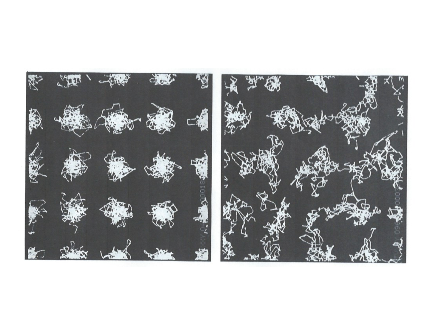
My Father, Edgar Malone Hoover, Junior, taught economics at Harvard ( Ph D 1928 ) and the University of Michigan until World War II brought him to Washington for work with the National Resources Planning Board, the Office of Price Administration, and the Office of Strategic Services. After half a dozen of those years in Washington, followed by a Chemistry major at Oberlin College ( AB 1958 ) I returned to Ann Arbor for a Ph D in Chemical Physics, 1958-1961 . Three of the scientific highlights of those years were [1] a short course in FORTRAN ( a three-hour lecture, taught in a single evening ); [2] George Uhlenbeck’s lectures on Gastheorie, delivered while holding his musty notes at arm’s length; and [3] Andrew De Rocco’s course on statistical mechanics. I was specially inspired by the computer-generated pictures in Berni and Tom Wainwright’s “Molecular Motions”, published in the 1959 Scientific Americanb1 . See Figure 1. When I saw their work I wanted to make some of these manybody dynamics pictures myself.
In the early 1960s the main theoretical route to equations of state was through integral equations for the pair distribution function. This elegant and absorbing approach was soon made thoroughly obsolete by the two simulation techniques of molecular dynamics and Monte Carlo. In 1961-1962 I spent a year in postdoctoral work at Duke with one of John Kirkwood’s students, Jacques Poirier. The result was an improved understanding of integral equations and the Mayers’ virial series. At Duke I shared an office with Jacques’ student, John Nelson Shaw, whose Ph D project was the development of a one-component-plasma Monte Carlo code. Each of the variables in John’s computer program was named for a member of his Family. The code was used soon after by Steve Brush, Harry Sahlin, and Edward Teller at the Livermore Laboratory. Computing was slow in those days. Moore’s 1965 Law was not yet known. Automatic equation-of-state calculations, though soon to be commonplace, were still a few years away in the unforeseeable future.
II Los Alamos and Livermore
When it came time to find a “real job” I was still motivated by the Alder-Wainwright Scientific American article and applied to both Livermore and Los Alamos, where the best computers were. I had interview talks with Bill Wood at Los Alamos and Berni at Livermore. Both places were appealing with rather different physical environments but wonderful opportunities for computational research. The higher salary offer ( though with much shorter vacations ) brought me to Livermore, providing the chance to do real simulations rather than follow the not-so-reliable and not-so-simple integral-equation and virial-series paths.
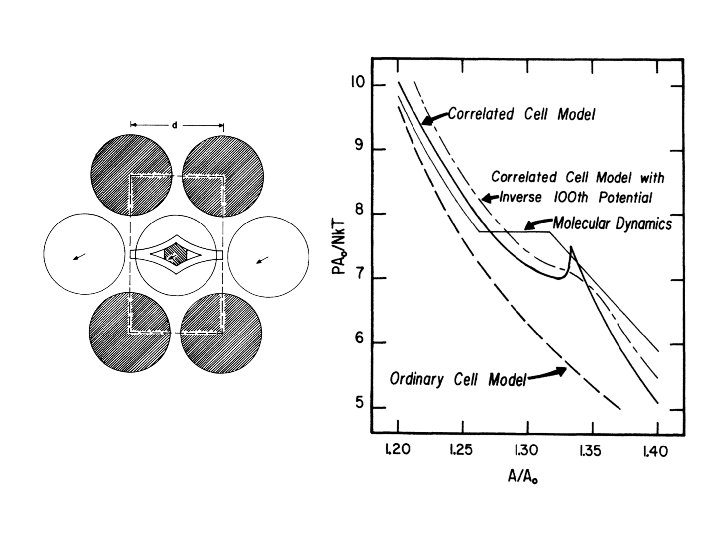
My first California publication, with Berni and Tomb2 , showed that two hard disks, with periodic boundary conditions, give a van der Waals’ pressure-volume loop within a few percent of the large-system transition that had been Berni’s interest ever since his doctoral work with Kirkwood. See Figure 2. Research at Livermore in the early 1960s was a joy, free from the need to apply for grants or to write progress reports. My efforts were strengthened by stimulating collaborations with Francis Ree, Tom Wainwright, and Berni. Often our relatively-long research days were divided up by dinner discussions at Livermore’s Yin Yin restaurant ( 1960 - present ). In those days abalone was still on the menu.
III Work with Francis Ree
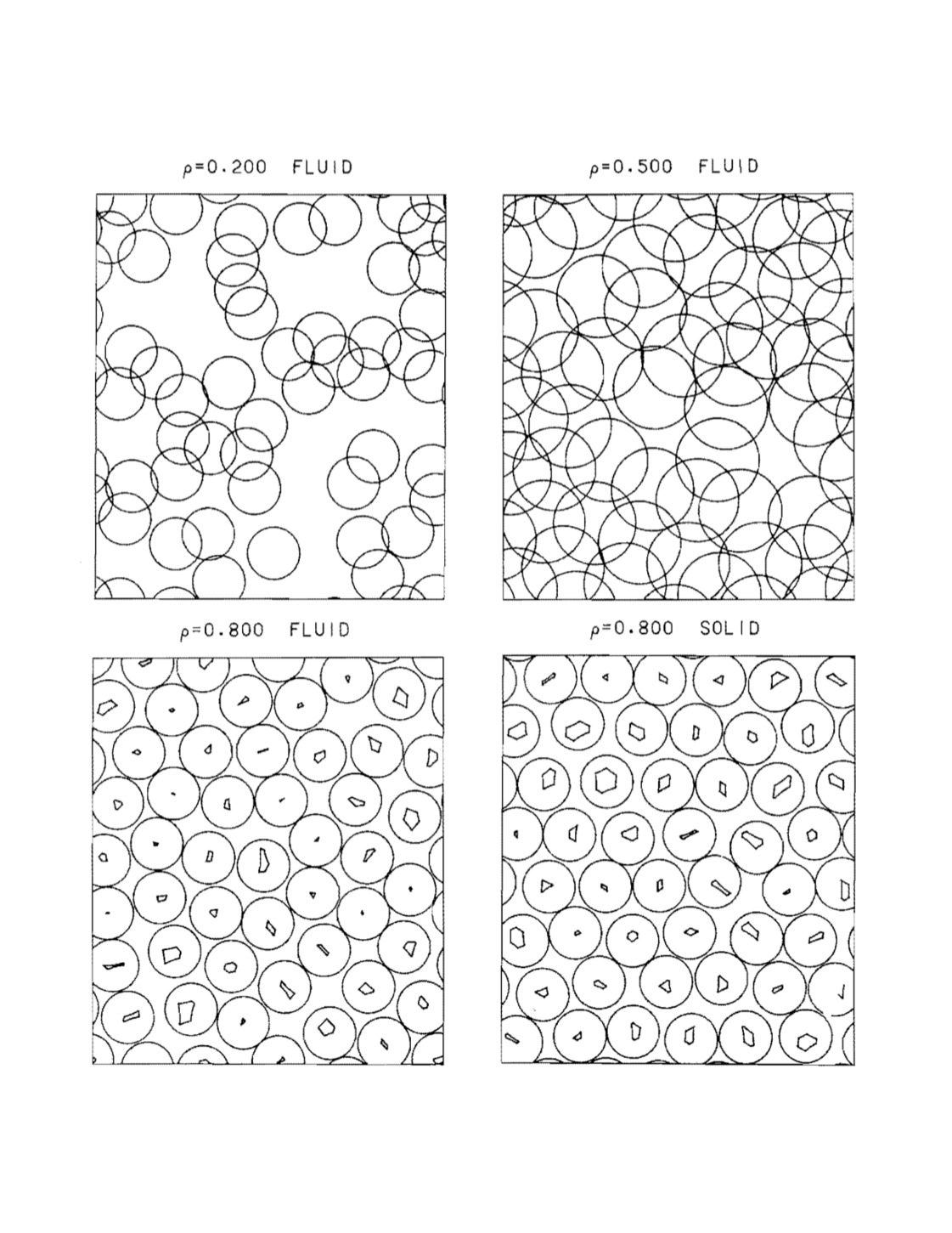
Francis Ree was a student of Henry Eyring’s at the University of Utah, mathematically gifted and a perfect coworker. He and I had the idea to implement Kirkwood’s “communal-entropy” model into Monte Carlo simulations measuring hard-disk and hard-sphere entropies. Kirkwood’s idea was that fluid phases enjoyed an additional shared entropy as a consequence of indistinguishability. This shared entropy was identified with an extra in fluid partition functions. With Edward Teller’s permission to use the considerable computer time entailed Francis and I measured the communal entropy for both disks and spheres. We found that the “extra” fluid entropy varies slowly with density rather than appearing suddenly at melting. We used quantitative measurements to compute precisely the density dependence of the entropy difference between the fluid and solid phases. Our communal-entropy workb3 , along with solid-phase investigations carried out with Berni and David Youngb4 , led to accurate locations of the melting transitions for both disks and spheres.
By the late 1960s Francis and I had had enough virial series and entropy work on the hard-disk and hard-sphere problems. We sought out new directions. Francis enjoyed phase diagram work while I, now working for Russ Duff, pursued nonequilibrium studies. In 1967 I was the very last one of seven authors on a shockwave paper presented by Russ in Parisb5 . This work documented progress toward simulating shockwaves with continuous-potential molecular dynamics. The feasibility of such simulations had been established by Enrico Fermi ( at Los Alamos ), George Vineyard ( at Brookhaven ), as well as Aneesur Rahman ( at Argonne ). I had missed the Fermi and Vineyard work. But Rahman’s later work did get my attentionb6 and I implemented his predictor-corrector algorithm.
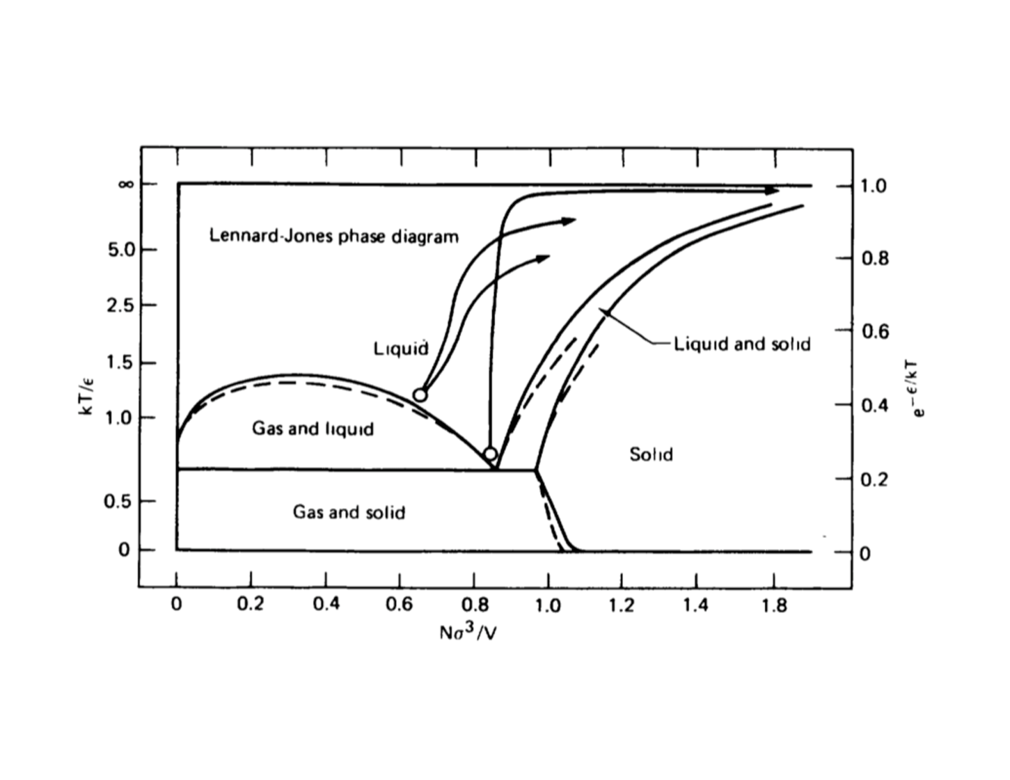
Brad Holian, Bill Moran, Galen Straub, and Ib7 revisited shockwave simulations in the 1980s,
using the much more efficient leapfrog algorithm. That work focused on the strong compression of liquid
states, as is illustrated in Figure 3. Decades later, by then converted to Runge-Kutta, and
working with Paco Uribe and my Wife Carolb8 , we studied more detailed models of the shock process.
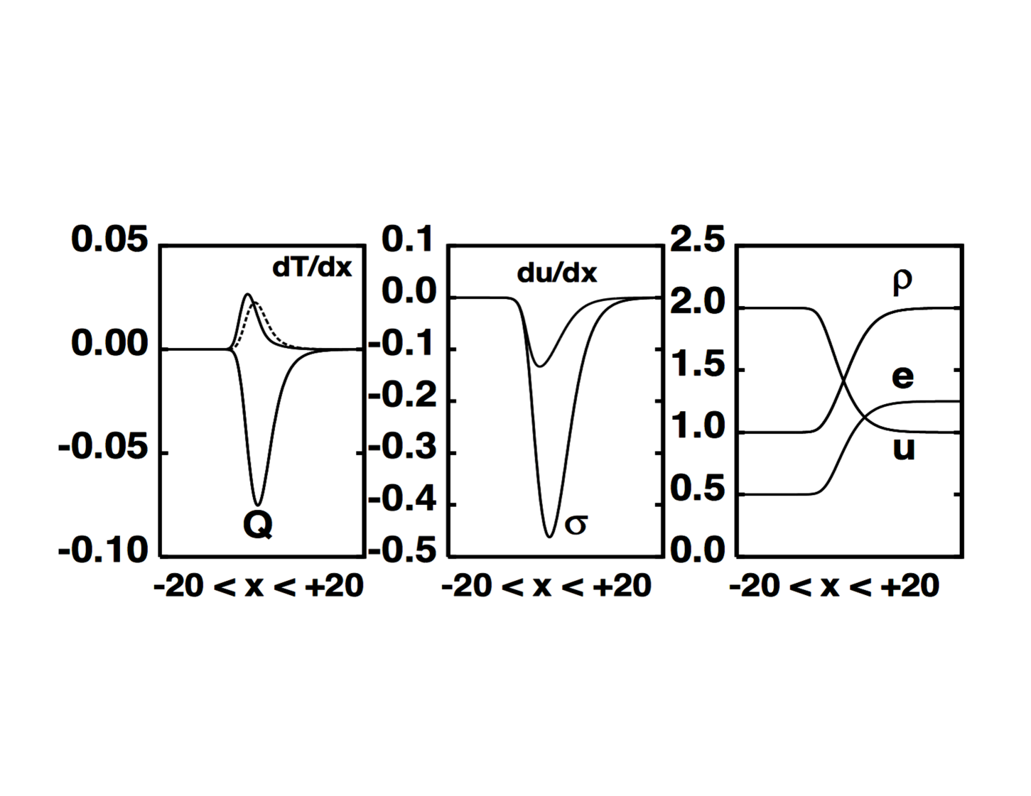
These models included tensor temperature, with . We also found and included
time delays between the fluxes of momentum and energy and the velocity and temperature gradients
driving these fluxes. Figure 4 shows the pressure tensor and the heat-flux vector for a simple model
including these effects. Such a model can describe numerical molecular dynamics data rather
wellb8 .
IV Bill Ashurst and Nonequilibrium Molecular Dynamics
Once several workers (Hans Andersen, John Barker, Frank Canfield, David Chandler, Doug Henderson, Ali Mansoori, Jay Rasaiah, George Stell, and John Weeks) had developed a hard-sphere-based perturbation theory of equilibrium liquid states nonequilibrium simulations opened up as a more promising source of new ideas. In 1971 Berni had helped me into a part-time Professorship at U C Davis through Edward Teller’s Department of Applied Science. My first Ph D student there, Bill Ashurst, from Sandia’s Livermore Laboratory, became interested in modeling shear and heat flows directly, with thermostated “nonequilibrium molecular dynamics”b9 .
Bill used differential feedback to maintain constant boundary velocities and temperatures. Some of his transport coefficients disagreed with those computed from Green-Kubo linear-response theory ( but with factor-of-two errors ) by our French colleagues, Levesque, Verlet, and Kürkijarvib10 . Thanks to a grant from the Academy of Applied Science ( Concord, New Hampshire ), made possible through my U C Davis position, I was able to finance summer research projects with bright high school students. The same grant enabled considerable foreign travel so that I could exchange ideas with the many researchers gathered together in France. Our interests in common with these researchers led to numerous trips to Paris and Orsay to participate in Carl Moser’s simulation workshops. The European contacts were stimulating and pleasant and led to a productive sabbatical in Wien followed up by a thirty-year collaboration with Harald Posch and his colleagues.
Some of the puzzles that arose from this 70s-80s-era work remain today. For example, the effective viscosity measured in a strong shockwave exceeds the small-strainrate Newtonian one by tens of percent. At the same time a steady homogeneous shear flow at the same strain rate exhibits a reduced viscosity, also by tens of percent. These opposite nonlinear effects indicate that there is still much to learn about nonlinear transport.
V Sabbatical Research in Australia, Austria, and Japan
My academic connection to the University of California at Davis made it possible to go on sabbaticals — Canberra ( 1977-1978 ), Wien ( 1985 ), and Yokohama ( 1989-1990 ) . The year in Australia enabled my son Nathan, just graduated from Livermore High, to work with me, exploring another of Berni’s interests, hard-disk and sphere “free volumes”. Kenton Hanson did the three-dimensional work in Berkeley. Nathan and I discovered a percolation transition for hard disks, where the free volume changes from extensive to intensive, at one-fourth of the hard-disk close-packing densityb11 . See Figure 5 . It was interesting to see that solid-phase free volumes are larger than the fluid ones at the same density.
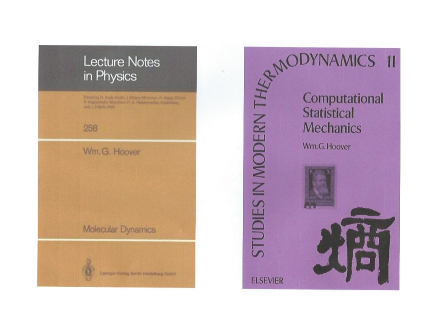
In Wien I worked with Karl Kratky, Harald Posch, and Franz Vesely while lecturing and writing
my first book, “Molecular Dynamics”. The year in Japan, arranged by Shuichi Nosé, was shared
with my new wife Carol, resulting in a longer sequel book, “Computational Statistical
Mechanics” with inspiration and cover art from Shuichi ( Yokohama ) and Harald Posch
( Wien ). See Figure 6 . Nosé’s work changed my outlook on computer simulation. Let us
look at some of the details.
VI Shuichi Nosé and Keio University
During Orwell’s “1984” I came across two amazing papersb12 ; b13 in the Library of Lawrence’s Livermore Laboratory. They were written by a then-unknown Japanese postdoc, Shuichi Nosé, who was working in Canada with Mike Klein. The title of one of Shuichi’s papersb12 describes the gist of his work, “A Molecular Dynamics Method for Simulations in the Canonical Ensemble”. In 1984 this title’s concept seemed to me completely paradoxical. For me “Molecular Dynamics” had generally meant the microcanonical constant-energy ensemble, not the very different constant-temperature canonical one. Although Bill Ashurst and I had long carried out “isokinetic” simulations, for over a decade, the notion of a “canonical” dynamics made no sense to me. I set out to meet Nosé at an upcoming workshop in France and was lucky enough to find him, completely by accident, in Paris’ Orly train station days prior to the workshop’s start.
Nosé’s novel thermostat ideas took me a couple of weeks to digest back then in 1984, even after several hours of conversation before and during the CECAM [ European Center for Atomic and Molecular Calculations ] workshopb14 . Following up Nosé’s new ideas, applied to the harmonic oscillator, revealed a troubling aspect of his new dynamics. The results for long-time averages depended strongly on the initial conditions. A harmonic oscillator, in one dimension and with unit force constant and mass, was the simplest illustration. I could see that his four motion equations, which included a completely novel “time-scaling” variable , its conjugate momentum , and a “number of degrees of freedom” , one for and one for :
could be replaced by an equivalent but simpler and less stiff set of just three equations, with absent and :
Solutions of these three “Nosé-Hoover” equations give trajectories identical to those from the four “Nosé” equations provided that (1) the s match, (2) the initial value of is unity, and (3) the other initial values match: . And it was true, as Nosé had pointed out in his papers, that the three equations were likewise consistent with Gibbs’ canonical distribution, along with an additional Gaussian distribution for the momentum variable :
In fact, by starting with Gibbs’ distribution and working backward using Liouville’s phase-space flow equation, I could obtain Nosé’s “time-scaled” dynamics without any consideration of time scaling at all !
Besides the mysterious time-scaling there was still that troubling fly in the ointment. The thermostated
harmonic-oscillator dynamics doesn’t actually generate all of Gibbs’ distribution. Instead six
percent of its Gaussian measure occupies a “chaotic sea” in which nearby trajectories separate
from one another with a positive exponential growth rate proportional to where
is the system’s largest “Lyapunov exponent”b15 . All of the remaining 94 percent
of the Gaussian distribution is occupied by an infinite set of periodic orbits and their tori. Each such
periodic orbit is surrounded by concentric
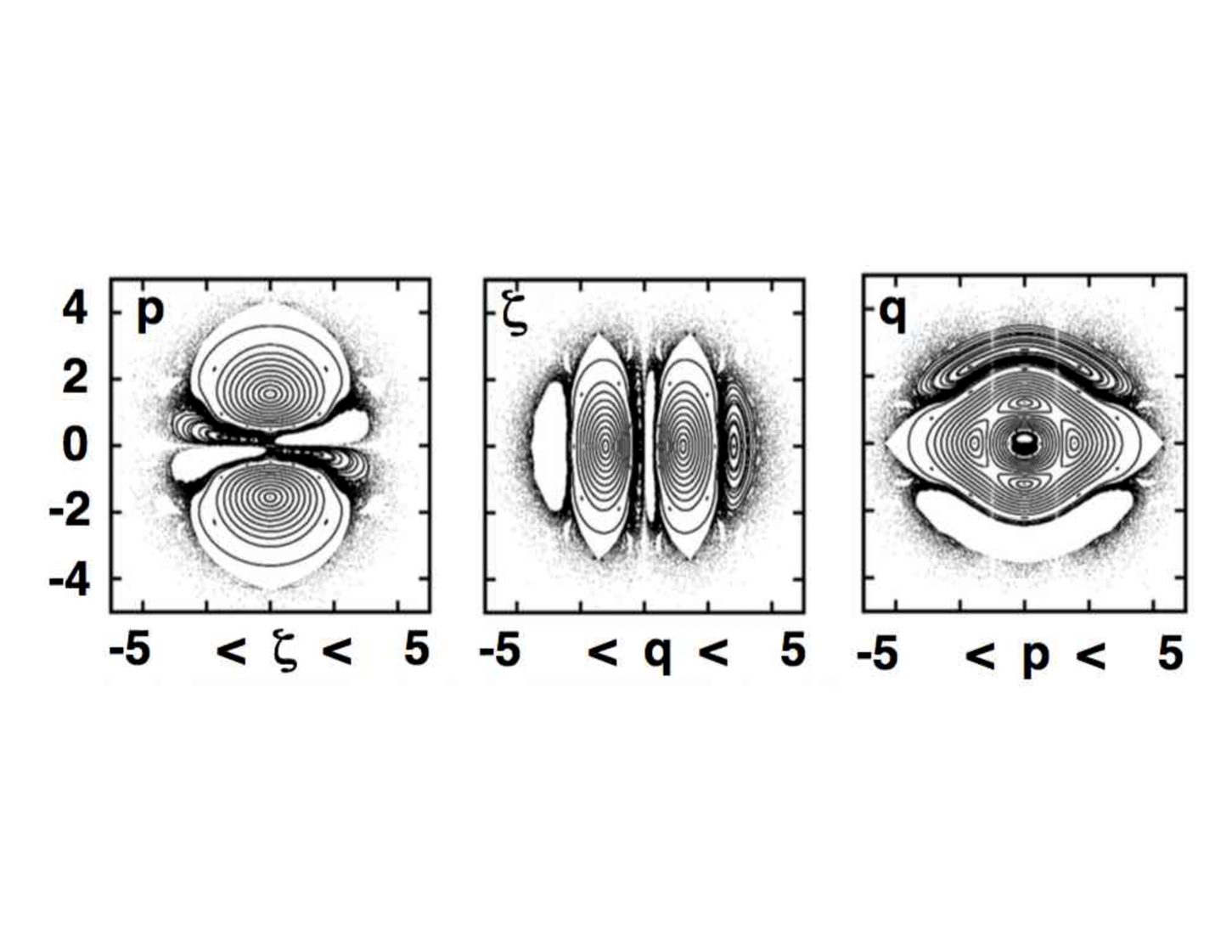
stable toroidal orbits with vanishing Lyapunov exponents, . The complexity of
this distribution can be visualized in the , , and cross sections of
Figure 7. Understanding all of this new information evolved gradually, over a period of years
rather than days.
Ultimately, meeting Shuichi Nosé in Paris in 1984 led me into many new research directions running the gamut from one-body chaos to many-body hydrodynamics, combining ideas from dynamical systems and chaos theory with continuum mechanics and molecular dynamics. In turn this led to a strong and prolific collaboration ( 50 joint papers ) with Harald Posch at Boltzmann’s University on Boltzmanngasse in Wien. By this time I had moved away from Berni’s research interests, which had become mainly quantum mechanical. My own work with Harald and later with Carol involved thermostats and the connections linking continuum mechanics to molecular dynamics and dynamical systems theory.
Many of these projects involved Brad Holian, a gifted student of Berni’s and a real enthusiast for Many-body molecular dynamics. At the other extreme, a single degree of freedom, Brad and I were able to show that the troubling one-dimensional harmonic oscillator, with not only its second velocity moment controlled, but also its fourth, is “ergodic”b16 . That is, with both velocity moments controlled time reversibly, this four-equation model provides all of Gibbs’ canonical distribution for the oscillator as well as Gaussian distributions for the two thermostat variables and :
The idea of formulating a canonical-ensemble dynamics ( giving a Gaussian velocity distribution
defined by its kinetic temperature
rather than constant energy ) was an outgrowth of Shuichi Nosé’s 1984 Magicianshipb12 ; b13 .
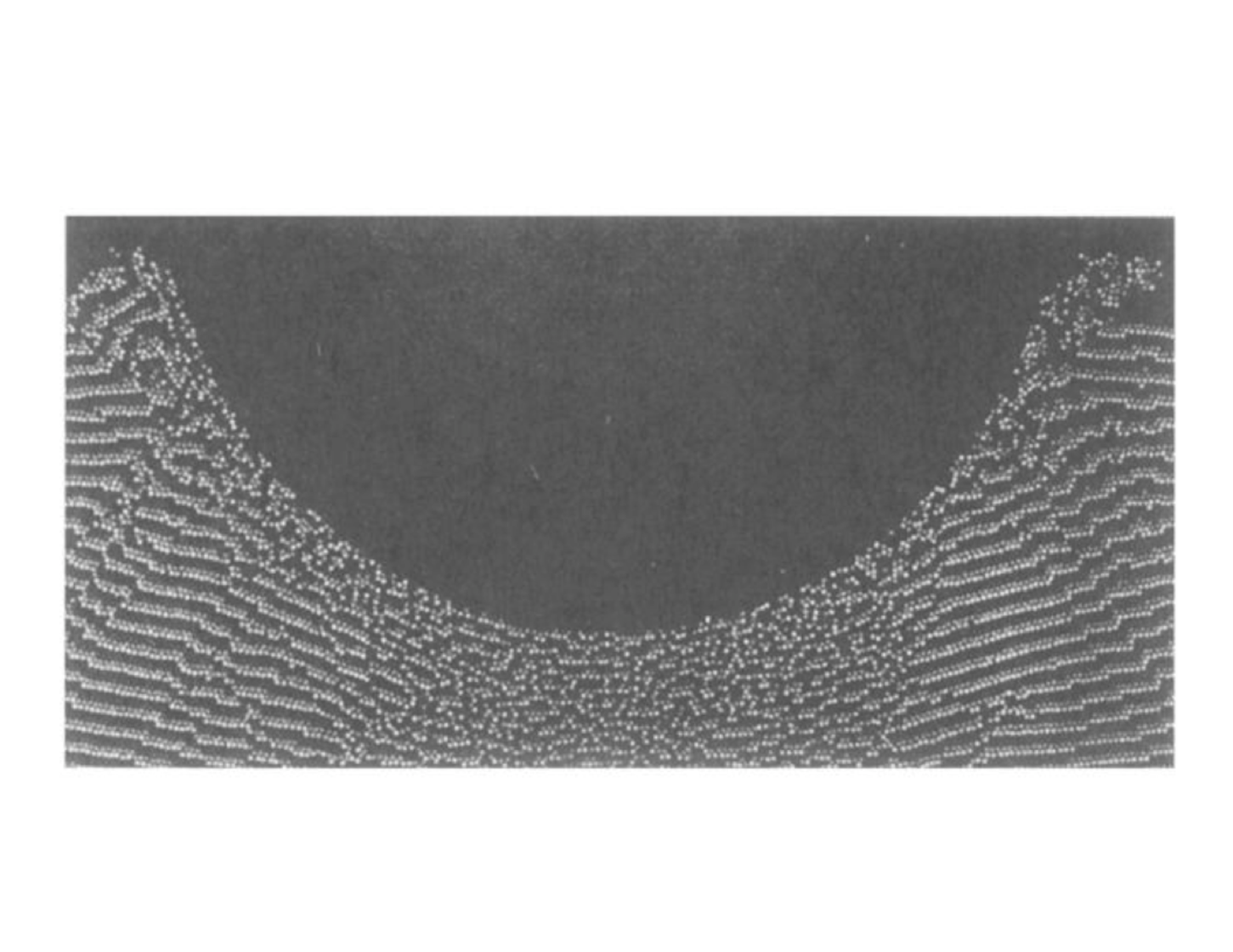
Carol and I had married in 1988 in preparation for a very productive year (1989-1990 ) together at
Nosé’s Keio University. The working conditions in Japan were extremely pleasant, walking to work
at Keio University’s Hiyoshi campus, and with no real duties other than speaking at a few conferences
during the year. We collaborated with Tony De Groot who had built a CRAY-speed computer back at
Livermore with a transputer budget of only $30,000. With many colleagues’ help we were able to
simulate plastic flow with millions of degrees of freedom in reasonable clock times with Tony’s
machine. See Figure 8b17 .
VII Recent Studies of Ergodicity and Lyapunov Instability
During 2014-2015 Carol and I have been enjoying a very fruitful collaboration with Clint Sprott ( Wisconsin ) and Puneet Patra ( a Ph D student of Baidurya Bhattacharya’s in Kharagpur )b18 ; b19 ; b20 . We studied the ergodicity and Lyapunov instability of oscillators exposed to a temperature gradient, . Over the course of a year we came upon several ergodic oscillator models with only three motion equations, rather than four. This was a pleasant surprise. The analysis of three-dimensional topology rather than four- is a tremendous simplification.
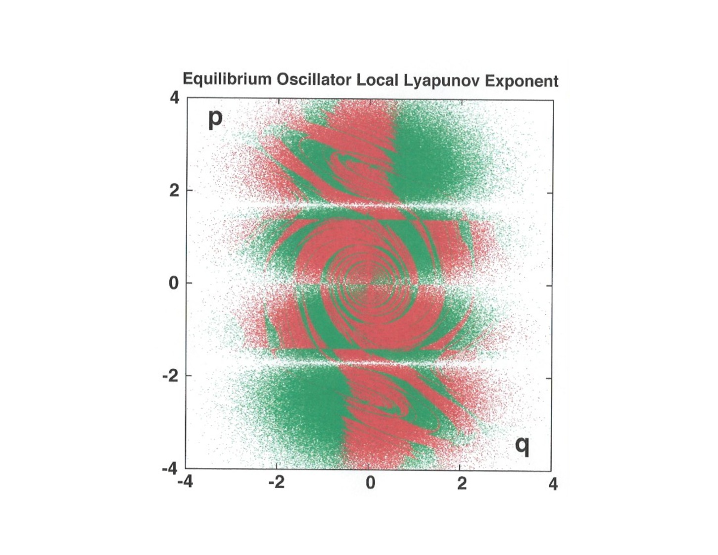
The simplest of all these three-dimensional models incorporates “weak” (integrated) control of both and :
For any initial condition the Gaussian velocity distribution results. And now the chaotic sea embraces the entire three-dimensional phase space.
Figure 9 displays the sign ( red positive and green negative ) of the local Lyapunov exponent just at the moment that the equilibrium trajectory crosses the phase plane . The “local” Lyapunov exponent describes the instantaneous growth or decay rate of a small displacement in the neighborhood of a “reference trajectory”. In the isothermal constant- case an amazing consequence of the three thermostated equations of motion is a simple three-dimensional Gaussian distribution generated by an incredibly-complicated Lyapunov-unstable, but time-reversible, one-dimensional trajectory. Figure 9 conceals a surprise. If a oscillator is viewed in a mirror perpendicular to the axis both and change sign, corresponding to inversion of the cross section through the origin at its center. Diverging trajectories viewed in a mirror likewise diverge. There is also a missing symmetry. One would think that running a trajectory backwards, with unchanged and reversed in sign would replace divergence by convergence so that red in the lower half plane would correspond to green above, and vice versa . This symmetry, though fully consistent with the time-reversible motion equations, is absent. The reason is that the tendency toward divergence or convergence of two trajectories, constrained by a tether, can only depend upon the past, and not the future. This relatively subtle distinction can be clarified by considering the nonequilibrium case where varies with the coordinate . We turn to that case next.
In the nonequilibrium case with temperature – so that the maximum
temperature gradient is – the equations remain time-reversible. Reversing the direction of
time ( as well as the signs of and ) could be expected to reverse the sign of the Lyapunov
exponent. Figures 9 and 10 show that this natural expectation is unwarranted and wrong. The top and
bottom halves of these figures are not simple mirror images. Evidently the time-reversiblity of all
the equations is misleading. Let us consider this observed symmetry breaking in more detail.
VIII Symmetry Breaking in Time-Reversible Flows
From the conceptual standpoint an interesting paradoxical aspect of ( irreversible ) nonequilibrium flows is the time reversibility of their underlying motion equations. This constrast with “real life” motivates Loschmidt’s and Zermélo’s Paradoxes. Loschmidt’s is that forward and backward movies of flows satisfying the irreversible Second Law of Thermodynamics are described by exactly the same time-reversible motion equations in both time directions. Zermélo’s is that any initial phase-space state, no matter how unlikely or odd, will eventually recur due to the bounded nature of the constant-energy phase space. Reversal and recurrence both seem to violate the Second Law.
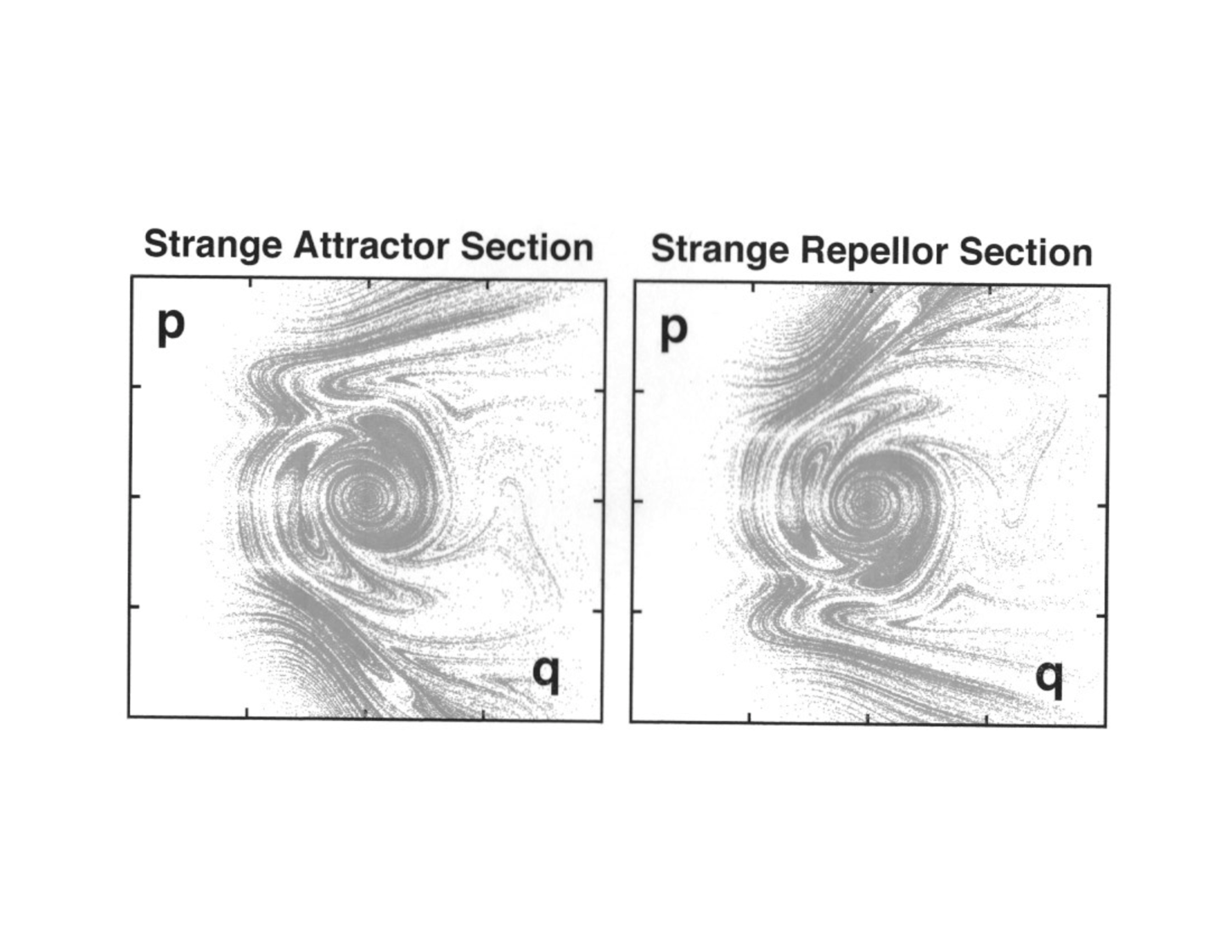
By looking at small nonequilibrium systems [ such as a harmonic oscillator exposed to a temperature gradient, ], we found that the phase-space description of such systems is invariably a unidirectional flow “from” a fractal “repellor” “to” a “strange attractor”. The attractor and repellor correspond to velocity mirror images. The motion forward in time is attractive, with diminishing phase volume, while the reversed expanding motion is repulsive, exponentially unstable, and unobservable. Figure 10 illustrates cross sections of an attractor-repellor pair for the heat conducting oscillator of Section VII with maximum temperature gradient . Neither multifractal object, the attractor nor its mirror-image repellor, with exhibits topological symmetry. Of the 183,264 attractor points shown in the figure 117,364 correspond to positive Lyapunov exponents and 65,900 to negative. It would be worthwhile to carry out detailed comparisons of the Lyapunov exponents both forward and backward in time for such problems.
Thw preponderance of positive local exponents, , is typical of time-reversible chaotic systems either at, or away from, equilibrium. In the nonequilibrium case the smooth Gibbsian phase-space probability density is replaced by the “strange” attractive flow, signalling the loss of phase volume to dissipation. There is a topological symmetry breaking with the two phase-space structures, attractor and repellor, both obeying identical equations of motion, while one has measure zero and the other has all the measure, unity.
The Galton Board problem ( a particle falling at constant kinetic energy through a periodic array of scatterers ) and the conducting oscillator problem ( an oscillator conducting heat in the presence of a temperature gradient ) both furnish three-dimensional models of nonequilibrium steady states. Both provide ergodic fractal geometry, Lyapunov instability, and the symmetry breaking associated with time reversal and with the Second Law of Thermodynamics. This explanation of the Second Law is identical for manybody problems too. My interest in few-body systems was inherited from my earliest work with Berni, dating back to our exploration of one-body cell models for melting as well as our subsequent few-body thermodynamic studies of disks and spheres.
The Lyapunov spectrum ( with all exponents describing the comoving expansion and contraction in an -dimensional space ) characterizes the spatial dependence of instabilities in all of the phase-space directions. It shows that the predominantly negative Lyapunov spectrum describing the condensation of attractive sets onto fractal objects mirrors the predominantly positive spectrum describing the exponentially fast departure of trajectories in the vicinity of the repellor. It is interesting and significant that despite the time-reversibility of the equations of motion the stability of the motions forward and backward is qualitatively different. Just as on a roller coaster or a curvy road the passengers’ motions are sensitive to both the direction of travel and the strange-attractor direction imposed by the Second Law.
Caricatures of these problems, carried out here at Livermore, and at Wien, led to this new understanding of the Second Law of Thermodynamics, first described in a 1987 paper ( submitted twice, with two different titles ! ) with Brad Holian and Harald Poschb21 . In nonequilibrium steady states the motion forward in time has an attractive fractal distribution in phase space with a phase volume of zero. The vanishing volume corresponds to the extreme rarity of the states participating in a steady flow. The time-reversed states, equally rare, make up an inaccessible repellor with a summed-up Lyapunov spectrum which is positive rather than negative. In this way we found that a time-reversible mechanics, based on Nosé’s ideas, provides a clear foundation for irreversible thermodynamics.
IX Conclusion
Berni’s research style, beginning with a simple model confirming a “horseback guess”, followed by painstaking analyses leading to a clear intuitive description of the work and its significance, has led to rapid progress in understanding phase transformations, nonlinear transport, and aspects of dynamical-systems theory. The 2013 Nobel Prizes in Chemistry rewarded Martin Karplus, Michael Levitt, and Arieh Warshel for applications of classical and thermostated molecular dynamics to biomedical problems. Berni has always emphasized the need for simplicity and clarity in his work, with an emphasis on words rather than equations and intuitive arguments rather than formal proofs. After more than a half century of research his way of working seems natural to me and I recognize Berni as a good part of its source. I am looking forward to seeing more of his inspirational work in the years ahead.
X Acknowledgments
My Wife and colleague Carol has helped me throughout. She, Berni, and hundreds of collaborators and colleagues have my Love and Gratitude. I particularly appreciated Brenda Rubenstein’s tireless organizational skills and the staff at the Lawrence Livermore National Laboratory for helping Carol and me to attend and enjoy Berni’s Birthday Symposium.
References
- (1) B. J. Alder and T. E. Wainwright, “Molecular Motions”, Scientific American 201, 113-126 (1959).
- (2) B. J. Alder, W. G. Hoover, and T. E. Wainwright, “Cooperative Motion of Hard Disks Leading to Melting”, Physical Review Letters 11, 241-243 (1963).
- (3) W. G. Hoover and F. H. Ree, “Melting and Communal Entropy for Hard Spheres”, The Journal of Chemical Physics 49, 3609-3617 (1968).
- (4) B. J. Alder, W. G. Hoover, and D. A. Young “Studies in Molecular Dynamics. V. High-Density Equation of State and Entropy for Hard Disks and Spheres”, The Journal of Chemical Physics 49, 3688-3696 (1968).
- (5) R. E. Duff, W. H. Gust, E. B. Royce, M. Ross, A. C. Mitchell, R. N. Keeler, and W. G. Hoover, “Shockwave Studies in Condensed Media”, in Behavior of Dense Media Under High Dynamic Pressures (Gordon and Breach, New York, 1968).
- (6) A. Rahman, “Correlations in the Motion of Atoms in Liquid Argon”, Physical Review A 136, 405-411 (1964).
- (7) B. L. Holian, W. G. Hoover, B. Moran, and G. K. Straub, “Shockwave Structure via Nonequilibrium Molecular Dynamics and Navier-Stokes Continuum Mechanics”, Physical Review A 22, 2798-2808 (1980).
- (8) W. G. Hoover, C. G. Hoover, and F. J. Uribe, “Flexible Macroscopic Models for Dense-Fluid Shockwaves: Partitioning Heat and Work; Delaying Stress and Heat Flux; Two-Temperature Thermal Relaxation”, Proceedings of the International Summer School Conference: “Advanced Problems in Mechanics-2010” organized by the Institute for Problems in Mechanical Engineering of the Russian Academy of Sciences in Mechanics and Engineering under the patronage of the Russian Academy of Sciences = arXiv 1005.1525 (2010).
- (9) W. G. Hoover and W. T. Ashurst, “Nonequilibrium Molecular Dynamics”, Theoretical Chemistry 1 Advances and Perspectives, 1-51 (Academic Press, New York, 1975).
- (10) D. Levesque, L. Verlet, and J. Kürkijarvi, “Computer ‘Experiments’ on Classical Fluids. IV. Transport Properties and Time-Correlation Functions of the Lennard-Jones Liquid Near Its Triple Point”, Physical Review A 7, 1690-1700 (1973). Note their Acknowledgment for “many interesting and stimulating discussions with Professor B. J. Alder”.
- (11) W. G. Hoover, N. E. Hoover, and K. Hanson, “Exact Hard-Disk Free Volumes”, The Journal of Chemical Physics 70, 1837-1844 (1979).
- (12) S. Nosé, “A Molecular Dynamics Method for Simulations in the Canonical Ensemble”, Molecular Physics 52, 255-268 (1984).
- (13) S. Nosé, “A Unified Formulation of the Constant Temperature Molecular Dynamics Methods”, The Journal of Chemical Physics 81, 511-519 (1984).
- (14) W. G. Hoover, “Canonical Dynamics: Equilibrium Phase-Space Distributions”, Physical Review A 31, 1695-1697 (1985).
- (15) W. G. Hoover, C. G. Hoover, and J. C. Sprott, “Nonequilibrium Systems : Hard Disks and Harmonic Oscillators Near and Far From Equilibrium”, Molecular Simulation (in press, 2015) = arXiv 1507.08302.
- (16) W. G. Hoover and B. L. Holian, “Kinetic Moments Method for the Canonical Ensemble Distribution”, Physics Letters A 211, 253-257 (1996).
- (17) W. G. Hoover, A. J. De Groot, C. G. Hoover, I. F. Stowers, T. Kawai, B. L. Holian, T. Boku, S. Ihara, and J. Belak, “Large-Scale Elastic-Plastic Indentation Simulations via Molecular Dynamics”, Physical Review A 42, 5844-5853 (1990).
- (18) W. G. Hoover, J. C. Sprott, and P. K. Patra, “Deterministic Time-Reversible Thermostats : Chaos, Ergodicity, and the Zeroth Law of Thermodynamics”, Molecular Physics (in press, 2015) = arXiv 1501.03875.
- (19) W. G. Hoover, J. C. Sprott, and P. K. Patra, “Ergodic Time-Reversible Chaos for Gibbs’ Canonical Oscillator”, Physics Letters A (in press, 2015) = arXiv 1503.06749.
- (20) W. G. Hoover, J. C. Sprott, and C. G. Hoover, “Ergodicity of a Singly-Thermostated Harmonic Oscillator”, Communications in Nonlinear Science and Numerical Simulation 32, 234-240 (2016) = arXiv 1504.07654.
- (21) B. L. Holian, W. G. Hoover, and H. A. Posch, “Second-Law Irreversibility of Reversible Mechanical Systems” = “Resolution of Loschmidt’s Paradox: the Origin of Irreversible Behavior in Reversible Atomistic Dynamics”, Physical Review Letters 59, 10-13 (1987) .