An Asynchronous Parallel Stochastic Coordinate Descent Algorithm

Consider the convex optimization problem

where $\Omega\subset\mathbb{R}^{n}$ is a closed convex set and $f$ is a smooth convex mapping from an open neighborhood of $\Omega$ to $\mathbb{R}$. We consider two particular cases of $\Omega$ in this paper: the unconstrained case $\Omega=\mathbb{R}^{n}$, and the separable case

where each $\Omega_{i}$, $i=1,2,\dotsc,n$ is a closed subinterval of the real line.

Formulations of the type (1,2) arise in many data analysis and machine learning problems, for example, support vector machines (linear or nonlinear dual formulation) (Cortes and Vapnik, 1995), LASSO (after decomposing $x$ into positive and negative parts) (Tibshirani, 1996), and logistic regression. Algorithms based on gradient and approximate or partial gradient information have proved effective in these settings. We mention in particular gradient projection and its accelerated variants (Nesterov, 2004), accelerated proximal gradient methods for regularized objectives (Beck and Teboulle, 2009), and stochastic gradient methods (Nemirovski et al., 2009; Shamir and Zhang, 2013). These methods are inherently serial, in that each iteration depends on the result of the previous iteration. Recently, parallel multicore versions of stochastic gradient and stochastic coordinate descent have been described for problems involving large data sets; see for example Niu et al. (2011); Richtárik and Takáč (2012b); Avron et al. (2014).

This paper proposes an asynchronous stochastic coordinate descent (AsySCD) algorithm for convex optimization. Each step of AsySCD chooses an index $i\in\{1,2,\dotsc,n\}$ and subtracts a short, constant, positive multiple of the $i$th partial gradient $\nabla_{i}f(x):=\partial f/\partial x_{i}$ from the $i$th component of $x$. When separable constraints (2) are present, the update is “clipped” to maintain feasibility with respect to $\Omega_{i}$. Updates take place in parallel across the cores of a multicore system, without any attempt to synchronize computation between cores. We assume that there is a bound $\tau$ on the age of the updates, that is, no more than $\tau$ updates to $x$ occur between the time at which a processor reads $x$ (and uses it to evaluate one element of the gradient) and the time at which this processor makes its update to a single element of $x$. (A similar model of parallel asynchronous computation was used in Hogwild! (Niu et al., 2011).) Our implementation, described in Section 6, is a little more complex than this simple model would suggest, as it is tailored to the architecture of the Intel Xeon machine that we use for experiments.

We show that linear convergence can be attained if an “essential strong convexity” property (3) holds, while sublinear convergence at a “$1/K$” rate can be proved for general convex functions. Our analysis also defines a sufficient condition for near-linear speedup in the number of cores used. This condition relates the value of delay parameter $\tau$ (which relates to the number of cores / threads used in the computation) to the problem dimension $n$. A parameter that quantifies the cross-coordinate interactions in $\nabla f$ also appears in this relationship. When the Hessian of $f$ is nearly diagonal, the minimization problem can almost be separated along the coordinate axes, so higher degrees of parallelism are possible.

We review related work in Section 2. Section 3 specifies the proposed algorithm. Convergence results for unconstrained and constrained cases are described in Sections 4 and 5, respectively, with proofs given in the appendix. Computational experience is reported in Section 6. We discuss several variants of AsySCD in Section 7. Some conclusions are given in Section 8.

This section reviews some related work on coordinate relaxation and stochastic gradient algorithms.

Among cyclic coordinate descent algorithms, Tseng (2001) proved the convergence of a block coordinate descent method for nondifferentiable functions with certain conditions. Local and global linear convergence were established under additional assumptions, by Luo and Tseng (1992) and Wang and Lin (2014), respectively. Global linear (sublinear) convergence rate for strongly (weakly) convex optimization was proved by Beck and Tetruashvili (2013). Block-coordinate approaches based on proximal-linear subproblems are described by Tseng and Yun (2009, 2010). Wright (2012) uses acceleration on reduced spaces (corresponding to the optimal manifold) to improve the local convergence properties of this approach.

Stochastic coordinate descent is almost identical to cyclic coordinate descent except selecting coordinates in a random manner. Nesterov (2012) studied the convergence rate for a stochastic block coordinate descent method for unconstrained and separably constrained convex smooth optimization, proving linear convergence for the strongly convex case and a sublinear $1/K$ rate for the convex case. Extensions to minimization of composite functions are described by Richtárik and Takáč (2012a) and Lu and Xiao (2013).

Synchronous parallel methods distribute the workload and data among multiple processors, and coordinate the computation among processors. Ferris and Mangasarian (1994) proposed to distribute variables among multiple processors and optimize concurrently over each subset. The synchronization step searches the affine hull formed by the current iterate and the points found by each processor. Similar ideas appeared in (Mangasarian, 1995), with a different synchronization step. Goldfarb and Ma (2012) considered a multiple splitting algorithm for functions of the form $f(x)=\sum_{k=1}^{N}f_{k}(x)$ in which $N$ models are optimized separately and concurrently, then combined in an synchronization step. The alternating direction method-of-multiplier (ADMM) framework (Boyd et al., 2011) can also be implemented in parallel. This approach dissects the problem into multiple subproblems (possibly after replication of primal variables) and optimizes concurrently, then synchronizes to update multiplier estimates. Duchi et al. (2012) described a subgradient dual-averaging algorithm for partially separable objectives, with subgradient evaluations distributed between cores and combined in ways that reflect the structure of the objective. Parallel stochastic gradient approaches have received broad attention; see Agarwal and Duchi (2011) for an approach that allows delays between evaluation and update, and Cotter et al. (2011) for a minibatch stochastic gradient approach with Nesterov acceleration. Shalev-Shwartz and Zhang (2013) proposed an accelerated stochastic dual coordinate ascent method.

Among synchronous parallel methods for (block) coordinate descent, Richtárik and Takáč (2012b) described a method of this type for convex composite optimization problems. All processors update randomly selected coordinates or blocks, concurrently and synchronously, at each iteration. Speedup depends on the sparsity of the data matrix that defines the loss functions. Several variants that select blocks greedily are considered by Scherrer et al. (2012) and Peng et al. (2013). Yang (2013) studied the parallel stochastic dual coordinate ascent method and emphasized the balance between computation and communication.

We turn now to asynchronous parallel methods. Bertsekas and Tsitsiklis (1989) introduced an asynchronous parallel implementation for general fixed point problems $x=q(x)$ over a separable convex closed feasible region. (The optimization problem (1) can be formulated in this way by defining $q(x):=\mathcal{P}_{\Omega}[(I-\alpha\nabla f)(x)]$ for some fixed $\alpha>0$.) Their analysis allows inconsistent reads for $x$, that is, the coordinates of the read $x$ have different “ages.” Linear convergence is established if all ages are bounded and $\nabla^{2}f(x)$ satisfies a diagonal dominance condition guaranteeing that the iteration $x=q(x)$ is a maximum-norm contraction mapping for sufficient small $\alpha$. However, this condition is strong — stronger, in fact, than the strong convexity condition. For convex quadratic optimization $f(x)={1\over 2}x^{T}Ax+bx$, the contraction condition requires diagonal dominance of the Hessian: $A_{ii}>\sum_{i\neq j}|A_{ij}|$ for all $i=1,2,\dotsc,n$. By comparison, AsySCD guarantees linear convergence rate under the essential strong convexity condition (3), though we do not allow inconsistent read. (We require the vector $x$ used for each evaluation of $\nabla_{i}f(x)$ to have existed at a certain point in time.)

Hogwild! (Niu et al., 2011) is a lock-free, asynchronous parallel implementation of a stochastic-gradient method, targeted to a multicore computational model similar to the one considered here. Its analysis assumes consistent reading of $x$, and it is implemented without locking or coordination between processors. Under certain conditions, convergence of Hogwild! approximately matches the sublinear $1/K$ rate of its serial counterpart, which is the constant-steplength stochastic gradient method analyzed in Nemirovski et al. (2009).

We also note recent work by Avron et al. (2014), who proposed an asynchronous linear solver to solve $Ax=b$ where $A$ is a symmetric positive definite matrix, proving a linear convergence rate. Both inconsistent- and consistent-read cases are analyzed in this paper, with the convergence result for inconsistent read being slightly weaker.

The AsySCD algorithm described in this paper was extended to solve the composite objective function consisting of a smooth convex function plus a separable convex function in a later work (Liu and Wright, 2014), which pays particular attention to the inconsistent-read case.

In AsySCD, multiple processors have access to a shared data structure for the vector $x$, and each processor is able to compute a randomly chosen element of the gradient vector $\nabla f(x)$. Each processor repeatedly runs the following coordinate descent process (the steplength parameter $\gamma$ is discussed further in the next section):

• R:

  Choose an index $i\in\{1,2,\dotsc,n\}$ at random, read $x$, and evaluate $\nabla_{i}f(x)$;

• U:

  Update component $i$ of the shared $x$ by taking a step of length $\gamma/L_{\max}$ in the direction $-\nabla_{i}f(x)$.

Since these processors are being run concurrently and without synchronization, $x$ may change between the time at which it is read (in step R) and the time at which it is updated (step U). We capture the system-wide behavior of AsySCD in Algorithm 1. There is a global counter $j$ for the total number of updates; $x_{j}$ denotes the state of $x$ after $j$ updates. The index $i(j)\in\{1,2,\dotsc,n\}$ denotes the component updated at step $j$. $k(j)$ denotes the $x$-iterate at which the update applied at iteration $j$ was calculated. Obviously, we have $k(j)\leq j$, but we assume that the delay between the time of evaluation and updating is bounded uniformly by a positive integer $\tau$, that is, $j-k(j)\leq\tau$ for all $j$. The value of $\tau$ captures the essential parallelism in the method, as it indicates the number of processors that are involved in the computation.

The projection operation $P_{\Omega}$ onto the feasible set is not needed in the case of unconstrained optimization. For separable constraints (2), it requires a simple clipping operation on the $i(j)$ component of $x$.

We note several differences with earlier asynchronous approaches. Unlike the asynchronous scheme in Bertsekas and Tsitsiklis (1989, Section 6.1), the latest value of $x$ is updated at each step, not an earlier iterate. Although our model of computation is similar to Hogwild! (Niu et al., 2011), the algorithm differs in that each iteration of AsySCD evaluates a single component of the gradient exactly, while Hogwild!  computes only a (usually crude) estimate of the full gradient. Our analysis of AsySCD below is comprehensively different from that of Niu et al. (2011), and we obtain stronger convergence results.

This section presents results about convergence of AsySCD in the unconstrained case $\Omega=\mathbb{R}^{n}$. The theorem encompasses both the linear rate for essentially strongly convex $f$ and the sublinear rate for general convex $f$. The result depends strongly on the delay parameter $\tau$. (Proofs of results in this section appear in Appendix A.) In Algorithm 1, the indices $i(j)$, $j=0,1,2,\dotsc$ are random variables. We denote the expectation over all random variables as $\mathbb{E}$, the conditional expectation in term of $i(j)$ given $i(0),i(1),\cdots,i(j-1)$ as $\mathbb{E}_{i(j)}$.

A crucial issue in AsySCD is the choice of steplength parameter $\gamma$. This choice involves a tradeoff: We would like $\gamma$ to be long enough that significant progress is made at each step, but not so long that the gradient information computed at step $k(j)$ is stale and irrelevant by the time the update is applied at step $j$. We enforce this tradeoff by means of a bound on the ratio of expected squared norms on $\nabla f$ at successive iterates; specifically,

where $\rho>1$ is a user defined parameter. The analysis becomes a delicate balancing act in the choice of $\rho$ and steplength $\gamma$ between aggression and excessive conservatism. We find, however, that these values can be chosen to ensure steady convergence for the asynchronous method at a linear rate, with rate constants that are almost consistent with vanilla short-step full-gradient descent.

We use the following assumption in some of the results of this section.

Note that this assumption is not needed in our convergence results in the case of strongly convex functions. in our theorems below, it is invoked only when considering general convex functions.

This theorem demonstrates linear convergence (9) for AsySCD in the unconstrained essentially strongly convex case. This result is better than that obtained for Hogwild! (Niu et al., 2011), which guarantees only sublinear convergence under the stronger assumption of strict convexity.

The following corollary proposes an interesting particular choice of the parameters for which the convergence expressions become more comprehensible. The result requires a condition on the delay bound $\tau$ in terms of $n$ and the ratio $L_{\max}/L_{\mbox{\rm\scriptsize res}}$.

We note that the linear rate (13) is broadly consistent with the linear rate for the classical steepest descent method applied to strongly convex functions, which has a rate constant of $(1-2l/L)$, where $L$ is the standard Lipschitz constant for $\nabla f$. If we assume (not unreasonably) that $n$ steps of stochastic coordinate descent cost roughly the same as one step of steepest descent, and note from (13) that $n$ steps of stochastic coordinate descent would achieve a reduction factor of about $(1-l/(2L_{\max}))$, a standard argument would suggest that stochastic coordinate descent would require about $4L_{\max}/L$ times more computation. (Note that $L_{\max}/L\in[1/n,1]$.) The stochastic approach may gain an advantage from the parallel implementation, however. Steepest descent requires synchronization and careful division of gradient evaluations, whereas the stochastic approach can be implemented in an asynchronous fashion.

For the general convex case, (14) defines a sublinear rate, whose relationship with the rate of the steepest descent for general convex optimization is similar to the previous paragraph.

As noted in Section 1, the parameter $\tau$ is closely related to the number of cores that can be involved in the computation, without degrading the convergence performance of the algorithm. In other words, if the number of cores is small enough such that (11) holds, the convergence expressions (13), (14) do not depend on the number of cores, implying that linear speedup can be expected. A small value for the ratio $L_{\mbox{\rm\scriptsize res}}/L_{\max}$ (not much greater than $1$) implies a greater degree of potential parallelism. As we note at the end of Section 1, this ratio tends to be small in some important applications — a situation that would allow $O(\sqrt{n})$ cores to be used with near-linear speedup.

We conclude this section with a high-probability estimate for convergence of the sequence of function values.

This section considers the case of separable constraints (2). We show results about convergence rates and high-probability complexity estimates, analogous to those of the previous section. Proofs appear in Appendix B.

As in the unconstrained case, the steplength $\gamma$ should be chosen to ensure steady progress while ensuring that update information does not become too stale. Because constraints are present, the ratio (5) is no longer appropriate. We use instead a ratio of squares of expected differences in successive primal iterates:

where $\bar{x}_{j+1}$ is the hypothesized full update obtained by applying the single-component update to every component of $x_{j}$, that is,

In the unconstrained case $\Omega=\mathbb{R}^{n}$, the ratio (18) reduces to

which is evidently related to (5), but not identical.

We have the following result concerning convergence of the expected error to zero.

Similarly to the unconstrained case, the following corollary proposes an interesting particular choice for the parameters for which the convergence expressions become more comprehensible. The result requires a condition on the delay bound $\tau$ in terms of $n$ and the ratio $L_{\max}/L_{\mbox{\rm\scriptsize res}}$.

Similarly to Section 4, and provided $\tau$ satisfies (25), the convergence rate is not affected appreciably by the delay bound $\tau$, and near-linear speedup can be expected for multicore implementations when (25) holds. This condition is more restrictive than (11) in the unconstrained case, but still holds in many problems for interesting values of $\tau$. When $L_{\mbox{\rm\scriptsize res}}/L_{\max}$ is bounded independently of dimension, the maximal number of cores allowed is of the the order of $n^{1/4}$, which is smaller than the $O(n^{1/2})$ value obtained for the unconstrained case.

We conclude this section with another high-probability bound, whose proof tracks that of Theorem 3.

We illustrate the behavior of two variants of the stochastic coordinate descent approach on test problems constructed from several data sets. Our interests are in the efficiency of multicore implementations (by comparison with a single-threaded implementation) and in performance relative to alternative solvers for the same problems.

All our test problems have the form (1), with either $\Omega=\mathbb{R}^{n}$ or $\Omega$ separable as in (2). The objective $f$ is quadratic, that is,

with $Q$ symmetric positive definite.

Our implementation of AsySCD is called DIMM-WITTED (or DW for short). It runs on various numbers of threads, from 1 to 40, each thread assigned to a single core in our 40-core Intel Xeon architecture. Cores on the Xeon architecture are arranged into four sockets — ten cores per socket, with each socket having its own memory. Non-uniform memory access (NUMA) means that memory accesses to local memory (on the same socket as the core) are less expensive than accesses to memory on another socket. In our DW implementation, we assign each socket an equal-sized “slice” of $Q$, a row submatrix. The components of $x$ are partitioned between cores, each core being responsible for updating its own partition of $x$ (though it can read the components of $x$ from other cores). The components of $x$ assigned to the cores correspond to the rows of $Q$ assigned to that core’s socket. Computation is grouped into “epochs,” where an epoch is defined to be the period of computation during which each component of $x$ is updated exactly once. We use the parameter $p$ to denote the number of epochs that are executed between reordering (shuffling) of the coordinates of $x$. We investigate both shuffling after every epoch ($p=1$) and after every tenth epoch ($p=10$). Access to $x$ is lock-free, and updates are performed asynchronously. This update scheme does not implement exactly the “sampling with replacement” scheme analyzed in previous sections, but can be viewed as a high performance, practical adaptation of the AsySCD method.

To do each coordinate descent update, a thread must read the latest value of $x$. Most components are already in the cache for that core, so that it only needs to fetch those components recently changed. When a thread writes to $x_{i}$, the hardware ensures that this $x_{i}$ is simultaneously removed from other cores, signaling that they must fetch the updated version before proceeding with their respective computations.

Although DW is not a precise implementation of AsySCD, it largely achieves the consistent-read condition that is assumed by the analysis. Inconsistent read happens on a core only if the following three conditions are satisfied simultaneously:

• •

  A core does not finish reading recently changed coordinates of $x$ (note that it needs to read no more than $\tau$ coordinates);

• •

  Among these recently changed coordinates, modifications take place both to coordinates that have been read and that are still to be read by this core;

• •

  Modification of the already-read coordinates happens earlier than the modification of the still-unread coordinates.

Inconsistent read will occur only if at least two coordinates of $x$ are modified twice during a stretch of approximately $\tau$ updates to $x$ (that is, iterations of Algorithm 1). For the DW implementation, inconsistent read would require repeated updating of a particular component in a stretch of approximately $\tau$ iterations that straddles two epochs. This event would be rare, for typical values of $n$ and $\tau$. Of course, one can avoid the inconsistent read issue altogether by changing the shuffling rule slightly, enforcing the requirement that no coordinate can be modified twice in a span of $\tau$ iterations. From the practical perspective, this change does not improve performance, and detracts from the simplicity of the approach. From the theoretical perspective, however, the analysis for the inconsistent-read model would be interesting and meaningful, and we plan to study this topic in future work.

The first test problem QP is an unconstrained, regularized least squares problem constructed with synthetic data. It has the form

All elements of $A\in\mathbb{R}^{m\times n}$, the true model $\tilde{x}\in\mathbb{R}^{n}$, and the observation noise vector $\delta\in\mathbb{R}^{m}$ are generated in i.i.d. fashion from the Gaussian distribution $\mathcal{N}(0,1)$, following which each column in $A$ is scaled to have a Euclidean norm of $1$. The observation $b\in\mathbb{R}^{m}$ is constructed from $A\tilde{x}+\delta\|A\tilde{x}\|/(5m)$. We choose $m=6000$, $n=20000$, and $\alpha=0.5$. We therefore have $L_{\max}=1+\alpha=1.5$ and

With this estimate, the condition (11) is satisfied when delay parameter $\tau$ is less than about $95$. In Algorithm 1, we set the steplength parameter $\gamma$ to $1$, and we choose initial iterate to be $x_{0}=\mathbb{0}$. We measure convergence of the residual norm $\|\nabla f(x)\|$.

Our second problem QPc is a bound-constrained version of (29):

The methodology for generating $A$ and $\tilde{x}$ and for choosing the values of $m$, $n$, $\gamma$, and $x_{0}$ is the same as for (29). We measure convergence via the residual $\|x-\mathcal{P}_{\Omega}(x-\nabla f(x))\|$, where $\Omega$ is the nonnegative orthant $\mathbb{R}^{n}_{+}$. At the solution of (30), about half the components of $x$ are at their lower bound of $0$.

Our third and fourth problems are quadratic penalty functions for linear programming relaxations of vertex cover problems on large graphs. The vertex cover problem for an undirected graph with edge set $E$ and vertex set $V$ can be written as a binary linear program:

By relaxing each binary constraint to the interval $[0,1]$, introducing slack variables for the cover inequalities, we obtain a problem of the form

This has the form

for $n=|V|+|E|$. The test problem (31) is a regularized quadratic penalty reformulation of this linear program for some penalty parameter $\beta$:

with $\beta=5$. Two test data sets Amazon and DBLP have dimensions $n=561050$ and $n=520891$, respectively.

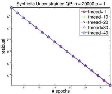
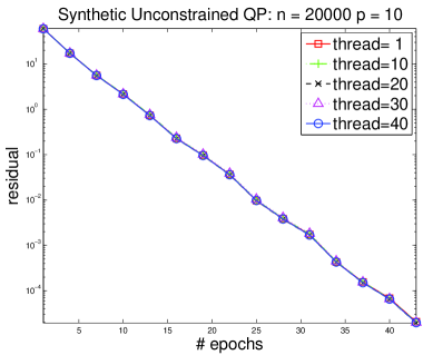
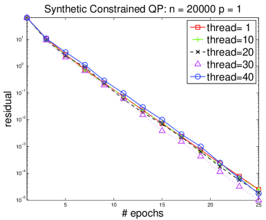
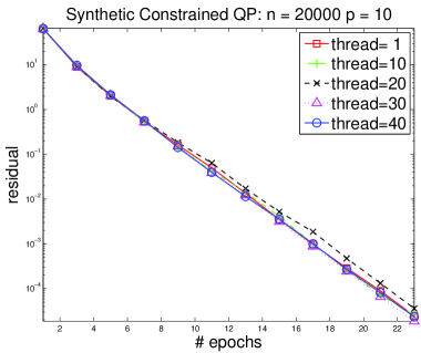
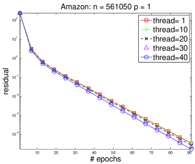
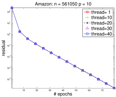
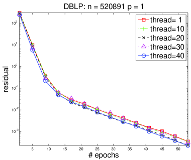
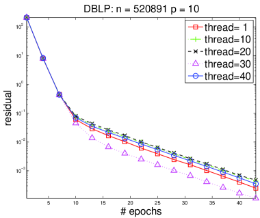
We tracked the behavior of the residual as a function of the number of epochs, when executed on different numbers of cores. Figure 1 shows convergence behavior for each of our four test problems on various numbers of cores with two different shuffling periods: $p=1$ and $p=10$. We note the following points.

• •

  The total amount of computation to achieve any level of precision appears to be almost independent of the number of cores, at least up to 40 cores. In this respect, the performance of the algorithm does not change appreciably as the number of cores is increased. Thus, any deviation from linear speedup is due not to degradation of convergence speed in the algorithm but rather to systems issues in the implementation.

• •

  When we reshuffle after every epoch ($p=1$), convergence is slightly faster in synthetic unconstrained QP but slightly slower in Amazon and DBLP than when we do occasional reshuffling ($p=10$). Overall, the convergence rates with different shuffling periods are comparable in the sense of epochs. However, when the dimension of the variable is large, the shuffling operation becomes expensive, so we would recommend using a large value for $p$ for large-dimensional problems.

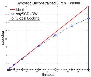
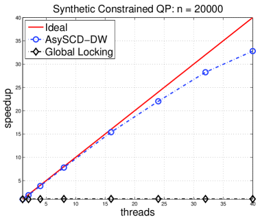
Results for speedup on multicore implementations are shown in Figures 2 and 3 for DW with $p=10$. Speedup is defined as follows:

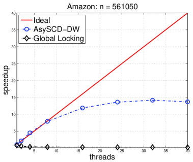
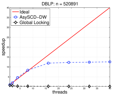
Near-linear speedup can be observed for the two QP problems with synthetic data. For Problems 3 and 4, speedup is at most 12-14; there are few gains when the number of cores exceeds about 12. We believe that the degradation is due mostly to memory contention. Although these problems have high dimension, the matrix $Q$ is very sparse (in contrast to the dense $Q$ for the synthetic data set). Thus, the ratio of computation to data movement / memory access is much lower for these problems, making memory contention effects more significant.

Figures 2 and 3 also show results of a global-locking strategy for the parallel stochastic coordinate descent method, in which the vector $x$ is locked by a core whenever it performs a read or update. The performance curve for this strategy hugs the horizontal axis; it is not competitive.

Wall clock times required for the four test problems on $1$ and $40$ cores, to reduce residuals below $10^{-5}$ are shown in Table 1. (Similar speedups are noted when we use a convergence tolerance looser than $10^{-5}$.)

All problems reported on above are essentially strongly convex. Similar speedup properties can be obtained in the weakly convex case as well. We show speedups for the QPc problem with $\alpha=0$. Table 2 demonstrates similar speedup to the essentially strongly convex case shown in Figure 2.

Turning now to comparisons between AsySCD and alternative algorithms, we start by considering the basic gradient descent method. We implement gradient descent in a parallel, synchronous fashion, distributing the gradient computation load on multiple cores and updating the variable $x$ in parallel at each step. The resulting implementation is called SynGD. Table 3 reports running time and speedup of both AsySCD over SynGD, showing a clear advantage for AsySCD. A high price is paid for the synchronization requirement in SynGD.

Next we compare AsySCD to LIBSVM (Chang and Lin, 2011) a popular multi-thread parallel solver for kernel support vector machines (SVM). Both algorithms are run on 40 cores to solve the dual formulation of kernel SVM, without an intercept term. All data sets used in 4 except reuters were obtained from the LIBSVM dataset repository¹¹1http://www.csie.ntu.edu.tw/~cjlin/libsvmtools/datasets/. The dataset reuters is a sparse binary text classification dataset constructed as a one-versus-all version of Reuters-2159²²2http://www.daviddlewis.com/resources/testcollections/reuters21578/. Our comparisons, shown in Table 4, indicate that AsySCD outperforms LIBSVM on these test sets.

The AsySCD algorithm can be extended by partitioning the coordinates into blocks, and modifying Algorithm 1 to work with these blocks rather than with single coordinates. If $L_{i}$, $L_{\max}$, and $L_{\mbox{\rm\scriptsize res}}$ are defined in the block sense, as follows:

where $E_{i}$ is the projection from the $i$th block to $\mathbb{R}^{n}$ and $|i|$ denotes the number of components in block $i$, our analysis can be extended appropriately.

To make the AsySCD algorithm more efficient, one can redefine the steplength in Algorithm 1 to be $\frac{\gamma}{L_{i(j)}}$ rather than $\frac{\gamma}{L_{\max}}$. Our analysis can be applied to this variant by doing a change of variables to $\tilde{x}$, with ${x}_{i}=\frac{L_{i}}{L_{\max}}\tilde{x}_{i}$ and defining $L_{i}$, $L_{\mbox{\rm\scriptsize res}}$, and $L_{\max}$ in terms of $\tilde{x}$.

This paper proposes an asynchronous parallel stochastic coordinate descent algorithm for minimizing convex objectives, in the unconstrained and separable-constrained cases. Sublinear convergence (at rate $1/K$) is proved for general convex functions, with stronger linear convergence results for functions that satisfy an essential strong convexity property. Our analysis indicates the extent to which parallel implementations can be expected to yield near-linear speedup, in terms of a parameter that quantifies the cross-coordinate interactions in the gradient $\nabla f$ and a parameter $\tau$ that bounds the delay in updating. Our computational experience confirms the theory.

This section contains convergence proofs for AsySCD in the unconstrained case.

We start with a technical result, then move to the proofs of the three main results of Section 4.

References

• Agarwal and Duchi [2011] A. Agarwal and J. C. Duchi. Distributed delayed stochastic optimization. In Advances in Neural Information Processing Systems 24, pages 873–881. 2011. URL http://papers.nips.cc/paper/4247-distributed-delayed-stochastic-optimization.pdf.
• Avron et al. [2014] H. Avron, A. Druinsky, and A. Gupta. Revisiting asynchronous linear solvers: Provable convergence rate through randomization. IPDPS, 2014.
• Beck and Teboulle [2009] A. Beck and M. Teboulle. A fast iterative shrinkage-thresholding algorithm for linear inverse problems. SIAM J. Imaging Sciences, 2(1):183–202, 2009.
• Beck and Tetruashvili [2013] A. Beck and L. Tetruashvili. On the convergence of block coordinate descent type methods. SIAM Journal on Optimization, 23(4):2037–2060, 2013.
• Bertsekas and Tsitsiklis [1989] D. P. Bertsekas and J. N. Tsitsiklis. Parallel and Distributed Computation: Numerical Methods. Pentice Hall, 1989.
• Boyd et al. [2011] S. Boyd, N. Parikh, E. Chu, B. Peleato, and J. Eckstein. Distributed optimization and statistical learning via the alternating direction method of multipliers. Foundations and Trends in Machine Learning, 3(1):1–122, 2011.
• Chang and Lin [2011] C.-C. Chang and C.-J. Lin. LIBSVM: A library for support vector machines, 2011. URL http://www.csie.ntu.edu.tw/~cjlin/libsvm/.
• Cortes and Vapnik [1995] C. Cortes and V. Vapnik. Support vector networks. Machine Learning, pages 273–297, 1995.
• Cotter et al. [2011] A. Cotter, O. Shamir, N. Srebro, and K. Sridharan. Better mini-batch algorithms via accelerated gradient methods. In Advances in Neural Information Processing Systems 24, pages 1647–1655. 2011. URL http://papers.nips.cc/paper/4432-better-mini-batch-algorithms-via-accelerated-gradient-methods.pdf.
• Duchi et al. [2012] J. C. Duchi, A. Agarwal, and M. J. Wainwright. Dual averaging for distributed optimization: Convergence analysis and network scaling. IEEE Transactions on Automatic Control, 57(3):592–606, 2012.
• Ferris and Mangasarian [1994] M. C. Ferris and O. L. Mangasarian. Parallel variable distribution. SIAM Journal on Optimization, 4(4):815–832, 1994.
• Goldfarb and Ma [2012] D. Goldfarb and S. Ma. Fast multiple-splitting algorithms for convex optimization. SIAM Journal on Optimization, 22(2):533–556, 2012.
• Liu and Wright [2014] J. Liu and S. J. Wright. Asynchronous stochastic coordinate descent: Parallelism and convergence properties. Technical Report arXiv:1403.3862, 2014.
• Lu and Xiao [2013] Z. Lu and L. Xiao. On the complexity analysis of randomized block-coordinate descent methods. Technical Report arXiv:1305.4723, Simon Fraser University, 2013.
• Luo and Tseng [1992] Z. Q. Luo and P. Tseng. On the convergence of the coordinate descent method for convex differentiable minimization. Journal of Optimization Theory and Applications, 72:7–35, 1992.
• Mangasarian [1995] O. L. Mangasarian. Parallel gradient distribution in unconstrained optimization. SIAM Journal on Optimization, 33(1):916–1925, 1995.
• Nemirovski et al. [2009] A. Nemirovski, A. Juditsky, G. Lan, and A. Shapiro. Robust stochastic approximation approach to stochastic programming. SIAM Journal on Optimization, 19:1574–1609, 2009.
• Nesterov [2004] Y. Nesterov. Introductory Lectures on Convex Optimization: A Basic Course. Kluwer Academic Publishers, 2004.
• Nesterov [2012] Y. Nesterov. Efficiency of coordinate descent methods on huge-scale optimization problems. SIAM Journal on Optimization, 22(2):341–362, 2012.
• Niu et al. [2011] F. Niu, B. Recht, C. Ré, and S. J. Wright. Hogwild!: A lock-free approach to parallelizing stochastic gradient descent. Advances in Neural Information Processing Systems 24, pages 693–701, 2011.
• Peng et al. [2013] Z. Peng, M. Yan, and W. Yin. Parallel and distributed sparse optimization. Preprint, 2013.
• Richtárik and Takáč [2012a] P. Richtárik and M. Takáč. Iteration complexity of randomized block-coordinate descent methods for minimizing a composite function. Mathematrical Programming, 144:1–38, 2012a.
• Richtárik and Takáč [2012b] P. Richtárik and M. Takáč. Parallel coordinate descent methods for big data optimization. Technical Report arXiv:1212.0873, 2012b.
• Scherrer et al. [2012] C. Scherrer, A. Tewari, M. Halappanavar, and D. Haglin. Feature clustering for accelerating parallel coordinate descent. Advances in Neural Information Processing Systems 25, pages 28–36, 2012.
• Shalev-Shwartz and Zhang [2013] S. Shalev-Shwartz and T. Zhang. Accelerated mini-batch stochastic dual coordinate ascent. Advances in Neural Information Processing Systems 26, pages 378–385, 2013.
• Shamir and Zhang [2013] O. Shamir and T. Zhang. Stochastic gradient descent for non-smooth optimization: Convergence results and optimal averaging schemes. In Proceedings of the 30th International Conference on Machine Learning, 2013.
• Tibshirani [1996] R. Tibshirani. Regression shrinkage and selection via the lasso. Journal of the Royal Statistical Society, Series B, 58:267–288, 1996.
• Tseng [2001] P. Tseng. Convergence of a block coordinate descent method for nondifferentiable minimization. Journal of Optimization Theory and Applications, 109:475–494, 2001.
• Tseng and Yun [2009] P. Tseng and S. Yun. A coordinate gradient descent method for nonsmooth separable minimization. Mathematical Programming, Series B, 117:387–423, June 2009.
• Tseng and Yun [2010] P. Tseng and S. Yun. A coordinate gradient descent method for linearly constrained smooth optimization and support vector machines training. Computational Optimization and Applications, 47(2):179–206, 2010.
• Wang and Lin [2014] P.-W. Wang and C.-J. Lin. Iteration complexity of feasible descent methods for convex optimization. Journal of Machine Learning Research, 15:1523–1548, 2014.
• Wright [2012] S. J. Wright. Accelerated block-coordinate relaxation for regularized optimization. SIAM Journal on Optimization, 22(1):159–186, 2012.
• Yang [2013] T. Yang. Trading computation for communication: Distributed stochastic dual coordinate ascent. Advances in Neural Information Processing Systems 26, pages 629–637, 2013.