An ECM algorithm for Skewed Multivariate Variance Gamma Distribution in Normal Mean-Variance Representation

Thanakorn Nitithumbundit¹¹1Corresponding author. Email: T.Nitithumbundit@maths.usyd.edu.au and Jennifer S.K. Chan
School of Mathematics and Statistics, University of Sydney, NSW 2006, Australia

(September 5, 2025)

Abstract: Normal mean-variance mixture distributions are widely applied to simplify a model’s implementation and improve their computational efficiency under the Maximum Likelihood (ML) approach. Especially for distributions with normal mean-variance mixtures representation such as the multivariate skewed variance gamma (MSVG) distribution, it utilises the expectation-conditional-maximisation (ECM) algorithm to iteratively obtain the ML estimates. To facilitate application to financial time series, the mean is further extended to include autoregressive terms. Techniques are proposed to deal with the unbounded density for small shape parameter and to speed up the convergence. Simulation studies are conducted to demonstrate the applicability of this model and examine estimation properties. Finally, the MSVG model is applied to analyse the returns of five daily closing price market indices and standard errors for the estimated parameters are computed using Louis’s method.

Keywords: EM algorithm, maximum likelihood estimation, multivariate skewed variance gamma distribution, normal mean-variance representation, unbounded likelihood.

1 Introduction

Variance Gamma (VG) distribution has been widely used to model financial time series data, particularly the log-price increment (return) which has the characteristics of having high concentration of data points around the center with occasional extreme values. Some key properties includes finite moments of all orders and a member of the family of elliptical distributions in the symmetric case. See Madan and Seneta, (1990) for more details of the properties of the VG distribution and its financial applications. However, its applicability is still limited by its rather complicated density. To estimate the model parameters Madan and Seneta, (1987) applied the ML approach using characteristic function from a Chebyshev polynomial expansion. Madan and Seneta, (1990) and Tjetjep and Seneta, (2006) used the method of moments to estimate the parameters for the VG and skewed VG models respectively. Finlay and Seneta, (2008) compared the performance of various estimation methods for data with long range of dependence, namely the methods of moments, product-density maximum likelihood, minimum $\chi^{2}$ , and the empirical characteristic function. They showed that the performance of product-density maximum likelihood estimator is better than the method of moments and minimum $\chi^{2}$ estimators in terms of goodness-of-fit. McNeil et al., (2005) (§3.2.4) applied the Expectation-Maximisation (EM) algorithm to generalised hyperbolic (GH) distribution which nests VG distribution as a special case. However, they did not address the main challenge in estimation when the density is unbounded at the center, a feature of some financial time series. Fung and Seneta, (2010) adopted a Bayesian approach with diffuse priors as a proxy for ML approach to estimate the bivariate skewed VG and Student-t models. They implemented the models using the Bayesian software WinBUGS, and compared their goodness-of-fit performances with simulated and real data sets. We propose to use EM algorithm under the ML approach to estimate parameters of the VG model directly. Our proposed method not only provides improved accuracy but also handles the problem of unbounded density.

It is well known that the VG distribution has normal mean-variance mixtures representation in which the data follow a normal distribution condition on some mixing parameters which have a gamma distribution. Large values of the mixing parameters correspond to the normal distributions having relatively larger variances to accommodate outliers. Hence outlier diagnosis can be performed using these mixing parameters (Choy and Smith,, 1997). More importantly, the conditional normal data distribution greatly simplifies the parameter estimation based on standard results. However, the mixing parameters are not observed. In case with missing data, ML estimation becomes very challenging as the marginal likelihood function involves high dimensional integration. Dempster et al., (1977) showed that the EM algorithm can be used to find the ML estimates for univariate Student-t distribution with fixed degrees of freedom in normal mean-variance mixture representation. Dempster, Laird and Rubin (1980) extended these results to the regression case. Meng and Rubin, (1993) improved the EM algorithm to Expectation/Conditional Maximisation (ECM) algorithm which simplifies the maximisation step by utilising some standard results of normal distribution when conditioned on some mixing parameters. Moreover, the ECM algorithm still possesses desirable properties from the EM algorithm. Meng, (1994) considered a variation of the ECM algorithm called multicycle ECM (MCECM) which inserts extra E-steps after each update of parameters. Liu and Rubin, (1994) advanced the ECM algorithm to Expectation/Conditional Maximisation Either (ECME) by maximising the actual likelihood rather than the conditional/constrained expected likelihood. Liu and Rubin, (1995) applied the MCECM and ECME algorithms to obtain the ML estimates for multivariate Student-t distribution with incomplete data. They also found that the ECME algorithm converges much more efficiently than the EM and ECM algorithms in terms of computational time. Hu and Kercheval, (2008) used the MCECM algorithm with the Student-t distribution for portfolio credit risk measurement.

We adopt the ECM algorithms for VG distribution and extend it to multivariate skewed VG (MSVG) distribution because univariate symmetric VG distribution fails to account for the dynamics of cross-correlated time series with asymmetric tails. For example, the returns of daily price for stocks in related industries are cross-correlated across stocks, serially correlated over time and possibly right or left tailed. We further include autoregressive (AR) terms in the means to allow for autocorrelation. This generalised model called MSVG AR can describe many essential features of financial time series. However this model, as well as its estimation methodologies that can cope with various computational difficulties in ML implementation, is still relatively scarce in the literature. For the ECM algorithms, these computational difficulties include accurately calculating the ML estimates with unbounded likelihood while maintaining computational efficiency.

To deal with these technical issues and evaluate the performance ECM algorithms, we perform three simulation studies. Firstly, as the two ECM type algorithms, namely the MCECM and ECME algorithms, have a trade-off between computational efficiency and performance, we derive a method we call the hybrid ECM (HECM) to improve the efficiency whilst also maintaining good performance. We compare the efficiency of these three algorithms through simulated data. Secondly, we propose to bound the density within a certain range around the centre should it become unbounded when the shape parameter is small and observations are close to the mean. We show that the proposed technique improves computational efficiency and performance of the HECM algorithm. Lastly, we analyse the performance of the algorithm for different MSVG distributions with high or low levels of shape and skew parameters. Results are promising. We then apply the HECM estimator to fit the MSVG model to multiple stock market indices. To assess the significance of parameter estimates, standard errors are also evaluated using Louis’s method (Louis,, 1982). Results show that the MSVG AR model provides good fit to the data and reveals high correlation between some pairs of indices. We then fit a bivariate model to a pair of highly correlated market indices. The contour plot of fitted density reveals that the bivariate model captures the high concentration of observations in the center and heavy outliers on the edge. Results facilitate portfolio setting based on a basket of market indices.

In summary, our proposed HECM estimator is new in the literature of VG models and forms a useful toolkit to its implementation with all important technical issues clearly addressed. We also showcase its efficiency and demonstrate its applicability through real examples. Nevertheless the techniques provided in HECM estimation including the way to handle unbounded density can be generalised to other distributions with normal mean-variance mixtures representation. The structure of the paper is as follows. Section 2 introduces the MSVG distribution and some of its key properties. Section 3 presents the ECM algorithms for estimating the model parameters and the calculation of their standard errors by computing the information matrix through Louis’s formula. We also propose some techniques to address the technical issues in the ECM algorithms. Section 4 describes the simulation studies to assess the performance of proposed techniques in handling these technical issues. Section 5 implements the HECM algorithm to real data. Finally, a brief conclusion with discussion is given in Section 6.

2 Multivariate Skewed Variance Gamma Model

While univariate VG models has been considered in many times in the literature, MSVG models are in fact more applicable because they reveal the dependence between different components and allows asymmetric tail behavior. Let $\bm{y}_{i},\ i=1,\dots,n$ be a set of $d$ -dimensional multivariate observations following a MSVG distribution with the probability density function (pdf) given by:

\displaystyle f_{VG}(\bm{y})=

\displaystyle\ \frac{2^{1-\nu}\nu^{\frac{d}{2}}}{\left|\bm{\Sigma}\right|^{\frac{1}{2}}\pi^{\frac{d}{2}}\Gamma\left(\nu\right)}\frac{K_{\nu-\frac{d}{2}}\left(\sqrt{[2\nu+\bm{\gamma}^{\prime}\bm{\Sigma}^{-1}\bm{\gamma}](\bm{y}-\bm{\mu})^{\prime}\bm{\Sigma}^{-1}(\bm{y}-\bm{\mu})}\right)\exp\left((\bm{y}-\bm{\mu})^{\prime}\bm{\Sigma}^{-1}\bm{\gamma}\right)}{[(2\nu+\bm{\gamma}^{\prime}\bm{\Sigma}^{-1}\bm{\gamma})(\bm{y}-\bm{\mu})^{\prime}\bm{\Sigma}^{-1}(\bm{y}-\bm{\mu})]^{-\frac{2\nu-d}{4}}[1+\frac{1}{2\nu}\bm{\gamma}^{\prime}\bm{\Sigma}^{-1}\bm{\gamma}]^{\frac{2\nu-d}{2}}}

(1)

where $\bm{\mu}\in\mathbb{R}^{d}$ is the location parameter, $\bm{\Sigma}$ is a $d\times d$ positive definite symmetric scale matrix, $\bm{\gamma}\in\mathbb{R}^{d}$ is the skewness parameter, $\nu>0$ is the shape parameter, $\Gamma(\cdot)$ is the gamma function and $K_{\eta}(\cdot)$ is the modified Bessel function of the second kind with index $\eta$ (see Gradshteyn and Ryzhik,, 2007, §9.6). Based on this parametrisation, decreasing the shape parameter $\nu$ will increase the probability around $\bm{\mu}$ as well as the tail probabilities at the expense of probability in the intermediate range. See Fung and Seneta, (2007) for more information about the shape parameter $\nu$ and the tail behavior which is of power-modified exponential-type.

The MSVG distribution has a normal mean-variance mixtures representation given by:

\bm{y}_{i}|\lambda_{i}\sim\mathcal{N}_{d}(\bm{\mu}+\bm{\gamma}\lambda_{i},\lambda_{i}\bm{\Sigma}),\quad\lambda_{i}\sim\mathcal{G}(\nu,\nu)

(2)

where $\mathcal{G}(\alpha,\beta)$ is a Gamma distribution with shape parameters $\alpha>0$ , rate parameter $\beta>0$ and pdf:

f_{G}(\lambda)=\frac{\beta^{\alpha}}{\Gamma(\alpha)}\lambda^{\alpha-1}\exp(-\beta\lambda),\text{ for }\lambda>0.

The mean and variance of a MSVG random vector $\bm{Y}_{i}$ are given by:

\displaystyle\mathbb{E}(\bm{Y}_{i})=\bm{\mu}+\bm{\gamma}\quad\text{and}\quad\mathbb{C}\text{ov}(\bm{Y}_{i})=\bm{\Sigma}+\tfrac{1}{\nu}\bm{\gamma}\bm{\gamma}^{\prime},

(3)

respectively. , The pdf in (1) as $\bm{y}_{i}\rightarrow\bm{\mu}$ is given by:

\displaystyle f_{VG}(\bm{y}_{i})\sim\begin{cases}\displaystyle 2^{\nu-d}\pi^{-\frac{d}{2}}\left|\bm{\Sigma}\right|^{-\frac{1}{2}}\frac{\Gamma\left(\nu-\tfrac{d}{2}\right)}{\Gamma\left(\nu\right)}\frac{\nu^{\nu}}{(2\nu+\bm{\gamma}^{\prime}\bm{\Sigma}^{-1}\bm{\gamma})^{\frac{2\nu-d}{2}}}&\text{ if }\nu>\tfrac{d}{2},\\ \vskip 5.69054pt\displaystyle-2^{1-d}\pi^{-\frac{d}{2}}\left|\bm{\Sigma}\right|^{-\frac{1}{2}}\frac{d^{\frac{d}{2}}}{\Gamma\left(\tfrac{d}{2}\right)}\log\left(\delta_{i}\right)&\text{ if }\nu=\tfrac{d}{2},\\ \vskip 5.69054pt\displaystyle 2^{-\nu}\pi^{-\frac{d}{2}}\left|\bm{\Sigma}\right|^{-\frac{1}{2}}\frac{\Gamma\left(\tfrac{d}{2}-\nu\right)}{\Gamma\left(\nu\right)}\frac{\nu^{\nu}}{\delta_{i}^{d-2\nu}}&\text{ if }\nu<\tfrac{d}{2},\end{cases}

where $\delta^{2}_{i}=(\bm{y}_{i}-\bm{\mu})^{\prime}\bm{\Sigma}^{-1}(\bm{y}_{i}-\bm{\mu})$ . This shows that the pdf at $\bm{\mu}$ is unbounded when $\nu\leq\frac{d}{2}$ . This is an important property of the MSVG distribution to be addressed in the next section.

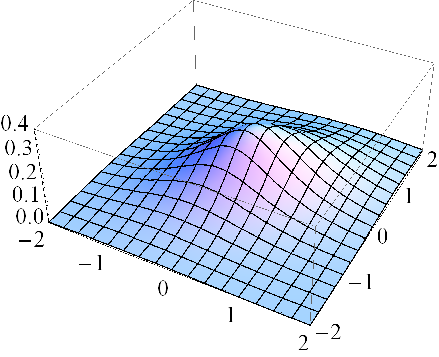
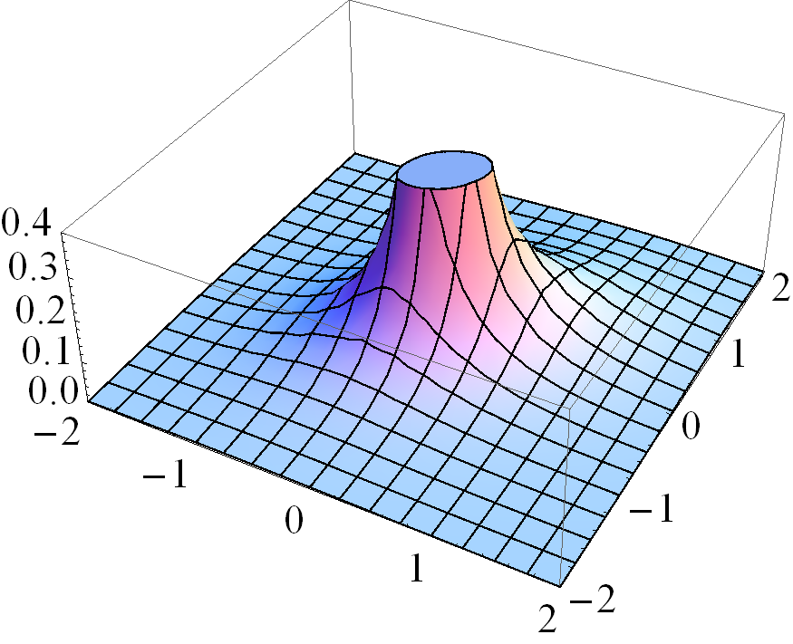
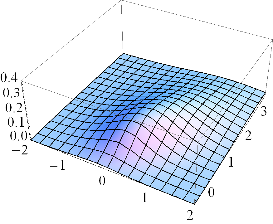
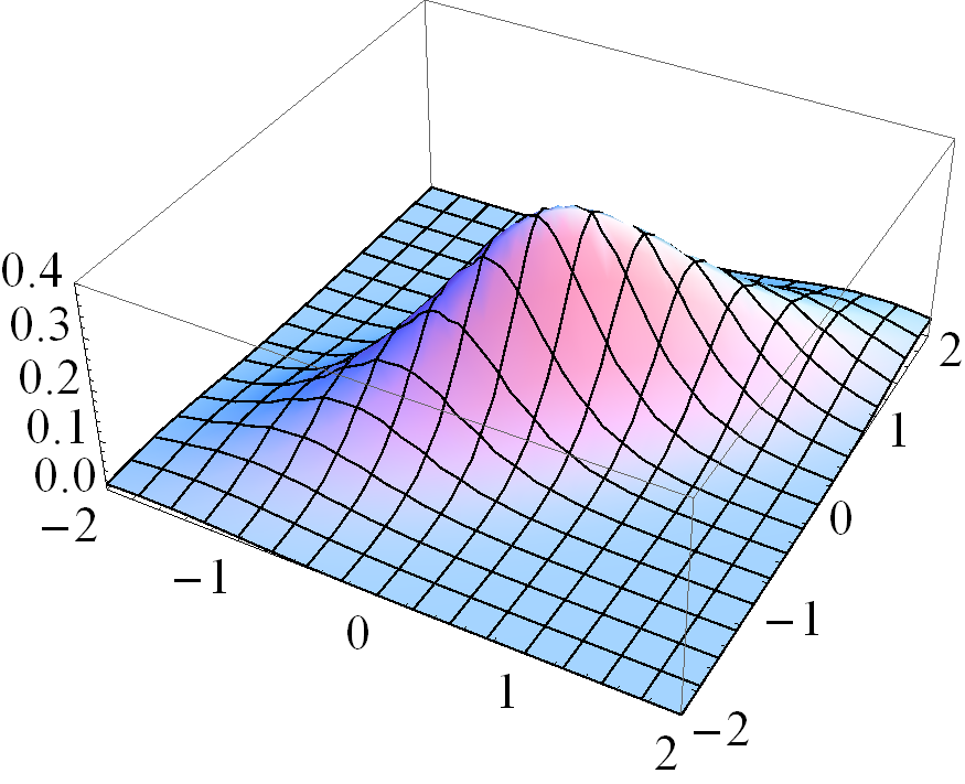
Figure 1 gives four pairs of contour and three dimensional plots for various cases of the MSVG distribution. The first pair of plots is based on parameters

\bm{\mu}=\begin{pmatrix}0\\ 0\end{pmatrix},\quad\bm{\Sigma}=\begin{pmatrix}1&0.4\\ 0.4&1\end{pmatrix},\quad\bm{\gamma}=\begin{pmatrix}0.2\\ 0.3\end{pmatrix},\ \text{and}\ \quad\nu=3.

Based on the distribution for the first pair of plots, three other pairs of plots demonstrate the changes in pdf when the shape parameter decreases to $\nu=0.6$ , the skewness parameter increases to $\bm{\gamma}=(0.5,2)$ , and the correlation coefficient in $\bm{\Sigma}$ increases to 0.8, respectively, while keeping other parameters fixed. Note that the density for the case with small $\nu$ is unbounded.

Refer to caption — (a) standard contour plot

3 ECM Algorithm

In the likelihood approach, maximising the complicated density in (1) can be computationally intensive. We propose the ECM algorithm in the likelihood approach because the normal mean-variance mixtures representation in (2) can greatly simplify the maximisation procedures in the M-step of the algorithm. Then we extend the algorithm to incorporate an AR(1) term and discuss some technical issues involving small $\nu$ .

3.1 Basic algorithm

The ML estimates for parameters $\bm{\theta}=(\bm{\mu},\bm{\Sigma},\bm{\gamma},\nu)$ in the parameter space $\bm{\Theta}$ maximises the log-likelihood

\ell(\bm{\theta}|\bm{y}_{1},...,\bm{y}_{n})=\sum_{i=1}^{n}\log f_{VG}(\bm{y}_{i}|\bm{\theta})

where $f_{VG}(\cdot)$ is the pdf of MSVG distribution in (1). Using the normal mean-variance mixtures representation of the MSVG distribution in (2), we consider $\bm{\lambda}=\{\lambda_{1},...,\lambda_{n}\}$ to be unobserved and $\{\bm{y},\bm{\lambda}\}$ to be the complete data where $\bm{y}=(\bm{y}_{1},...,\bm{y}_{n})$ . The complete data density can be represented as a product of conditional normal densities given the unobserved mixing parameters and the gamma densities of the mixing parameters, that is,

f(\bm{y},\bm{\lambda}|\bm{\theta})=\prod_{i=1}^{n}f_{N}(\bm{y}_{i}|\lambda_{i},\bm{\mu},\bm{\Sigma},\bm{\gamma})f_{G}(\lambda_{i}|\nu).

This is essentially a state space model with normals as the structural distributions, $\lambda_{i}$ as the state or missing parameters, and gamma as the mixing distribution. Due to the mixing structure, the complete-data log-likelihood function can be factorised into two distinct functions as follows:

\displaystyle\ell(\bm{\theta}|\bm{y},\bm{\lambda})=\ell_{N}(\bm{\mu},\bm{\Sigma},\bm{\gamma}|\bm{y},\bm{\lambda})+\ell_{G}(\nu|\bm{\lambda})

(4)

where the log-likelihood of the conditional normal distributions is given by:

\displaystyle\ell_{N}(\bm{\mu},\bm{\Sigma},\bm{\gamma}|\bm{y},\bm{\lambda})=-\frac{n}{2}\log|\bm{\Sigma}|-\frac{1}{2}\sum_{i=1}^{n}\frac{1}{\lambda_{i}}(\bm{y}_{i}-\bm{\mu}-\lambda_{i}\bm{\gamma})^{\prime}\bm{\Sigma}^{-1}(\bm{y}_{i}-\bm{\mu}-\lambda_{i}\bm{\gamma})+C_{1}

(5)

for some constant $C_{1}$ and the log-likelihood of the conditional gamma distributions is given by:

\displaystyle\ell_{G}(\nu|\bm{\lambda})=n\nu\log\nu-n\log\Gamma(\nu)+(\nu-1)\sum_{i=1}^{n}\log\lambda_{i}-\nu\sum_{i=1}^{n}\lambda_{i}.

(6)

Hence, condition on $\bm{\lambda}$ , the estimation of all parameters $(\bm{\mu},\bm{\Sigma},\bm{\gamma},\nu)$ can be separated in two blocks: the conditional maximisation (CM) of $(\bm{\mu},\bm{\Sigma},\bm{\gamma})$ from the conditional normals log-likelihood function and the CM of $\nu$ from the gamma log-likelihood function. The mixing parameter $\bm{\lambda}$ is first estimated by the conditional expectation given the observed-data $\bm{y}$ . The procedures are described as below:

E-step for $\lambda_{i}$ :
To derive the conditional expectations of the $\lambda_{i}$ ’s given the observed-data $\bm{y}_{i}$ and parameters $(\bm{\mu},\bm{\Sigma},\bm{\gamma},\nu)$ , we need the conditional posterior distribution of $\lambda_{i}$ given by:

	$\displaystyle f(\lambda_{i}\|\bm{y}_{i},\bm{\mu},\bm{\Sigma},\bm{\gamma},\nu)\propto$	$\displaystyle\ f(\lambda_{i},\bm{y}_{i}\|\bm{\mu},\bm{\Sigma},\bm{\gamma},\nu)$
	$\displaystyle\propto$	$\displaystyle\ \lambda_{i}^{\nu-\frac{d}{2}-1}\exp\left[-\frac{1}{2\lambda_{i}}(\bm{y}_{i}-\bm{\mu})^{\prime}\bm{\Sigma}^{-1}(\bm{y}_{i}-\bm{\mu})-\frac{\lambda_{i}}{2}\left(\bm{\gamma}^{\prime}\bm{\Sigma}^{-1}\bm{\gamma}+2\nu\right)\right]$		(7)

which corresponds to the pdf of a generalised inverse Gaussian distribution (Embrechts,, 1983). Using this posterior distribution, we can calculate the following conditional expectations:

$\displaystyle\widehat{\lambda_{i}}=$	$\displaystyle\ \mathbb{E}\left(\lambda_{i}\|\bm{y},\bm{\theta}\right)=\frac{\delta_{i}K_{\nu-\frac{d}{2}+1}\left(\sqrt{2\nu+\bm{\gamma}^{\prime}\bm{\Sigma}^{-1}\bm{\gamma}}\delta_{i}\right)}{\sqrt{2\nu+\bm{\gamma}^{\prime}\bm{\Sigma}^{-1}\bm{\gamma}}K_{\nu-\frac{d}{2}}\left(\sqrt{2\nu+\bm{\gamma}^{\prime}\bm{\Sigma}^{-1}\bm{\gamma}}\delta_{i}\right)},$	(8)
$\displaystyle\widehat{1/\lambda_{i}}=$	$\displaystyle\ \mathbb{E}\left(\frac{1}{\lambda_{i}}\Bigg{\|}\bm{y},\bm{\theta}\right)=\frac{\sqrt{2\nu+\bm{\gamma}^{\prime}\bm{\Sigma}^{-1}\bm{\gamma}}K_{\nu-\frac{d}{2}-1}\left(\sqrt{2\nu+\bm{\gamma}^{\prime}\bm{\Sigma}^{-1}\bm{\gamma}}\delta_{i}\right)}{\delta_{i}K_{\nu-\frac{d}{2}}\left(\sqrt{2\nu+\bm{\gamma}^{\prime}\bm{\Sigma}^{-1}\bm{\gamma}}\delta_{i}\right)},$	(9)
$\displaystyle\widehat{\log\lambda_{i}}=$	$\displaystyle\ \mathbb{E}\left(\log\lambda_{i}\|\bm{y},\bm{\theta}\right)=\log\left(\frac{\delta_{i}}{\sqrt{2\nu+\bm{\gamma}^{\prime}\bm{\Sigma}^{-1}\bm{\gamma}}}\right)+\frac{K_{\nu-\frac{d}{2}}^{(1,0)}(\sqrt{2\nu+\bm{\gamma}^{\prime}\bm{\Sigma}^{-1}\bm{\gamma}}\delta_{i})}{K_{\nu-\frac{d}{2}}(\sqrt{2\nu+\bm{\gamma}^{\prime}\bm{\Sigma}^{-1}\bm{\gamma}}\delta_{i})}$	(10)

where $\displaystyle K_{\nu}^{(1,0)}(z)=\tfrac{\partial}{\partial\alpha}K_{\alpha}(z)\big{|}_{\alpha=\nu}$ which is approximated using the central difference formula

K_{\nu}^{(1,0)}(z)\approx\frac{K_{\nu+h}(z)-K_{\nu-h}(z)}{2h}

(11)

where we let $h=10^{-5}$ .

CM-step for $(\bm{\mu},\bm{\Sigma},\bm{\gamma})$ :
Given the mixing parameters $\bm{\lambda}$ , the ML estimate of $(\bm{\mu},\bm{\Sigma},\bm{\gamma})$ can be obtained by maximising $\ell_{N}(\bm{\mu},\bm{\Sigma},\bm{\gamma}|\bm{y},\bm{\lambda})$ in (5) with respect to $(\bm{\mu},\bm{\Sigma},\bm{\gamma})$ . After equating each component of the partial derivatives of $\ell_{N}(\bm{\mu},\bm{\Sigma},\bm{\gamma}|\nu,\bm{y},\bm{\lambda})$ to zero, we obtain the following estimates:

$\displaystyle\hat{\bm{\mu}}=$	$\displaystyle\frac{S_{\bm{y}/\lambda}S_{\lambda}-nS_{\bm{y}}}{S_{1/\lambda}S_{\lambda}-n^{2}},$	(12)
$\displaystyle\hat{\bm{\gamma}}=$	$\displaystyle\frac{S_{\bm{y}}-n\hat{\bm{\mu}}}{S_{\lambda}},$	(13)
$\displaystyle\hat{\bm{\Sigma}}=$	$\displaystyle\frac{1}{n}\sum_{i=1}^{n}\frac{1}{\lambda_{i}}(\bm{y}_{i}-\hat{\bm{\mu}})(\bm{y}_{i}-\hat{\bm{\mu}})^{\prime}-\frac{1}{n}\hat{\bm{\gamma}}\hat{\bm{\gamma}}^{\prime}S_{\lambda},$	(14)

where the complete data sufficient statistics are

\displaystyle S_{\bm{y}}=\sum_{i=1}^{n}\bm{y}_{i},\quad S_{\bm{y}/\lambda}=\sum_{i=1}^{n}\frac{1}{\lambda_{i}}\bm{y}_{i},\quad S_{\lambda}=\sum_{i=1}^{n}\lambda_{i},\quad S_{1/\lambda}=\sum_{i=1}^{n}\frac{1}{\lambda_{i}}.

(15)

CM-step for $\nu$ :
Given the mixing parameters $\bm{\lambda}$ , the ML estimate of $\nu$ can be obtained by numerically maximising $\ell_{G}(\nu|\bm{\lambda})$ in (6) with respect to $\nu$ using Newton-Raphson (NR) algorithm where the derivatives is given by:

	$\displaystyle\frac{\partial\ell}{\partial\nu}=$	$\displaystyle\ n+n\log\nu-n\psi(\nu)+S_{\log\lambda}-S_{\lambda},$		(16)
	$\displaystyle\frac{\partial^{2}\ell}{\partial\nu^{2}}=$	$\displaystyle\ \frac{n}{\nu}-n\psi^{\prime}(\nu).$		(17)

where $\psi(x)=\frac{d}{dx}\log\Gamma(x)$ is the digamma function and $S_{\log\lambda}=\sum_{i=1}^{n}\log\lambda_{i}$ . This ECM algorithm is the MCECM algorithm. In summary, the algorithm involves the following steps:

Initialisation step: Choose suitable starting values $(\bm{\mu}_{0},\bm{\Sigma}_{0},\bm{\gamma}_{0},\nu_{0})$ for the parameters. If the data is roughly symmetric around the mean, then it is recommended to choose starting values $(\bar{\bm{y}},\bm{Q}_{y},\bm{0},d)$ where $\bar{\bm{y}}$ and $\bm{Q}_{y}$ denote the sample mean and sample variance-covariance matrix of $\bm{y}$ respectively.

At the $t$ -th iteration with current estimates $(\bm{\mu}^{(t)},\bm{\Sigma}^{(t)},\bm{\gamma}^{(t)},\nu^{(t)})$ ,

E-step 1: Calculate $\widehat{\lambda}_{i}^{(t+1/2)}$ and $\widehat{1/\lambda_{i}}^{(t+1/2)}$ for $i=1,...,n$ in (8) and (9), respectively, using $(\bm{\mu}^{(t)},\bm{\Sigma}^{(t)},\bm{\gamma}^{(t)},\nu^{(t)})$ . Calculate also the sufficient statistics $S_{\bm{y}/\lambda}^{(t+1/2)}$ , $S_{\lambda}^{(t+1/2)}$ and $S_{1/\lambda}^{(t+1/2)}$ in (15).

CM-step 1: Update the estimates to $(\bm{\mu}^{(t+1)},\bm{\Sigma}^{(t+1)},\bm{\gamma}^{(t+1)})$ in (12) to (14) respectively using the sufficient statistics.

E-step 2: Calculate $\widehat{\lambda_{i}}^{(t+1)}$ and $\widehat{\log\lambda_{i}}^{(t+1)}$ for $i=1,...,n$ in (8) and (10) respectively using the updated estimates $(\bm{\mu}^{(t+1)},\bm{\Sigma}^{(t+1)},\bm{\gamma}^{(t+1)},\nu^{(t)})$ . Calculate also the sufficient statistics $S_{\lambda}^{(t+1)}$ and $S_{\log\lambda}^{(t+1)}$ in (15).

CM-step 2: Update the estimate to $\nu^{(t+1)}$ using the derivatives in (16) and (17) for the NR procedure and the sufficient statistics.

Stopping rule: Repeat the procedures until the relative increment of log-likelihood function is smaller than the tolerance level $10^{-8}$ .

Alternatively, the ECME algorithm update the estimate to $\nu^{(t+1)}$ in CM-step 2 by maximising directly the actual log-likelihood $\ell_{VG}(\nu|\bm{y},\bm{\mu},\bm{\Sigma},\bm{\gamma})$ which is the sum of log pdfs in (1) for $(\bm{y}_{1},\dots,\bm{y}_{n})$ . This procedure is implemented using the optimize function specified in R which is a combination of golden section search and successive parabolic interpolation.

3.2 Algorithm with AR term

Suppose now our observed-data is $\bm{y}=(\bm{y}_{0},...,\bm{y}_{n})$ . The MSVG distribution for $\bm{y}_{i}$ where $i=1,...,n$ with AR mean function of order 1 (without loss of generosity) can be represented hierarchically as follows:

\bm{y}_{i}|\lambda_{i}\sim\mathcal{N}_{d}(\bm{\beta}_{0}+\bm{\beta}_{1}\bm{y}_{i-1}+\bm{\gamma}\lambda_{i},\lambda_{i}\bm{\Sigma}),\quad\lambda_{i}\sim\mathcal{G}(\nu,\nu)

(18)

where $\bm{\beta}_{0}\in\mathbb{R}^{d}$ , and $\bm{\beta}_{1}$ is a $d\times d$ matrix with all eigenvalues less than 1 in modulus. Because of the dependency structure, we maximise the conditional likelihood function for $\bm{y}_{1},...,\bm{y}_{n}$ given $\bm{y}_{0}$ expressed by:

\displaystyle f(\bm{y}_{1},...,\bm{y}_{n},\lambda_{1},...,\lambda_{n}|\bm{y}_{0};\bm{\theta})=

\displaystyle\prod_{i=1}^{n}f_{N}(\bm{y}_{i}|\lambda_{i},\bm{y}_{i-1};\bm{\theta})f_{G}(\lambda_{i};\nu).

So the conditional log-likelihood is given by:

\ell_{c}(\bm{\theta}|\bm{y},\bm{\lambda})=\ell_{N}(\bm{\beta}_{0},\bm{\beta}_{1},\bm{\Sigma},\bm{\gamma}|\bm{y},\bm{\lambda})+\ell_{G}(\nu|\bm{\lambda})

where the log-likelihood of the conditional normal distribution is given by:

	$\displaystyle\ell_{N}(\bm{\beta}_{0},\bm{\beta}_{1},\bm{\Sigma},\bm{\gamma}\|\bm{y},\bm{\lambda})$
	$\displaystyle\hskip 28.45274pt=-\frac{n}{2}\log\|\bm{\Sigma}\|-\frac{1}{2}\sum_{i=1}^{n}\frac{1}{\lambda_{i}}(\bm{y}_{i}-\bm{\beta}_{0}-\bm{\beta}_{1}\bm{y}_{i-1}-\lambda_{i}\bm{\gamma})^{\prime}\bm{\Sigma}^{-1}(\bm{y}_{i}-\bm{\beta}_{0}-\bm{\beta}_{1}\bm{y}_{i-1}-\lambda_{i}\bm{\gamma})+C_{2}$		(19)

for some constant $C_{2}$ and $\ell_{G}(\nu|\bm{\lambda})$ is given in equation (6).

E-step for $\lambda_{i}$ :
This step is similar to the E-step in Section 3.1. Just replace $\delta_{i}^{2}=\left(\bm{y}_{i}-\bm{\mu}\right)^{\prime}\bm{\Sigma}^{-1}\left(\bm{y}_{i}-\bm{\mu}\right)$ with $\delta_{i}^{2}=\left(\bm{y}_{i}-\bm{\beta}_{0}-\bm{\beta}_{1}\bm{y}_{i-1}\right)^{\prime}\bm{\Sigma}^{-1}\left(\bm{y}_{i}-\bm{\beta}_{0}-\bm{\beta}_{1}\bm{y}_{i-1}\right)$ .

CM-step for $(\bm{\beta}_{0},\bm{\beta}_{1},\bm{\Sigma},\bm{\gamma})$ :
Similarly condition on $\lambda_{i}$ , the ML estimates of $(\bm{\beta}_{0},\bm{\beta}_{1},\bm{\Sigma},\bm{\gamma})$ can be obtained by maximising $\ell_{N}(\bm{\beta}_{0},\bm{\beta}_{1},\bm{\Sigma},\bm{\gamma}|\bm{y},\bm{\lambda})$ in (19) with respect to $(\bm{\beta}_{0},\bm{\beta}_{1},\bm{\Sigma},\bm{\gamma})$ . This gives us a close form solution as follows:

	$\displaystyle\begin{pmatrix}\hat{\bm{\beta}_{0}^{\prime}}\\ \hat{\bm{\beta}_{1}^{\prime}}\\ \hat{\bm{\gamma}^{\prime}}\end{pmatrix}=$	$\displaystyle\begin{pmatrix}S_{1/\lambda}&S^{\prime}_{\bm{x}/\lambda}&n\\ S_{\bm{x}/\lambda}&S_{\bm{x}\bm{x}^{\prime}/\lambda}&S_{\bm{x}}\\ n&S^{\prime}_{\bm{x}}&S_{\lambda}\end{pmatrix}^{-1}\begin{pmatrix}S^{\prime}_{\bm{y}/\lambda}\\ S_{\bm{x}\bm{y}^{\prime}/\lambda}\\ S^{\prime}_{\bm{y}}\end{pmatrix}$		(20)
	$\displaystyle\hat{\bm{\Sigma}}=$	$\displaystyle\ \frac{1}{n}\sum_{i=1}^{n}\frac{1}{\lambda_{i}}(\bm{y}_{i}-\bm{\beta}_{0}-\bm{\beta}_{1}\bm{y}_{i-1})(\bm{y}_{i}-\bm{\beta}_{0}-\bm{\beta}_{1}\bm{y}_{i-1})^{\prime}-\frac{1}{n}\bm{\gamma}\bm{\gamma}^{\prime}S_{\lambda},$		(21)

where (20) as a generalisation of (12) and (13) can be further generalised to include higher order AR terms in the mean function. Then the complete data sufficient statistics are given by (15) with the addition of

\displaystyle S_{\bm{x}}=\sum_{i=1}^{n}\bm{y}_{i-1},\ S_{\bm{x}/\lambda}=\sum_{i=1}^{n}\frac{1}{\lambda_{i}}\bm{y}_{i-1},\ S_{\bm{x}\bm{x}^{\prime}/\lambda}=\sum_{i=1}^{n}\frac{1}{\lambda_{i}}\bm{y}_{i-1}\bm{y}_{i-1}^{\prime},\ S_{\bm{x}\bm{y}^{\prime}/\lambda}=\sum_{i=1}^{n}\frac{1}{\lambda_{i}}\bm{y}_{i-1}\bm{y}_{i}^{\prime}.

(22)

CM-step for $\nu$ :
This step is the same as in Section 3.1.

In summary, the layout of the MCECM and ECME algorithms are similar to those for the MSVG model in Section 3.1 except that we update $\bm{\beta}_{0}$ and $\bm{\beta}_{1}$ instead of $\bm{\mu}$ and adjust the E-step accordingly.

3.3 Adjustment to ECM algorithm

3.3.1 Adjustment for small $\nu$

Numerical problems may occur when dealing with $\nu\leq\tfrac{d}{2}$ since the pdf $f_{VG}(\bm{y}_{i})$ in (1) at $\bm{\mu}$ is unbounded for such $\nu$ . To handle such case, we can show that as $\bm{y}_{i}\rightarrow\bm{\mu}$ ,

$\displaystyle\mathbb{E}(\lambda_{i}\|\bm{y}_{i},\bm{\theta})$	$\displaystyle\sim$	$\displaystyle\begin{cases}\frac{2\nu-d}{2\nu+\bm{\gamma}^{\prime}\bm{\Sigma}^{-1}\bm{\gamma}}&\text{ if }\nu>\tfrac{d}{2},\\ -\frac{1}{(2\nu+\bm{\gamma}^{\prime}\bm{\Sigma}^{-1}\bm{\gamma})\log\delta_{i}}&\text{ if }\nu=\tfrac{d}{2},\\ \frac{\Gamma(\nu-\tfrac{d}{2}+1)}{\Gamma(\tfrac{d}{2}-\nu)}2^{2\nu-d+1}\left(2\nu+\bm{\gamma}^{\prime}\bm{\Sigma}^{-1}\bm{\gamma}\right)^{\frac{d}{2}-\nu-1}\delta_{i}^{d-2\nu}&\text{ if }\nu<\tfrac{d}{2},\\ \end{cases}$
$\displaystyle\mathbb{E}\left(\frac{1}{\lambda_{i}}\Bigg{\|}\bm{y}_{i},\bm{\theta}\right)$	$\displaystyle\sim$	$\displaystyle\begin{cases}\frac{2\nu+\bm{\gamma}^{\prime}\bm{\Sigma}^{-1}\bm{\gamma}}{2\nu-d-2}&\text{ if }\nu>\tfrac{d}{2}+1,\\ -\left(2\nu+\bm{\gamma}^{\prime}\bm{\Sigma}^{-1}\bm{\gamma}\right)\log\delta_{i}&\text{ if }\nu=\tfrac{d}{2}+1,\\ \frac{\Gamma(1-\nu+\tfrac{d}{2})}{\Gamma(\nu-\tfrac{d}{2})}2^{1-2\nu+d}\left(2\nu+\bm{\gamma}^{\prime}\bm{\Sigma}^{-1}\bm{\gamma}\right)^{\nu-\frac{d}{2}}\delta_{i}^{2\nu-d-2}&\text{ if }\nu\in(\tfrac{d}{2},\tfrac{d}{2}+1),\\ -\frac{1}{\delta_{i}^{2}\log\delta_{i}}&\text{ if }\nu=\tfrac{d}{2},\\ \frac{d-2\nu}{\delta_{i}^{2}}&\text{ if }\nu<\tfrac{d}{2},\\ \end{cases}$
$\displaystyle\mathbb{E}(\log\lambda_{i}\|\bm{y}_{i},\bm{\theta})$	$\displaystyle\sim$	$\displaystyle\begin{cases}\psi(\nu-\frac{d}{2})-\log\left(\frac{2\nu+\bm{\gamma}^{\prime}\bm{\Sigma}^{-1}\bm{\gamma}}{2}\right)&\text{ if }\nu>\tfrac{d}{2},\\ \log\delta_{i}&\text{ if }\nu=\tfrac{d}{2},\\ 2\log\delta_{i}&\text{ if }\nu<\tfrac{d}{2}.\end{cases}$

So for $\nu\leq\tfrac{d}{2}+1$ and $\nu\leq\tfrac{d}{2}$ , $\mathbb{E}(\frac{1}{\lambda_{i}}|\delta_{i},\bm{\gamma},\nu)$ and $\mathbb{E}(\log\lambda_{i}|\delta_{i},\bm{\gamma},\nu)$ are unbounded for data points at the mean $\bm{\mu}$ respectively. As these expected values are numerically unstable to calculate, we propose to bound the pdf around $\bm{\mu}$ by a bound such that if

\displaystyle\delta_{i}\sqrt{2\nu+\bm{\gamma}^{\prime}\bm{\Sigma}^{-1}\bm{\gamma}}<\Delta,

(23)

where $\Delta$ is a small fixed constant, then we compute the expected values $\mathbb{E}(\frac{1}{\lambda_{i}}|\delta_{i}^{*},\bm{\gamma},\nu)$ and $\mathbb{E}(\log\lambda_{i}|\delta_{i}^{*},\bm{\gamma},\nu)$ in (9) and (10) with $\delta_{i}^{*}=\Delta/\sqrt{2\nu+\bm{\gamma}^{\prime}\bm{\Sigma}^{-1}\bm{\gamma}}$ replacing $\delta_{i}$ . The region in (23) will be called the delta region. We will analyse the optimal choices of $\Delta$ in a simulation study in the next section.

Another problem may occur when estimating $\bm{\Sigma}$ . Suppose that $\bm{y}_{i}\rightarrow\bm{\mu}^{(t)}$ for some $i$ , then $\widehat{1/\lambda_{i}}^{(t+1/2)}\rightarrow\infty$ . Now consider the CM-step for $(\bm{\mu},\bm{\Sigma},\bm{\gamma})$ , $\bm{\mu}^{(t+1)}$ needs to be calculated before calculating $\bm{\Sigma}^{(t+1)}$ . For the $i\textsuperscript{th}$ term of the first summation for calculating $\bm{\Sigma}^{(t+1)}$ in (14), we get that

\displaystyle\widehat{1/\lambda_{i}}^{(t+1/2)}(\bm{y}_{i}-\bm{\mu}^{(t+1)})(\bm{y}_{i}-\bm{\mu}^{(t+1)})^{\prime}\rightarrow\infty,

which leads to $\bm{\Sigma}^{(t+1)}$ diverging to infinity since $(\bm{y}_{i}-\bm{\mu}^{(t+1)})$ does not converge to zero. To solve this problem, we insert an extra E-step to update $\widehat{1/\lambda_{i}}^{(t+3/4)}$ and $\widehat{\lambda}_{i}^{(t+3/4)}$ after updating $(\bm{\mu}^{(t+1)},\bm{\gamma}^{(t+1)})$ . This adjustment makes the $i\textsuperscript{th}$ term of the first summation in $\bm{\Sigma}^{(t+1)}$ to be

\displaystyle\widehat{1/\lambda_{i}}^{(t+3/4)}(\bm{y}_{i}-\hat{\bm{\mu}}^{(t+1)})(\bm{y}_{i}-\hat{\bm{\mu}}^{(t+1)})^{\prime}\rightarrow\bm{C}

for some finite constant matrix $\bm{C}$ resulting in a more numerically stable estimate for $\bm{\Sigma}^{(t+1)}$ . Thus adding an additional E-step to update $\widehat{1/\lambda_{j}}^{(t+3/4)}$ after updating $\bm{\mu}^{(t+1)}$ and $\bm{\gamma}^{(t+1)}$ before updating $\bm{\Sigma}^{(t+1)}$ improves the numerical stability and convergence of the algorithm.

3.3.2 Hybrid ECM algorithm

Meng and Rubin, (1993), Liu and Rubin, (1994) together showed that the MCECM and ECME algorithm always increase the log-likelihood monotonically. However, problems might occur when dealing with multimodel log-likelihood such as the MSVG log-likelihood when $\nu\leq\frac{d}{2}$ .

In the MCECM algorithm, $\nu$ is estimated by numerically maximising the log-likelihood of the conditional gamma mixing density using NR algorithm with derivatives (16) and (17). The ECME algorithm which numerically maximises the actual log-likelihood of the MSVG distribution with pdf (1), is computationally less efficient than the MCECM algorithm despite less iterations are required for convergence. However, the ECME algorithm is more stable than the MCECM algorithm since the CM-step for $\nu$ maximises the actual log-likelihood, hence avoiding the missing data $\widehat{\log\lambda}_{i}$ in CM-step 2.

In light of this, we propose an algorithm which combines the efficiency of the MCECM algorithm while maintaining the performance of the ECME algorithm. We call this the hybrid ECM (HECM) algorithm. Essentially it starts with the MCECM algorithm and repeats until either the relative increment of log-likelihood is smaller than $10^{-8}$ which stops the algorithm, reverts back to the previous estimates and performs the ECME algorithm.

For the univariate skew VG model, the performance of the HECM algorithm can be improved by replacing the estimate for $\hat{\mu}$ in (12) with the estimate for $\mu$ such that it maximizes the actual log-likelihood $\ell_{VG}(\mu|\bm{y},\sigma^{2},\gamma,\nu)$ .

The two adjustments using density bound and extra E-step as well as the hybrid procedures balance computational efficiency, and accuracy of the ML estimation.

3.4 Observed Information Matrix

Letting $\bm{Y}_{c}=(\bm{y},\bm{\lambda})$ be the complete data, Louis, (1982) expressed the observed information matrix $\bm{I}_{o}(\bm{\theta})$ in terms of the conditional expectation of the derivatives of complete data log-likelihood $\ell^{\prime}(\bm{\theta}|\bm{Y}_{c})$ and $\ell^{\prime\prime}(\bm{\theta}|\bm{Y}_{c})$ with respect to conditional distribution $\bm{\lambda}|\bm{y}$ which depends on $\bm{\theta}$ :

\bm{I}_{o}(\bm{\theta})=-\mathbb{E}_{\bm{\theta}}[\ell^{\prime\prime}(\bm{\theta}|\bm{Y}_{c})]-\mathbb{E}_{\bm{\theta}}[\ell^{\prime}(\bm{\theta}|\bm{Y}_{c})\ell^{\prime T}(\bm{\theta}|\bm{Y}_{c})]+\mathbb{E}_{\bm{\theta}}[\ell^{\prime}(\bm{\theta}|\bm{Y}_{c})]\mathbb{E}_{\bm{\theta}}[\ell^{\prime}(\bm{\theta}|\bm{Y}_{c})]^{T}.

(24)

In the context of MSVG model, $\ell(\bm{\theta}|\bm{Y}_{c})$ is given by (4). The first derivatives of complete data log-likelihood can be expressed as

	$\displaystyle\frac{\partial\ell_{N}}{\partial\bm{\beta}_{0}}=\bm{\Sigma}^{-1}\sum_{i=1}^{n}\frac{1}{\lambda_{i}}(\bm{y}_{i}-\bm{\beta}_{0}-\bm{\beta}_{1}\bm{y}_{i-1}-\lambda_{i}\bm{\gamma})$
	$\displaystyle\frac{\partial\ell_{N}}{\partial\text{vec}\bm{\beta}_{1}}=\text{vec}\left[\bm{\Sigma}^{-1}\sum_{i=1}^{n}\frac{1}{\lambda_{i}}(\bm{y}_{i}-\bm{\beta}_{0}-\bm{\beta}_{1}\bm{y}_{i-1}-\lambda_{i}\bm{\gamma})\bm{y}_{i-1}^{\prime}\right]$
	$\displaystyle\frac{\partial\ell_{N}}{\partial\text{vech}\bm{\Sigma}}=\text{vech}\left(2(\bm{1}_{p\times p})-\bm{I}\right)\circ\text{vech}\left(-\frac{n}{2}\bm{\Sigma}^{-1}+\frac{1}{2}\bm{\Sigma}^{-1}S_{\tilde{\bm{y}}\tilde{\bm{y}}^{\prime}/\lambda}\bm{\Sigma}^{-1}\right)$
	$\displaystyle\frac{\partial\ell_{N}}{\partial\bm{\gamma}}=\bm{\Sigma}^{-1}\sum_{i=1}^{n}(\bm{y}_{i}-\bm{\beta}_{0}-\bm{\beta}_{1}\bm{y}_{i-1}-\lambda_{i}\bm{\gamma})$
	$\displaystyle\frac{\partial\ell_{G}}{\partial\nu}=n+n\log\nu-n\psi(\nu)+\sum_{i=1}^{n}\log\lambda_{i}-\sum_{i=1}^{n}\lambda_{i}$

where $\text{vec}(\cdot)$ and $\text{vech}(\cdot)$ are the vectorisation and half-vectorisation operators respectively, $\bm{1}_{p\times p}$ is the $p\times p$ matrix of 1’s, $\bm{I}$ be a conformable identity matrix, and

\displaystyle S_{\tilde{\bm{y}}\tilde{\bm{y}}^{\prime}/\lambda}=

\displaystyle\sum_{i=1}^{n}\frac{1}{\lambda_{i}}(\bm{y}_{i}-\bm{\beta}_{0}-\bm{\beta}_{1}\bm{y}_{i-1}-\lambda_{i}\bm{\gamma})(\bm{y}_{i}-\bm{\beta}_{0}-\bm{\beta}_{1}\bm{y}_{i-1}-\lambda_{i}\bm{\gamma})^{\prime}.

Calculating the conditional expectations in equation (24) requires the second order derivatives which can be obtained using vector differentiation, and the following conditional expectations

	$\displaystyle\mathbb{E}_{\bm{\theta}}\left(\lambda_{i}^{k}\right)=$	$\displaystyle\left(\frac{\delta_{i}}{\psi}\right)^{k}\frac{K_{\nu-\frac{d}{2}+k}\left(\delta_{i}\psi\right)}{K_{\nu-\frac{d}{2}}\left(\delta_{i}\psi\right)}$
	$\displaystyle\mathbb{E}_{\bm{\theta}}\left(\lambda_{i}^{k}\log\lambda_{i}\right)=$	$\displaystyle\left(\frac{\delta_{i}}{\psi}\right)^{k}\frac{1}{K_{\nu-\frac{d}{2}}\left(\delta_{i}\psi\right)}\left[K^{(1,0)}_{\nu-\frac{d}{2}+k}\left(\delta_{i}\psi\right)+\log\left(\frac{\delta_{i}}{\psi}\right)K_{\nu-\frac{d}{2}+k}\left(\delta_{i}\psi\right)\right]$
	$\displaystyle\mathbb{E}_{\bm{\theta}}\left((\log\lambda_{i})^{2}\right)=$	$\displaystyle\left[\log\left(\frac{\delta_{i}}{\psi}\right)\right]^{2}+\frac{K_{\nu-\frac{d}{2}}^{(2,0)}\left(\delta_{i}\psi\right)+2\log\left(\frac{\delta_{i}}{\psi}\right)K_{\nu-\frac{d}{2}}^{(1,0)}\left(\delta_{i}\psi\right)}{K_{\nu-\frac{d}{2}}\left(\delta_{i}\psi\right)}$

where we let $\psi=\sqrt{\bm{\gamma}^{\prime}\bm{\Sigma}^{-1}\bm{\gamma}+2\nu}$ and $K_{\nu}^{(2,0)}(z)=\tfrac{\partial^{2}}{\partial\alpha^{2}}K_{\alpha}(z)\big{|}_{\alpha=\nu}$ which is approximated using central difference formula.

The asymptotic covariance matrix of $\hat{\bm{\theta}}$ can be approximated by the inverse of the observed information matrix $\bm{I}_{o}(\hat{\bm{\theta}})$ . This gives us a way to approximate the standard error of $\hat{\theta}_{i}=(\hat{\bm{\theta}})_{i}$

SE\left(\hat{\theta_{i}}\right)\approx\sqrt{\left[\bm{I}_{o}(\hat{\bm{\theta}})^{-1}\right]_{ii}}\ .

(25)

4 Simulation Study

We perform three simulation studies: firstly, to compare the efficiency of the MCECM, ECME and HECM algorithms with the extra E-step mentioned in Section 3.3.1; secondly, to analyse the optimal choices of $\Delta$ on increasing the dimension of MSVG distribution; and lastly, to assess the performance of HECM algorithm for different levels of shape and skewness parameters. We use the statistical program called R to generate $r$ random samples from the MSVG distribution each of sample size $n=1000$ and estimate the parameters for each sample. We set the true parameters to be

\bm{\mu}=\begin{pmatrix}0\\ 0\end{pmatrix},\quad\bm{\Sigma}=\begin{pmatrix}1&0.4\\ 0.4&1\end{pmatrix},\quad\bm{\gamma}=\begin{pmatrix}0.2\\ 0.3\end{pmatrix},\quad\nu=3

for the bivariate base model and use initial values recommended in Section 3.1, that is $(\bm{\mu}_{0},\bm{\Sigma}_{0},\bm{\gamma}_{0},\nu_{0})=(\bar{\bm{y}},\bm{Q}_{y},\bm{0},2)$ . To improve convergence, we multiply the data by $C=100$ . Thus we have the scaled parameters as $C\bm{\mu}$ , $C^{2}\bm{\Sigma}$ and $C\bm{\gamma}$ for $\bm{\mu}$ , $\bm{\Sigma}$ and $\bm{\gamma}$ respectively. The results are then rescaled back and for each random sample, we calculate the log-likelihood to assess the model fit.

4.1 Efficiency across algorithms

To illustrate that the three algorithms, MCECM, ECME, and HECM provide good estimates, we perform the simulation above with $r=1000$ replications using the bivariate base model and compare their relative performance. In Table 1 below, the average of parameter estimates, log-likelihoods, number of iterations for convergence over replications, and the total computational times are presented. For each algorithm, we generate the same set of simulated data using the same seed to eliminate the effect of sampling errors in the comparison.

Table 1: Parameter estimates and model efficiency measures across algorithms

	true	MCECM	ECME	HECM
$\mu_{1}$	0	$-$ 0.0072	$-$ 0.0072	$-$ 0.0072
$\mu_{2}$	0	$-$ 0.0069	$-$ 0.0069	$-$ 0.0069
$\Sigma_{1,1}$	1	0.9959	0.9959	0.9959
$\Sigma_{1,2}$	0.4	0.3973	0.3973	0.3973
$\Sigma_{2,2}$	1	0.9914	0.9914	0.9914
$\gamma_{1}$	0.2	0.2067	0.2067	0.2068
$\gamma_{2}$	0.3	0.3062	0.3062	0.3062
$\nu$	2.5	2.5699	2.5709	2.5710
loglik		$-$ 2713.41	$-$ 2713.41	$-$ 2713.41
conv.iter		75.6	31.8	76.6
time (hr)		8.1	16.4	9.1

All estimates obtained are reasonably close to the true value which supports the validity of these algorithms. As expected, MCECM algorithm is the most efficient in terms of computation time whereas ECME algorithm converges the fastest in terms of the number of iterations. However the ECME and HECM algorithms provide slightly better model fits when comparing more digits of the averaged log-likelihood. Overall HECM algorithm is preferred as it provides better model fit than the MCECM algorithm and runs faster than the ECME algorithm. Hence HECM algorithm will be adopted in all subsequent analyses.

4.2 Efficiency across $\Delta$ for small shape parameter

In this simulation study, we analyse the behavior of estimates for different levels of $\Delta$ as defined in Section 3.3.1. We begin the simulation study with bivariate skewed VG distribution with parameters as in Table 1 but with $\nu=0.6$ as the true shape parameter. The shape parameter is chosen to satisfy the condition $\nu\leq\tfrac{d}{2}$ for unbounded density. We repeat the experiment for different levels of $\Delta$ but we do not report average log-likelihood because it can be estimated to be as large as possible by reducing the value of $\Delta$ . For each $\Delta$ level, we repeat the estimation procedure $r=1000$ times. Generally from the results of the experiment as shown in Table 2, the further away the $\Delta$ is from the range (1e-5,1e-3), the further away are the estimates from their true values. Hence, an optimal range of $\Delta$ is from 1e-5 to 1e-3.

This experiment is repeated for dimension $d=3$ with $\nu=1$ . The results for these experiments are given in Tables 3.

Table 2: Parameter estimates across levels of

\Delta

for skewed bivariate VG model.

		$\Delta$ levels
	true	1e-300	1e-100	1e-50	1e-10	1e-7	1e-5	1e-4	1e-3
$\mu_{1}$	0	0.0040	0.0040	0.0040	0.0040	0.0040	0.0040	0.0040	0.0039
$\mu_{2}$	0	0.0058	0.0058	0.0058	0.0058	0.0058	0.0058	0.0058	0.0056
$\Sigma_{1,1}$	1	1.2118	1.0600	1.0434	1.0111	1.0043	0.9997	0.9961	0.9916
$\Sigma_{1,2}$	0.4	0.4880	0.4251	0.4184	0.4054	0.4027	0.4009	0.3994	0.3976
$\Sigma_{2,2}$	1	1.2149	1.0607	1.0438	1.0116	1.0049	1.0003	0.9967	0.9921
$\gamma_{1}$	0.2	0.1939	0.1910	0.1932	0.1952	0.1952	0.1953	0.1951	0.1950
$\gamma_{2}$	0.3	0.2904	0.2861	0.2894	0.2925	0.2925	0.2925	0.2923	0.2921
$\nu$	0.6	0.3300	0.4421	0.4964	0.5771	0.5885	0.5965	0.6010	0.6053
Estimate in bold is closest to the true value.

Table 3: Parameter estimates across levels of

\Delta

for skewed trivariate VG model.

		$\Delta$ levels
	true	1e-7	1e-6	1e-5	1e-4	1e-3	1e-2	1e-1
$\mu_{1}$	0	-0.0019	-0.0019	-0.0019	-0.0019	-0.0019	-0.0018	0.0013
$\mu_{2}$	0	-0.0024	-0.0024	-0.0024	-0.0024	-0.0024	-0.0022	-0.0020
$\mu_{3}$	0	-0.0012	-0.0012	-0.0012	-0.0012	-0.0012	-0.0011	-0.0015
$\Sigma_{1,1}$	1	1.0092	1.0070	1.0049	1.0026	0.9989	0.9952	0.9889
$\Sigma_{1,2}$	0.4	0.4020	0.4012	0.4003	0.3994	0.3980	0.3966	0.3942
$\Sigma_{1,3}$	0.3	0.3019	0.3013	0.3007	0.3000	0.2989	0.2978	0.2960
$\Sigma_{2,2}$	1	1.0094	1.0073	1.0051	1.0029	0.9992	0.9956	0.9893
$\Sigma_{2,3}$	0.2	0.2007	0.2003	0.1999	0.1995	0.1988	0.1981	0.1969
$\Sigma_{3,3}$	1	1.0128	1.0107	1.0086	1.0064	1.0027	0.9991	0.9926
$\gamma_{1}$	0.2	0.2012	0.2012	0.2012	0.2012	0.2010	0.2007	0.1999
$\gamma_{2}$	0.3	0.3026	0.3026	0.3026	0.3026	0.3025	0.3019	0.3013
$\gamma_{3}$	0.4	0.4018	0.4018	0.4018	0.4018	0.4016	0.4010	0.4009
$\nu$	1	0.9512	0.9602	0.9696	0.9795	0.9912	1.0013	1.0225
Estimate in bold is closest to the true value.

On increasing the dimension, the optimal ranges for $\Delta$ is (1e-5,1e-1). As for the subsequent simulation experiment, we implement $\Delta$ within the optimal ranges for dimension 2 to 3. As results show that the optimal $\Delta$ range only increases slowly with $d$ , we apply the optimum $\Delta$ range for $d=3$ to the five dimensional MSVG model in the real data analysis.

For the univariate case, we use the modified HECM algorithm as mentioned in Section 3.3.2. The results are presented below in Table 4. Due to the modification, it is not possible to directly compare the algorithm for high dimensional cases. As the $\Delta$ level gets bigger, $\hat{\sigma}^{2}$ and $\hat{\gamma}$ increases towards the true value. However, $\hat{\nu}$ increases away from the true value. Since the optimal $\Delta$ range is not clear for the univariate case, we suggest any $\Delta$ in the range (1e-10,1e-3).

Table 4: Parameter estimates across levels of

\Delta

for symmetric univariate VG model

		$\Delta$ levels
	true	1e-300	1e-100	1e-50	1e-20	1e-10	1e-5	1e-3
$\mu$	0	0.0000	0.0000	0.0000	0.0000	0.0000	0.0000	0.0000
$\sigma^{2}$	1	0.8564	0.8564	0.8564	0.8564	0.8663	0.8862	0.9148
$\gamma$	0.2	0.1878	0.1878	0.1878	0.1878	0.1885	0.1907	0.1952
$\nu$	0.3	0.3102	0.3102	0.3102	0.3102	0.3111	0.3137	0.3267

4.3 Effects of shape and skewness parameters

In this simulation study, we study the performance of HECM algorithm for various levels of skewness parameter $\bm{\gamma}$ when the shape parameter is $\nu=3$ and $\nu=0.6$ which indicates large and small value respectively according to the condition $\nu\leq\tfrac{d}{2}$ . We consider the same bivariate base model as described at the start of Section 4 except that the true skewness parameters are $\bm{\gamma}$ = (0.2,0.2), (0.5,0.5), (0.7,0.7), (1,1), (2,2) and (0.5,2). We report the averaged iteration in which the algorithm switches from MCECM to ECME algorithm as denoted by switch iter, the averaged iteration when the algorithm converges by conv iter, and the total time it takes to run the algorithm.

Table 5: Parameter estimates and model efficiency measures for

\nu=3

		True $(\gamma_{1},\gamma_{2})$
	true	$(0.2,0.2)$	$(0.5,0.5)$	$(0.7,0.7)$	$(1,1)$	$(2,2)$	$(0.5,2)$
$\mu_{1}$	0	-0.0081	-0.0129	-0.0149	-0.0176	-0.0246	-0.0071
$\mu_{2}$	0	-0.0095	-0.0143	-0.0162	-0.0186	-0.0244	-0.0292
$\Sigma_{1,1}$	1	0.9960	0.9942	0.9927	0.9903	0.9779	0.9951
$\Sigma_{1,2}$	0.4	0.3985	0.3963	0.3947	0.3921	0.3790	0.3932
$\Sigma_{2,2}$	1	0.9952	0.9931	0.9915	0.9888	0.9759	0.9727
$\gamma_{1}$		0.2061	0.5108	0.7128	1.0154	2.0221	0.5050
$\gamma_{2}$		0.2084	0.5131	0.7150	1.0173	2.0229	2.0277
$\nu$	3	3.1006	3.0856	3.0785	3.0699	3.0477	3.0535
switch.iter		99.31	105.34	111.89	125.73	241.16	192.61
conv.iter		99.31	105.34	111.89	125.73	241.16	192.61
time (hr)		11.5	12.1	12.3	22.8	41.2	34.2

Table 5 shows that all estimates are very close to their true values. On increasing the level of skewness, the biases of parameters $\bm{\mu}$ , $\bm{\gamma}$ and $\bm{\Sigma}$ tend to increase gradually while the bias for $\nu$ decreases gradually. The number of iterations to switch and converge and hence the computation time also increase accordingly. This also applies for the unequal skewness case. Moreover, there is no reliance of ECME algorithm as the parameter $\nu$ is chosen so that $\nu>d/2$ . Indeed the simulation with larger skewness needs more iterations for the algorithm to converge. The results when $\nu=0.6$ is presented in Table 6.

Table 6: Parameter estimates and model efficiency measures for

\nu=0.6

		True $(\gamma_{1},\gamma_{2})$
	true	$(0.2,0.2)$	$(0.5,0.5)$	$(0.7,0.7)$	$(1,1)$	$(2,2)$	$(0.5,2)$
$\mu_{1}$	0	0.0043	0.0083	0.0108	0.0136	0.0212	0.0052
$\mu_{2}$	0	0.0042	0.0082	0.0110	0.0138	0.0213	0.0213
$\Sigma_{1,1}$	1	0.9995	1.0054	1.0114	1.0220	1.0573	1.0175
$\Sigma_{1,2}$	0.4	0.4006	0.4061	0.4124	0.4226	0.4391	0.4167
$\Sigma_{2,2}$	1	0.9990	1.0044	1.0111	1.0217	1.0540	1.0558
$\gamma_{1}$		0.1950	0.4904	0.6876	0.9845	2.0337	0.5007
$\gamma_{2}$		0.1943	0.4897	0.6866	0.9835	2.0328	2.0028
$\nu$	0.6	0.5968	0.5961	0.5957	0.5945	0.5946	0.5940
switch.iter		26.8	27.6	28.1	23.7	23.2	26.5
conv.iter		28.4	28.0	28.5	24.5	23.2	26.5
time (hr)		4.9	3.5	3.7	6.7	5.8	6.6

The parameter estimates using HECM algorithm and optimal $\Delta$ to deal with unbounded density are reasonably accurate. This justifies the choice of $\Delta$ for $d=2$ . Surprisingly the algorithm roughly needs around the same number of iterations for each skewness level. In comparison with the results in Table 5 for larger $\nu$ , the algorithm requires significantly less iterations. Eventually, the HECM algorithm switch to ECME to obtain parameter estimates. This justifies our proposed HECM algorithm instead of relying solely on MCECM.

In summary, the proposed HECM algorithm gives good parameter estimates for the MSVG distribution even when its shape parameter is small and skewness is heavy.

5 Real Data Analysis

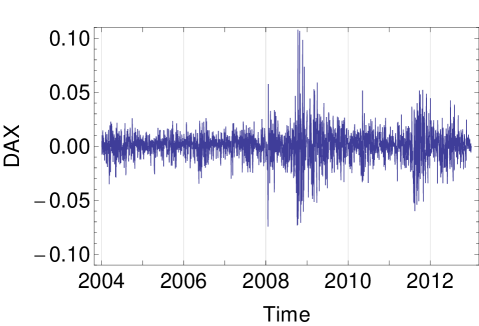
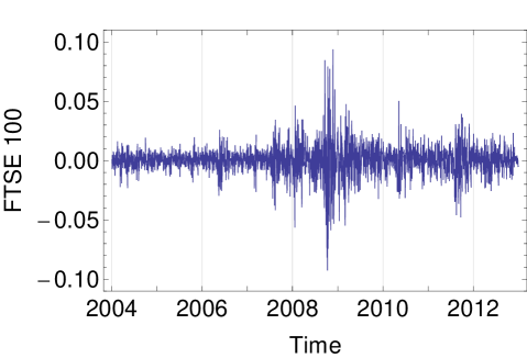
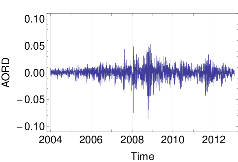
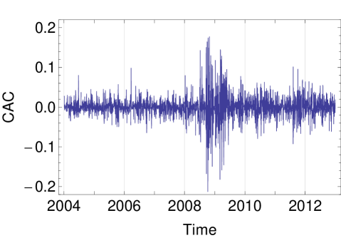
To illustrate the applicability of HECM algorithm using the MSVG AR model, we consider the returns of five daily closing price indices, namely, Deutscher Aktien (DAX), Standard & Poors 500 (S&P 500), Financial Times Stock Exchange 100 (FTSE 100), All Ordinaries (AORD) and Cotation Assiste en Continu 40 (CAC) from 1^st January 2004 to 31^st December 2012 with tolerance level of $10^{-10}$ . After filtering the data with missing closing prices, we obtain the data size of $n=2188$ . Plots of the five time series are given in Figure 2. As the summary statistics in Table 7 show that the data exhibit considerable skewness and kurtosis, we begin our analyses with the MSVG model adopting a constant mean. To assess the model fit, we use the Akaike information criterion with a correction for finite sample size (AICc) given by:

AICc=AIC+\frac{2k(k+1)}{n-k-1}

where $k$ denotes the number of model parameters. Model with the lowest AICc value is preferred as it demonstrates the best model fit after accounting for model complicity.

Table 7: Summary statistics for the five daily return series

${\dagger}$ The reported means are multiplied by 1000.
	DAX	S&P 500	FTSE 100	AORD	CAC
mean^†	0.2901	0.1096	0.1223	0.1587	0.1755
sd	0.0146	0.0136	0.0127	0.0114	0.0287
max	0.1080	0.1096	0.0938	0.0540	0.1778
min	$-$ 0.0774	$-$ 0.0947	$-$ 0.0926	$-$ 0.1049	$-$ 0.2133
skewness	0.0208	$-$ 0.2939	$-$ 0.0946	$-$ 0.7291	0.1524
kurtosis	9.4529	12.9395	11.0138	10.4846	11.7483

The results for the estimated parameters and their standard errors are given in Table 8 .

Table 8: Results for the Multivariate Skewed VG model

	estimate	standard error
$\bm{\mu}^{T}$	$10^{-4}\begin{pmatrix}18&10&12&20&-7\end{pmatrix}$	$10^{-4}\begin{pmatrix}3&3&3&3&6\end{pmatrix}$
$\bm{\Sigma}$	$10^{-5}\begin{pmatrix}19&10&14&5&12\\ &14&8&2&17\\ &&13&4&9\\ &&&12&0.4\\ &&&&66\end{pmatrix}$	$10^{-6}\begin{pmatrix}7&5&6&4&9\\ &5&4&3&9\\ &&5&3&7\\ &&&5&7\\ &&&&26\end{pmatrix}$
$\bm{\gamma}^{T}$	$10^{-4}\begin{pmatrix}-15&-9&-11&-19&9\end{pmatrix}$	$10^{-4}\begin{pmatrix}5&4&4&4&8\end{pmatrix}$
$\nu$	1.40	0.054
Corr	$\begin{pmatrix}1&0.60&0.86&0.31&0.33\\ &1&0.58&0.13&0.57\\ &&1&0.35&0.29\\ &&&1&0.01\\ &&&&1\end{pmatrix}$
AICc	$-$ 69422
conv iter	41
time (sec)	91

The model is then extended to include an AR(1) term in the mean to describe the autocorrelation of the five return series. Similarly, results for the estimated parameters and their standard errors are given in Table 9:

Table 9: Results for the Multivariate Skewed VG model with AR(1) term

	estimate	standard error
$\bm{\beta}_{0}^{T}$	$10^{-4}\begin{pmatrix}16&13&10&14&2\end{pmatrix}$	$10^{-4}\begin{pmatrix}3&3&3&2&6\end{pmatrix}$
$\bm{\beta}_{1}$	$10^{-2}\begin{pmatrix}-8&35&-18&-1&2\\ 8&-11&-4&-7&-1\\ -14&37&-13&-1&-0.4\\ -4&43&24&-21&-2\\ 10&-27&1&-9&-5\end{pmatrix}$	$10^{-2}\begin{pmatrix}4&3&5&3&1\\ 3&3&4&2&1\\ 3&3&3&2&1\\ 2&2&3&2&1\\ 6&6&8&5&2\end{pmatrix}$
$\bm{\Sigma}$	$10^{-5}\begin{pmatrix}17&10&12&3&13\\ &14&8&2&17\\ &&12&3&10\\ &&&7&2\\ &&&&64\end{pmatrix}$	$10^{-6}\begin{pmatrix}7&5&5&3&9\\ &5&4&2&8\\ &&5&2&7\\ &&&3&5\\ &&&&25\end{pmatrix}$
$\bm{\gamma}^{T}$	$10^{-4}\begin{pmatrix}-13&-12&-8&-12&-0.2\end{pmatrix}$	$10^{-4}\begin{pmatrix}4&4&4&3&8\end{pmatrix}$
$\nu$	1.45	0.057
Corr	$\begin{pmatrix}1&0.65&0.85&0.29&0.38\\ &1&0.64&0.22&0.56\\ &&1&0.33&0.35\\ &&&1&0.09\\ &&&&1\end{pmatrix}$
AICc	$-$ 70866
conv iter	50
time (sec)	111

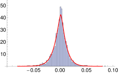
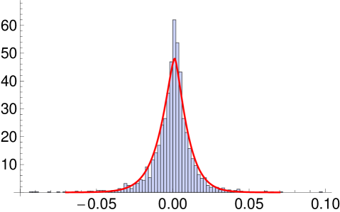
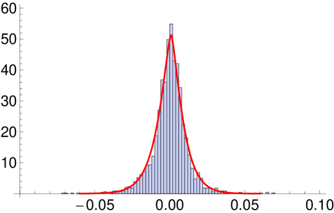
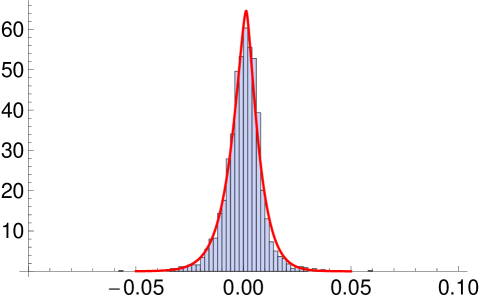
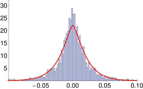
The two sets of model parameters are not directly comparable. However the estimates of $\bm{\Sigma}$ and correlation matrices are very similar while $\bm{\gamma}$ are some what similar. The standard error for the estimate $\bm{\beta}_{1}$ in MSVG AR model suggests that only the second column has all parameters being significant. Since the second column of the $\bm{\beta}_{1}$ matrix has relatively larger values, all five stocks are strongly lag-one cross-correlated with S&P 500. It is not surprising to know that the returns in S&P 500 has the most impact on each of the five returns the next day because S&P 500 has been shown to be a strong predictor for a number of market indices. This is due to its large market share and its minimal real time difference with lag-one return of other markets. Comparing the AICc of the two models, the MSVG AR model provides better model fit which is further illustrated in the histogram of residuals in Figure 3 after filtering out the AR(1) term. Fitted marginal pdfs with $\bm{\beta}_{0}$ as the mean of the MSVG model are added to the figure to facilitate comparison. Overall the two MSVG models provide good fits to the data despite occasionally, the peaks of the histogram and fitted pdf around the means does not match exactly possibly due to the rather strong assumption of a common shape parameter $\nu$ across all components. This is a limitation of the MSVG distribution.

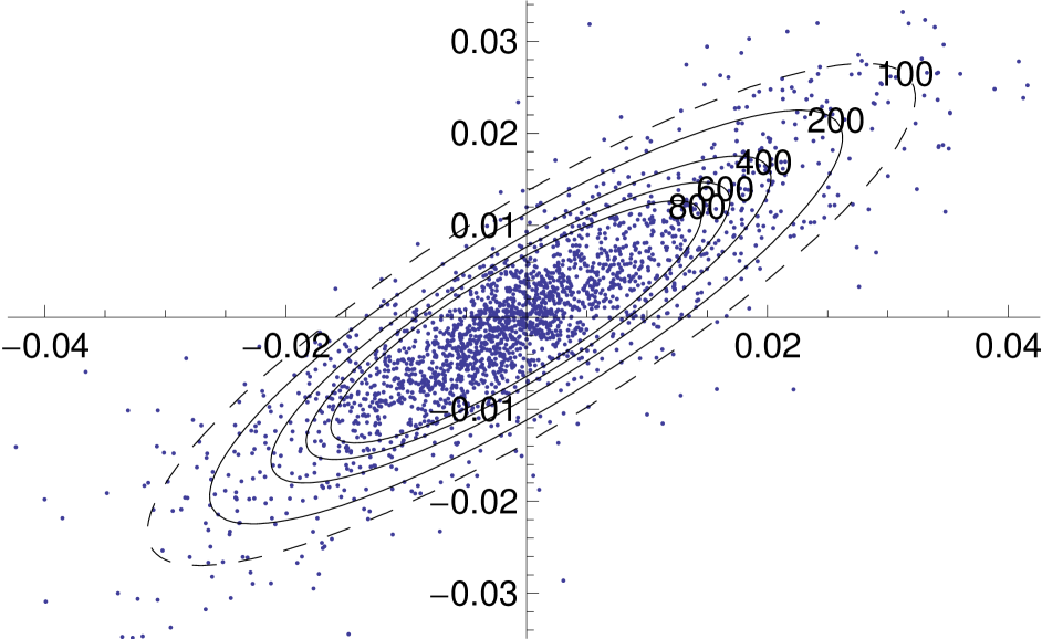
From the correlation matrices of the two models, the pair of market indices DAX and FTSE 100 are highly correlation ( $\rho_{13}\simeq 0.85$ ), possibly due to the strong competitiveness of the German and UK markets as they are the major stock markets in Europe. This gives rise to similar cross-correlation for both DAX and FTSE 100 with the other stocks. The model fit of the MSVG AR model for DAX and FTSE 100 bivariate return data is displayed in the contour plot in Figure 4. Since the parameter estimates are quite similar to the five dimensional empirical study, we omit reporting these results. Overall the model captures the strong correlation between the two stocks, giving a good overall fit to the DAX and FTSE 100 data set.

6 Conclusion

The MCECM and ECME algorithms have been proposed to obtain the ML estimates of multivariate Student-t distribution (Liu and Rubin,, 1995). We advance the algorithms to HECM algorithm and demonstrate its applicability to the MSVG model with AR mean function. Our proposed HECM algorithm with two adjustments solves three technical issues in application.

Firstly, HECM algorithm improves the overall computational efficiency by combining the speed of MCECM algorithm at the start of iterations with the stability of ECME algorithm at latter iterations. Secondly, when the shape parameter is small and observations cluster closely to the mean, the problem of unbounded MSVG density leading to diverged estimates $\widehat{1/\lambda_{i}}$ and $\widehat{\log\lambda_{i}}$ can be resolved by capping the density within certain range of $\Delta$ . We study the optimal choices of $\Delta$ ranges for dimension $d=2,3$ . More studies are needed to verify the choices of $\Delta$ for higher dimensions. Lastly, we add an extra E-step after updating $(\bm{\mu}^{(t+1)},\bm{\gamma}^{(t+1)})$ but before updating $\bm{\Sigma}^{(t+1)}$ to improve the stability of the $\hat{\bm{\Sigma}}$ estimate when the MSVG density is again unbounded.

The HECM algorithm is then applied to fit the MSVG model with an AR(1) mean structure to describe the dynamics in financial time series. To improve the model flexibility and predictability, the HECM algorithm can be easily extended to models with AR( $p$ ) terms. Moreover, the algorithm can be further enhanced to popular financial time series models such as GARCH models (Bollerslev,, 1986) and with leverage effect (Engle and Ng,, 1993). Some distribution families such as the multivariate skew Student-t distribution or multivariate skew generalised hyperbolic distribution which nests the MSVG distribution may be considered because they can be expressed in normal mean-variance mixtures representation. While these extensions improve the applicability of the algorithm, it is very challenging as there is no close-form solution for parameters in the mean function and hence more layers of iterations are required.

In summary, we show that the HECM algorithm improves the computation efficiency in the ML estimation for the complicated MSVG distribution in normal mean-variance mixtures representation. However, we also remark the limitation of the MSVG model with one shape parameter for all components. In practice, different time series may follow distributions with different shape parameters. Hence, to improve the model applicability, it is necessary to allow one shape parameter for each component resulting in a modified MSVG model, similar to the GARCH models in Choy et al., (2014).

Acknowledgments

I would like to thank John Ormerod for his helpful comments which leads to improvement of the paper.

References

Bollerslev, (1986) Bollerslev, T. (1986). Generalized autoregressive conditional heteroskedasticity. J. Econometrics, 31(3):307–327.
Choy and Smith, (1997) Choy, S. and Smith, A. (1997). Hierarchical models with scale mixtures of normal distributions. Test, 6(1):205–221.
Choy et al., (2014) Choy, S. T. B., Chen, C. W. S., and Lin, E. M. H. (2014). Bivariate asymmetric garch models with heavy tails and dynamic conditional correlations. Quantitative Finance, 14(7):1297–1313.
Dempster et al., (1977) Dempster, A. P., Laird, N. M., and Rubin, D. B. (1977). Maximum likelihood from incomplete data via the EM algorithm. J. Roy. Statist. Soc. Ser. B, 39(1):1–38. With discussion.
Embrechts, (1983) Embrechts, P. (1983). A property of the generalized inverse Gaussian distribution with some applications. J. Appl. Probab., 20(3):537–544.
Engle and Ng, (1993) Engle, R. F. and Ng, V. K. (1993). Measuring and testing the impact of news on volatility. J. Finance, 48(5):1749–1778.
Finlay and Seneta, (2008) Finlay, R. and Seneta, E. (2008). Stationary-increment variance-gamma and ”t” models: Simulation and parameter estimation. Int. Statist. Rev., 76(2):167–186.
Fung and Seneta, (2007) Fung, T. and Seneta, E. (2007). Tailweight, quantiles and kurtosis: a study of competing distributions. Oper. Res. Lett., 35(4):448–454.
Fung and Seneta, (2010) Fung, T. and Seneta, E. (2010). Modelling and estimation for bivariate financial returns. Int. Statist. Rev., 78(1):117–133.
Gradshteyn and Ryzhik, (2007) Gradshteyn, I. S. and Ryzhik, I. M. (2007). Table of integrals, series, and products. Elsevier/Academic Press, Amsterdam, seventh edition. Translated from the Russian, Translation edited and with a preface by Alan Jeffrey and Daniel Zwillinger, With one CD-ROM (Windows, Macintosh and UNIX).
Hu and Kercheval, (2008) Hu, W. and Kercheval, A. N. (2008). The skewed $t$ distribution for portfolio credit risk. In Econometrics and risk management, volume 22 of Adv. Econom., pages 55–83. Emerald/JAI, Bingley.
Liu and Rubin, (1994) Liu, C. and Rubin, D. B. (1994). The ECME algorithm: a simple extension of EM and ECM with faster monotone convergence. Biometrika, 81(4):633–648.
Liu and Rubin, (1995) Liu, C. and Rubin, D. B. (1995). ML estimation of the $t$ distribution using EM and its extensions, ECM and ECME. Statist. Sinica, 5(1):19–39.
Louis, (1982) Louis, T. A. (1982). Finding the observed information matrix when using the EM algorithm. J. Roy. Statist. Soc. Ser. B, 44(2):226–233.
Madan and Seneta, (1987) Madan, D. B. and Seneta, E. (1987). Chebyshev polynomial approximations and characteristic function estimation. J. Roy. Statist. Soc. Ser. B, 49(2):163–169.
Madan and Seneta, (1990) Madan, D. B. and Seneta, E. (1990). The variance gamma (V.G.) model for share market returns. J. Bus., 63(4):511–524.
McNeil et al., (2005) McNeil, A. J., Frey, R., and Embrechts, P. (2005). Quantitative risk management. Princeton Series in Finance. Princeton University Press, Princeton, NJ. Concepts, techniques and tools.
Meng, (1994) Meng, X.-L. (1994). On the rate of convergence of the ECM algorithm. Ann. Statist., 22(1):326–339.
Meng and Rubin, (1993) Meng, X.-L. and Rubin, D. B. (1993). Maximum likelihood estimation via the ECM algorithm: a general framework. Biometrika, 80(2):267–278.
Tjetjep and Seneta, (2006) Tjetjep, A. and Seneta, E. (2006). Skewed normal variance-mean models for asset pricing and the method of moments. Int. Statist. Rev., 74(1):109–126.