An Efficient Approach for Computing Optimal Low-Rank Regularized Inverse Matrices
Abstract
Standard regularization methods that are used to compute solutions to ill-posed inverse problems require knowledge of the forward model. In many real-life applications, the forward model is not known, but training data is readily available. In this paper, we develop a new framework that uses training data, as a substitute for knowledge of the forward model, to compute an optimal low-rank regularized inverse matrix directly, allowing for very fast computation of a regularized solution. We consider a statistical framework based on Bayes and empirical Bayes risk minimization to analyze theoretical properties of the problem. We propose an efficient rank update approach for computing an optimal low-rank regularized inverse matrix for various error measures. Numerical experiments demonstrate the benefits and potential applications of our approach to problems in signal and image processing.
Keywords: ill-posed inverse problems, regularization, low-rank approximation, TSVD, Bayes risk, empirical Bayes risk, machine learning
1 Introduction
Inverse problems arise in scientific applications such as biomedical imaging, geophysics, computational biology, computer graphics, and security [1, 2, 3, 4, 5, 6, 7, 8]. Assume that and are given, then the linear inverse problem can be written as
| (1) |
where is the desired solution and is additive noise. We assume the underlying problem is ill-posed. A problem is ill-posed if the solution does not exist, is not unique, or does not depend continuously on the data [9]. A main challenge of ill-posed inverse problems is that small errors in the data may result in large errors in the reconstruction. In order to obtain a more meaningful reconstruction, regularization in the form of prior knowledge is needed to stabilize the inversion process.
Standard regularization methods require knowledge of [10, 2]. However, in many applications, the operator may not be readily available, or is only partially known. In this work, we investigate an approach that avoids including in the problem formulation, and instead learns the necessary information from training or calibration data. Assume training data for , for (1) are given. First, our goal is to find a rank- matrix that gives a small error for the given training set. That is, the sample mean error,
| (2) |
should be small for some given error measure , e.g., . Here, refers to the sample error for a single observation . In this paper, we consider efficient methods for obtaining an optimal low-rank regularized inverse matrix,
| (3) |
Then, once matrix is computed, solving the inverse problem (1) requires a simple matrix-vector multiplication: . Matrix can be precomputed, so that regularized solutions to inverse problems can be obtained efficiently and accurately.
Methods that incorporate training data have been widely used in machine learning [11, 12] and have been analyzed in the statistical learning literature [13]. Most previous work on using training data for solving inverse problems has been restricted to minimizing the predictive mean squared error and require knowledge of the forward model [14, 15]. In this paper, we provide a novel framework to solve inverse problems that does not require knowledge of the forward model. We develop efficient methods to compute an optimal low-rank regularized inverse matrix for a variety of error measures. In addition, we provide a natural framework for evaluating solutions and predicting uncertainties.
The paper is structured as follows. In Section 2 we provide background on regularization of inverse problems and discuss the connection to Bayes risk minimization. Some theoretical results are provided for the corresponding Bayes risk minimization problem. In Section 3 we describe numerical methods to efficiently solve (3), including a rank-update approach that can be used for various error measures and large-scale problems. Numerical results are presented in Section 4 and conclusions are provided in Section 5.
2 Background and Motivation
The singular value decomposition (SVD) is an important tool for analyzing regularization methods. For any real matrix , let be the SVD, where is a diagonal matrix containing the singular values, and orthogonal matrices and contain the left and right singular vectors and respectively [16]. For a given positive integer , define
where , and
Then, we denote to be the pseudoinverse of [17].
For ill-posed inverse problems, the singular values of decay to and cluster at zero. Spectral filtering methods provide solutions where components of the solution corresponding to the small singular values are damped or neglected. For example, the rank- truncated SVD (TSVD) solution can be written as
| (4) |
In Figure 1, we provide TSVD sample mean errors for different values of for a image deblurring problem. For TSVD, the choice of rank is crucial. For small rank, there are not enough singular vectors to capture the details of the solution, but for large rank, small singular values are included, and noise corrupts the solution. This is an illustrative example, so details are not specified here. See Section 4 for more thorough numerical investigations.
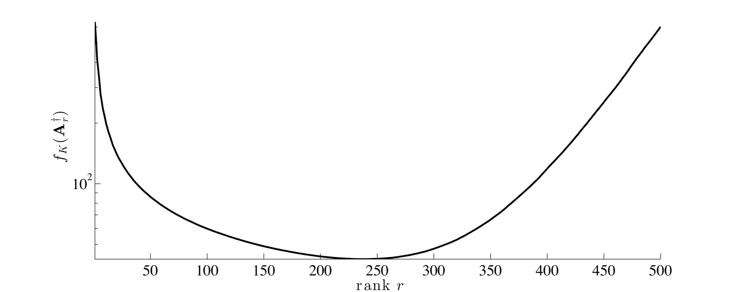
It is worth noting that the TSVD reconstruction matrix is one example of a rank- matrix that solves (1). In this paper, we seek an optimal rank- matrix for all training data. Computing a solution to problem (3) is non-trivial, and in the next section we provide some underlying theory from a Bayes risk perspective.
2.1 Bayes risk minimization
By interpreting problem (3) as an empirical Bayes risk minimization problem [18, 13, 19], we can provide a statistical framework for analyzing the problem and motivate numerical algorithms for computing an optimal low-rank regularized inverse matrix. In the following we assume that and are random variables with given probability distributions and . Using the fact that , the Bayes risk minimization problem can be written as,
| (5) |
where is the expected value with respect to the joint distribution of and [18, 13]. The particular choices of and in (5) determine an optimal reconstruction matrix . Optimization problem (3) can be interpreted as an empirical Bayes risk minimization problem corresponding to Bayes risk minimization problem (5), where and denote realizations of the random variables and .
2.2 Bayes Risk Minimization for the 2-norm case
For the special case where the Bayes risk can be written as
| (6) |
In this section, we provide closed form solutions for both the unconstrained and rank-constrained Bayes risk minimization problems for the 2-norm case.
We assume that the random variables and are statistically independent. Let be the mean and be the covariance matrix for the distribution . Similarly, and are the mean and covariance matrix for . We assume that both matrices are positive definite and that all entries are finite. One fact that will be useful to us is that the expectation of the quadratic form involving a symmetric matrix and a random variable with covariance matrix can be written as
where denotes the trace of a matrix [20]. With this framework and the Cholesky decompositions and , we can write the Bayes risk (6) as,
where denotes the Frobenius norm of a matrix.
We can simplify this final expression by pre-whitening the noise , thereby converting to a coordinate system where the noise mean is zero and the noise covariance is a multiple of the identity. Define the random variable
| (7) |
Then, and and we have
| (8) |
which can be written as,
| (9) |
where and Thus, without loss of generality (although with the need for numerical care if is ill-conditioned), we can always assume that and . Therefore, our Bayes risk (6) takes the form
| (10) |
Under certain conditions, summarized in the following theorem, there exists a unique global minimizer for (10).
Theorem 2.1.
Given , , and , consider the problem of finding a matrix with
| (11) |
If either or if has rank and is nonsingular, then the unique global minimizer is
| (12) |
Proof.
Using derivatives of norms and traces, we get
| (13) |
Setting the above derivative equal to zero gives the following first order condition,
| (14) |
Under our assumptions, the matrix is invertible, so we get the unique solution that is given in the statement of the Theorem. It is a minimizer since the second derivative matrix of is positive definite. ∎
To summarize, we have minimized the Bayes risk (6) under the assumptions that and are statistically independent random variables with symmetric positive definite finite covariance matrices.
Next we consider the rank-constrained Bayes risk minimization problem. With the additional assumption that , problem (5) can be written as
| (15) |
where and A closed form solution to (15) was recently provided in [21], and the result is summarized in the following theorem.
Theorem 2.2.
Given a matrix where and an invertible matrix , let their generalized singular value decomposition be , . Let be a given parameter, nonzero if . Let be a given positive integer. Define . Let the symmetric matrix have eigenvalue decomposition with eigenvalues ordered so that for . Then a global minimizer of problem (15) is
| (16) |
where contains the first columns of . Moreover this is the unique global minimizer of (15) if and only if .
Next we consider the case where for some scalar . In this case the Bayes risk simplifies to
| (17) |
and, by rescaling, the low-rank Bayes risk minimization problem can be restated as optimization problem (15) where represents the noise-to-signal ratio and . It was shown in [21] that for this problem, the global minimizer simplifies to
| (18) |
where and and were defined in the beginning of this section. Moreover, is the unique global minimizer if and only if . For problems where is known, matrix can be used to compute a filtered solution to inverse problems. That is,
where the filter factors are given by
Here, is the truncated Tikhonov reconstruction matrix [21].
3 Computing Low-rank Regularized Inverse Matrices
In this section, we describe numerical methods to efficiently compute a low-rank regularized inverse matrix, i.e., a solution to (3), for problems where matrix is unknown and training data are available. We first describe a method that can be used for the special case where . Further we discuss a rank-update approach that can be utilized for large-scale problems and for general error measures.
3.1 2-norm case
For the case , we can use the relationship between the 2-norm of a vector and the Frobenius norm of a matrix to rewrite optimization problem (3) as
| (19) |
where and . A closed form solution for (19) exists, and the result is summarized in the following theorem.
Theorem 3.1.
Let matrices and be given. Further let be the matrix of right singular vectors of and define where . Then
is a solution to the minimization problem (19). This solution is unique if and only if either or and , where and denote the and st singular values of .
Proof.
The main computational cost of constructing using Theorem 3.1 lies in two SVD computations (for matrices and ). If these computations are possible and minimizing the mean squared error is desired, then we propose to use the above result to compute optimal low-rank regularized inverse matrix , which in turn can be used to solve inverse problems [24].
3.2 A rank-update approach
For general error measures or for large problems with large training sets, we propose a rank-update approach for obtaining optimal low-rank regularized inverse matrix . The approach is motivated by the following corollary to Theorem 2.2.
Corollary.
Corollary Corollary states that in the Bayes framework for the 2-norm case, a rank-update approach (in exact arithmetic) can be used to compute an optimal low-rank regularized matrix. That is, assume we are given the rank- approximation and we are interested in finding . To calculate the optimal rank- approximation , we just need to solve a rank- optimization problem of the form (20) and then update the solution, .
We are interested in the empirical Bayes problem, and we extend the rank-update approach to problem (3), where the basic idea is to iteratively build up matrices and such that Suppose we are given the optimal rank- matrix . That is, solves (3) for . Then, we compute a rank- update to by solving the following rank- optimization problem,
| (21) |
and a rank- regularized inverse matrix can be computed as . This process continues until the desired rank is achieved. A summary of the general algorithm can be found below, see Algorithm 1.
Next we provide some computational remarks for Algorithm 1.
Choice of .
At each iteration of Algorithm 1, we must solve optimization problem (21), which has unknowns. Hence, the choice of will depend on the size of the problem and may even vary per iteration, e.g., . For large-scale problems such as those arising in image reconstruction, we recommend updates of size to keep optimization problem (21) as small as possible.
Stopping criteria.
Stopping criteria for Algorithm 1 should have four components. First, a safe-guard maximal rank condition. That is, we stop if is greater than some pre-determined integer value . Secondly, let be a user-defined error tolerance for the function value, then we stop if . Similarly, we can monitor the relative improvement of in each iteration and stop if the relative improvement is smaller than some tolerance. Lastly, if a rank- update does not substantially improve , the iteration should be terminated. More specifically, let and choose tolerance . Then we can control the rank deficiency of by stopping if . The particular choices of stopping criteria and tolerances are problem dependent.
Solving rank- update problem (21).
The main challenge for Algorithm 1 is in line 3, where we need to solve the rank- update problem (21). First, we remark that the solution is not unique. In fact, for any . As a consequence optimization problem (21) is ill-posed and a particular solution needs to be selected. Various computational approaches exist to handle this kind of ill-posedness. One way to tackle this problem is to constrain each column in to have norm , i.e., for , and solve the constrained or relaxed joint optimization problem. We found this approach to be computationally inefficient and instead propose an alternating optimization approach. Notice that for any convex function , function is convex in and convex in , so an alternating optimization approach avoids the above ill-posedness. Until convergence, the solution to is computed for fixed , and then the solution to is computed for fixed . Columns of are normalized at each iteration. The alternating optimization is summarized in Algorithm 2.
Methods for solving optimization problems in lines 3 and 4 of Algorithm 2 depend on the specific form of . For instance for with we suggest using Gauss-Newton type methods. For -norms with we propose to use Quasi-Newton type methods such as SR1, BFGS, and LBFGS [25] or utilize smoothing techniques to compensate for discontinuities in the derivative. Standard stopping criteria can be used for these optimization problems, as well as for Algorithm 2 [26]. The required gradients of and Gauss-Newton approximation to the Hessian are provided below.
Let , , and . Then the gradients are given by
| (22) |
where with evaluated at . The Jacobian matrices have the form,
where and . The Gauss-Newton approximations of the Hessians are given by
| (23) |
where and evaluated at . Note that is diagonal for any error measures of the form which includes the Huber function and all -norms with .
Another important remark is that for computational efficiency, we do not need to form explicitly. That is, if we let then (21) can be reformulated as
| (24) |
where vectors should be updated at each iteration as
Using to solve inverse problems.
We have described some numerical approaches for computing , and it is worthwhile to note that all of these computations can be done off-line. Once computed, the optimal low-rank regularized inverse matrix can be used to solve inverse problems very quickly, requiring only one matrix-vector multiplication , if is obtained explicitly, or two multiplications if and are computed separately. This is particularly important for applications where hundreds of inverse problems need to be solved in real time. The ability to obtain fast and accurate reconstructions of many inverse problems in real time quickly compensates for the initial cost of constructing (or and ).
One of the significant advantages of our approach is that we seek a regularized inverse matrix directly, so that knowledge of the forward model is not required. However, for applications where is desired, our framework could be equivalently used to first estimate a low-rank matrix from the training data by solving Equation (3) where is and and are switched. This approach is similar to ideas from machine learning [27, 28] and are related to matrix completion problems where the goal is to reconstruct unknown or missing values in the forward matrix [29]. Then, once is computed, standard regularization methods may be required to solve inverse problems. If this is the case, we propose to use the training data to obtain optimal regularization parameters, as discussed in [14]. Since the ultimate goal in many applications is to compute solutions to inverse problems, obtaining an approximation of is not necessary and may even introduce additional errors. Thus, if is not required, our approach to compute the optimal regularized inverse matrix is more efficient and less prone to errors.
4 Numerical Results
In this section, we compute optimal low-rank regularized inverse matrices for a variety of problems and evaluate the performance of these matrices when solving inverse problems. We generated a training set of observations, and . Then for various error measures, , we compute optimal low-rank regularized inverse matrices as described in Section 3. To validate the performance of the computed optimal low-rank regularized inverse matrices, we generate a validation set of different observations, and compute the error between the reconstructed solution and the true solution , i.e., . For each experiment, we report the sample mean error as computed in (2), along with other descriptive statistics regarding the error distributions.
Standard regularization methods such as TSVD require knowledge of , while our approach requires training data. Thus, it is difficult to provide a fair comparison of methods. In our experiments, we compare our reconstructions to two “standard” reconstructions:
-
•
TSVD-: This refers to the TSVD reconstruction, as computed in (4), and it requires matrix and its SVD. The rank- reconstruction matrix for TSVD- is given by
-
•
TSVD-: If is not available, one could estimate it from the training data by solving the following rank-constrained optimization problem,
(25) for some fixed integer We propose to use methods described in Section 3 to obtain matrix . Then, the computed matrix could be used to construct a TSVD reconstruction. We refer to this approach as TSVD-, and the rank- reconstruction matrix for TSVD- for is given by This seems to be a fair comparison to our approach since only training data is used; however, a potential disadvantage of TSVD- is that can be large, and computing its SVD may be prohibitive.
We present results for three experiments: Experiments 1 and 2 are 1D examples, and Experiment 3 is a 2D example.
4.1 One-dimensional examples
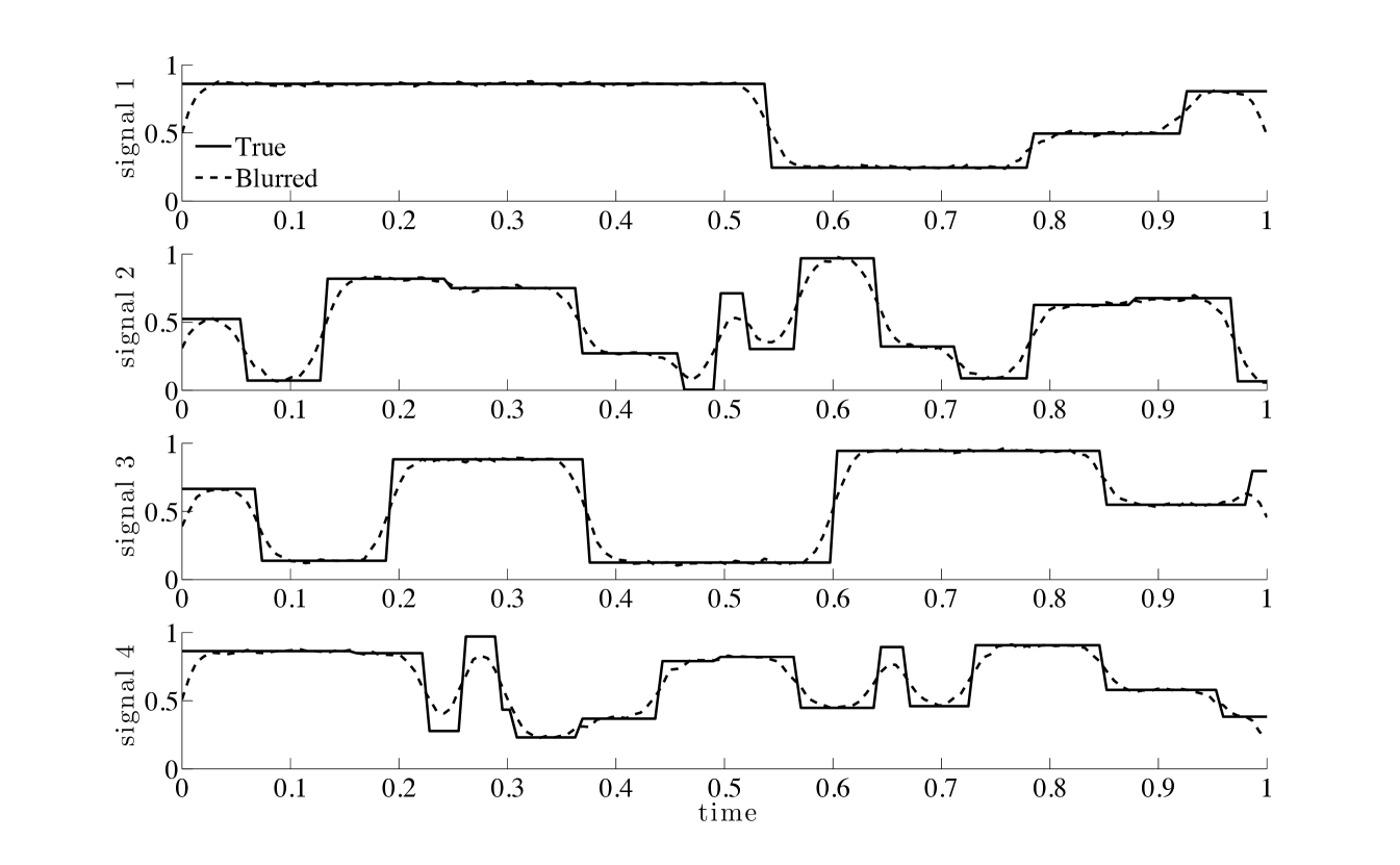
For the 1D examples, we use random time signals by generating piecewise constant functions as seen in Figure 2. Here, the number of jumps in each signal is a randomly chosen integer between 3 and 20, drawn from a uniform distribution. The times for the jumps and the signal strength were both randomly selected in the interval , also from a uniform distribution. The discretized signal has length The corresponding blurred signals were computed as in Equation (1), where matrix is and represents convolution with a 1D Gaussian kernel with zero mean and variance 2, and represents Gaussian white noise. The noise level for the blurred signals was , which means that . Training and validation signals were generated in the same manner. Figure 2 displays four sample signals from the validation set and their corresponding observed signals.
Experiment 1.
For this experiment, we consider the case where and compute an optimal regularized inverse matrix (ORIM) as described in Section 3.1. We refer to this approach as and we refer to the computed matrix as .
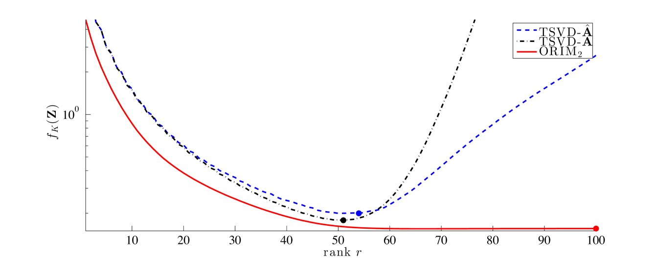
First, we fix the number of training signals to . For varying ranks we compute the sample mean error for , TSVD-, and TSVD- for a set of different validation signals. For computing , was fixed to . Errors plots as a function of rank are shown in Figure 3. We observe that the sample mean error for ORIM2 is monotonically decreasing and consistently smaller than the sample mean errors for both TSVD- and TSVD-. This is true for all ranks. Furthermore, both TSVD- and TSVD- exhibit semi-convergence behavior similar to Figure 1, whereby the error initially improves as the rank increases, but reconstructions degrade for larger ranks. On the other hand, since regularization is built into the design and construction of , avoids semi-convergence behavior altogether, as evident in the flattening of the error curve. Thus, solutions are less sensitive to the choice of rank.
For ranks less than , TSVD- achieves a smaller sample mean error than TSVD-. We also note that the smallest error that TSVD- can achieve is larger than the smallest error than TSVD- can achieve. This is to be expected since is an approximation of Although the semi-convergence phenomenon for TSVD- occurs later and errors grow slower than for TSVD-, both TSVD solutions require the selection of a good choice for the rank. Since training data is available, one could use the training data to select an “optimal” rank for TSVD- and TSVD-, i.e., the rank which provides the minimal sample mean error for the training set. This is equivalent to the opt-TSVD approach from [14]. For TSVD- and TSVD-, the minimal sample mean error for the training set occurs at ranks 51 and 54 (consistent with validation set), respectively.
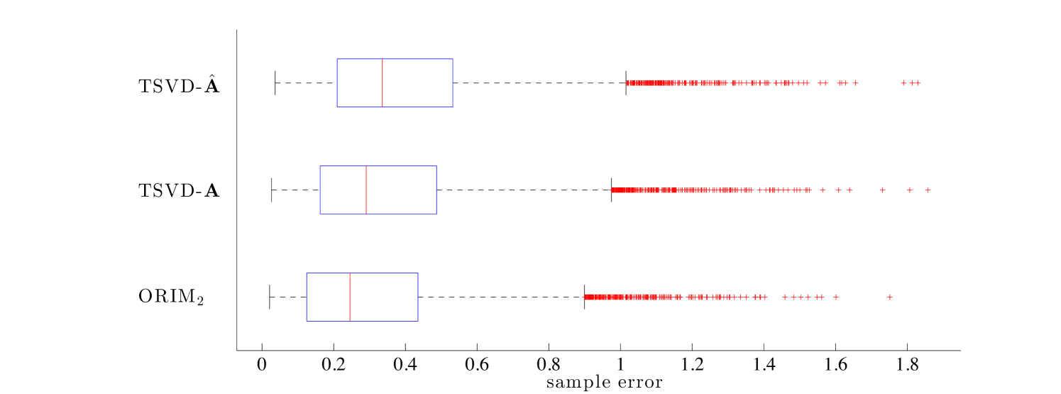
In Figure 4, we provide box-and-whisker plots to describe the statistics of the sample errors for the validation set, for . Each box provides the median error, along with the 25th and 75th percentiles. The whiskers include extreme data, and outliers are plotted individually. For TSVD- and TSVD-, errors correspond to the ranks computed using the opt-TSVD approach ( = 51 and 54 respectively), and errors for correspond to maximal rank 100. The average of the errors correspond to the dots in Figure 3.
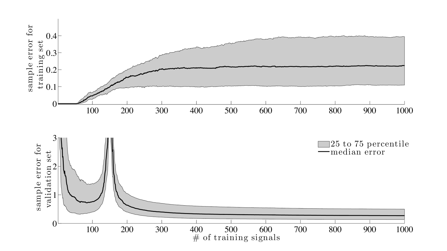
Next, we investigate how the errors for ORIM2 vary for different numbers of training signals. That is, for increasing numbers of training signals, we compute the matrix and record sample errors for both the training set and the validation set. It is worthwhile to mention that the rank of is inherently limited by the number of training signals and the signal length, i.e., . For this example, we have and we select the rank of to be
| (26) |
Notice that for rank with a signal length of , we have a total of unknowns (for and ). In Figure 5 we provide the median errors along with the 25th to 75th percentiles. These plots are often referred to as Pareto curves in the literature.
We observe that for the number of training signals the ORIM2 matrix is significantly biased towards the training set. This is evident in the numerically zero computed errors for the training set. In addition, we expect the errors for the training set to increase and the errors for the validation set to decrease as more training signals are included in the training set, due to a reduction in bias towards the training set. Eventually, errors for both signal sets reach a plateau, where additional training data do not significantly improve the solution. The point at which the errors begin to stabilize indicates a natural choice for the number of training signals to use, e.g., when the relative change in errors reaches a predetermined tolerance. For this example a relative improvement of for the errors for the training set is reached at training images.
There is an interesting phenomena that occurs in the reconstruction errors for the validation set, whereby the error peaks around . Although puzzling at first, the peak in errors is intuitive when one considers the problem that is being solved. For matrix is If is full rank (), in Theorem 3.1 and problem (19) has the solution,
which is the special case considered by Eckart-Young and Schmidt [30, 31] Notice that is uniquely determined by the training set, so reconstructions at this point will be most biased to the training set.
Experiment 2.
For this experiment, we use the same setup as described in Experiment 1 for the 1D example, but we compare results obtained by using different error measures in equation (3). In particular, we consider for and For we use additional smoothing to deal with non-differentiability. We compute an optimal low-rank regularized inverse matrix for each . The computed matrices are then used to reconstruct the validation set. We refer to these approaches as and , respectively. Box-and-whisker plots of the sample errors for the validation signals are presented in Figure 6, along with errors for TSVD-. In each subfigure, the reconstruction error was computed using a different error measure. As expected, the reconstructions with smallest error correspond to where defines the error measure used for the training set.
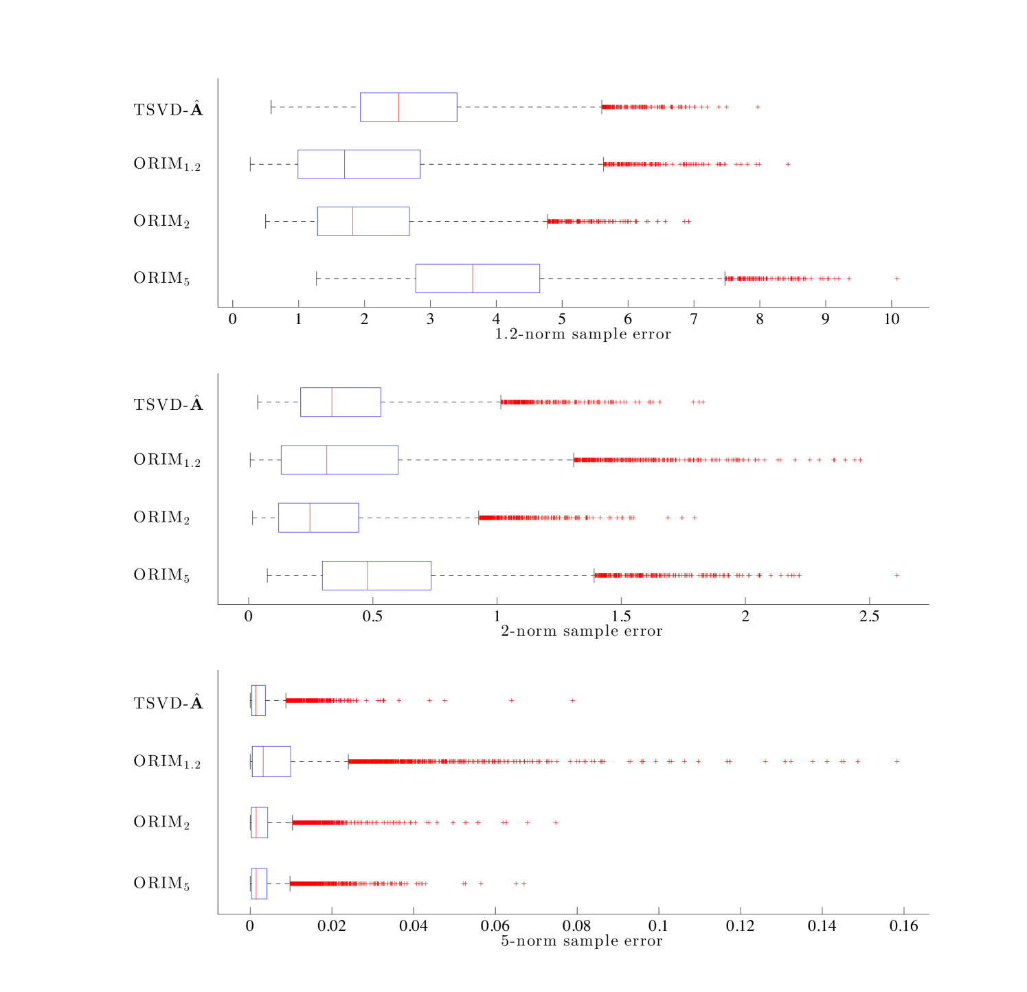
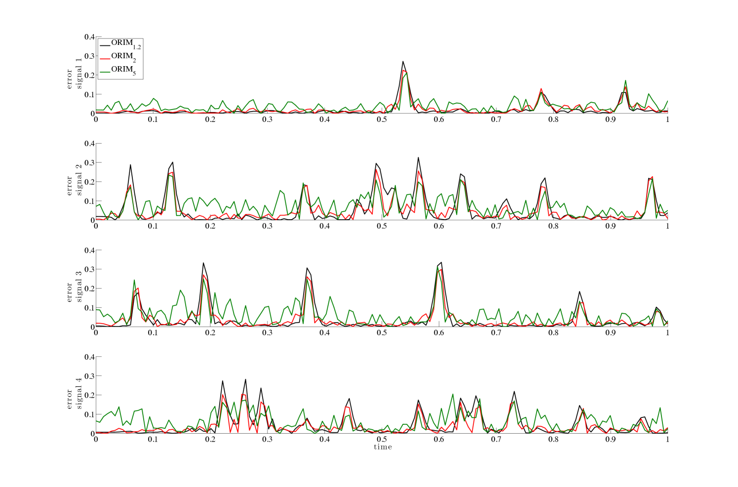
We emphasize that even though the sample errors for the various methods may appear similar in value in the box plots, the reconstructions are significantly different, as seen in the absolute errors. Plots of the absolute values of the error vectors, for the four validation signals presented in Figure 2 can be found in Figure 7. We observe that allows for large reconstruction errors throughout the signal without major peaks, while absolute reconstruction errors for tend to remain small in flat regions, with only a few high peaks in the error at locations corresponding to discontinuities in the signal. These observations are consistent with norms in general and illustrate the potential benefits of using a different error measure.
4.2 Two-dimensional example
Next, we describe a problem from image deblurring, where the underlying model can be represented as (1) where matrix represents a blurring process, and and represent the true and observed images respectively. Entries in matrix depend on the point spread function (PSF). For image deblurring examples, matrix is typically very large and sparse. However, under assumptions of spatial invariance and assumed boundary conditions and/or properties of the PSF, structure in can be exploited and fast transform algorithms can be used to efficiently diagonalize [5]. For example, if the PSF satisfies a double symmetry condition and reflexive boundary conditions on the image are assumed, then can be diagonalized using the 2D discrete cosine transform (DCT). Of course, these approaches rely on knowledge of the exact PSF.
Blind deconvolution methods have been developed for problems where the PSF is not known or partially known [32]; however, most of these approaches require strict assumptions on the PSF such as spatial invariance or parameterization of the blur function, or they require a good initial estimate of the PSF. Our approach uses training data and does not require knowledge of and, hence, knowledge of the PSF. Furthermore, we do not require any assumptions regarding spatial invariance of the blur, boundary conditions, or special properties of the blur (e.g., separability, symmetry, etc.). We refer the reader to [24] for comparisons to blind deconvolution methods.
Experiment 3.
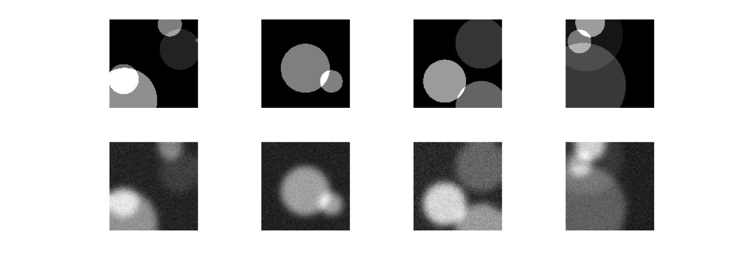
In this experiment, we generate a set of training images. Each image has pixels and represents a collection of circles, where the number of circles, location, radius and intensity were all randomly drawn from a uniform distribution. In this example, the PSF was a 2D Gaussian kernel with zero mean and variance 5. We assume reflexive boundary conditions for the image, and Gaussian white noise was added to each image, where the noise level was randomly selected between and . Sample true images along with the corresponding blurred, noisy image can be found in Figure 8. A validation set of images was generated in the same manner.
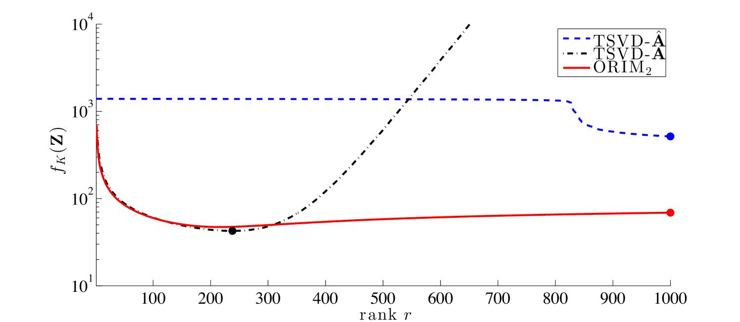
We compare the sample mean errors for the validation set for , TSVD-, and TSVD-, where the maximal rank for was . The sample mean errors are provided in Figure 9 for various ranks. Dots correspond to minimal sample mean error for the training data. As expected, TSVD- exhibits clear semi-convergence behavior, where the minimum error is achieved at rank (for both the training and validation sets). In contrast, ORIM2 maintains low sample mean errors for various ranks, and only exhibits slight semiconvergence for larger ranks. This can be attributed to bias towards the training data, since for larger ranks, more training data is required to compensate for more unknowns. We observe that the relative difference between the lowest sample mean error for ORIM2 and the lowest sample mean error for TSVD- is approximately . That is, even without knowledge of , ORIM2 can produce reconstructions that are comparable to TSVD- reconstructions.
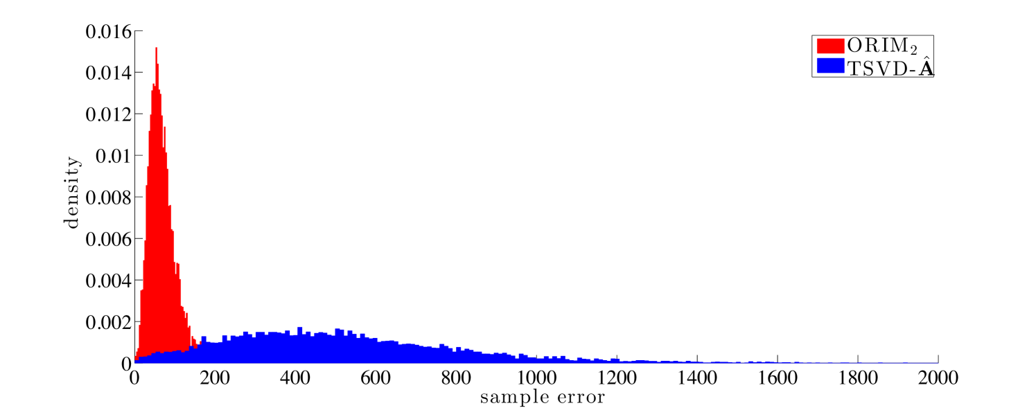
Next, we compare the distribution of the sample errors for ORIM2 and TSVD-, corresponding to rank Density plots can be found in Figure 10. Among the methods that only require training data, ORIM2 is less sensitive than TSVD-, implying that it is better to seek a low rank regularized inverse matrix directly, versus seeking a low rank approximation to and then inverting it.
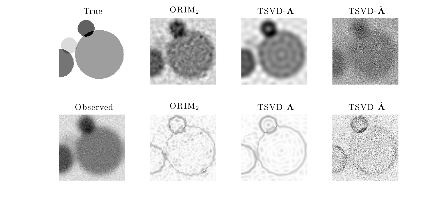
One of the validation images, with corresponding observed image can be found in the first column of Figure 11. Reconstructions for ORIM2, TSVD-, and TSVD-, and corresponding absolute error images between the reconstructed image and the true image (with inverted colormap so that white corresponds to zero error) are provided in Figure 11 (top and bottom row respectively).
5 Conclusions
In this paper, we described a new framework for solving inverse problems where the forward model is not known, but training data is readily available. We considered the problem of finding an optimal low-rank regularized inverse matrix that, once computed, can be used to solve hundreds of inverse problems in real time. We used a Bayes risk minimization framework to provide underlying theory for the problem. For the empirical Bayes problem, we proposed a rank- update approach and showed that this approach is optimal in the Bayes framework for the -norm. Numerical results demonstrate that our approach can produce solutions which are superior to standard methods like TSVD, but without full knowledge of the forward model. The examples illustrate the benefits of using different error measures and the potential for use in large-scale imaging applications.
Acknowledgment
We are grateful to Dianne P. O’Leary for helpful discussions.
References
- [1] H.W. Engl, M. Hanke, and A. Neubauer. Regularization of Inverse Problems. Springer, New York, 2000.
- [2] C.R. Vogel. Computational Methods for Inverse Problems. SIAM, Philadelphia, 2002.
- [3] A.G. Ramm. Inverse Problems: Mathematical and Analytical Techniques with Applications To Engineering. Springer, New York, 2004.
- [4] A. Tarantola. Inverse Problem Theory and Methods for Model Parameter Estimation. SIAM, Philadelphia, 2005.
- [5] P.C. Hansen, J.G. Nagy, and D.P. O’Leary. Deblurring Images: Matrices, Spectra and Filtering. SIAM, Philadelphia, 2006.
- [6] A. Kirsch. An Introduction to the Mathematical Theory of Inverse Problems. Springer, New York, 2011.
- [7] R.C. Aster, B. Borchers, and C.H. Thurber. Parameter Estimation and Inverse Problems. Academic Press, Waltham, 2012.
- [8] F.D.M. Neto and A.J.S. Neto. An Introduction to Inverse Problems With Applications. Springer, New York, 2012.
- [9] J. Hadamard. Lectures on Cauchy’s Problem in Linear Differential Equations. Yale University Press, New Haven, 1923.
- [10] P.C. Hansen. Rank-deficient and Discrete Ill-posed Problems. SIAM, Philadelphia, 1998.
- [11] M. Mohri, A. Rostamizadeh, and A. Talwalkar. Foundations of Machine Learning. The MIT Press, Cambridge, MA, 2012.
- [12] Y.S. Abu-Mostafa, M. Magdon-Ismail, and H.T. Lin. Learning from Data. AMLBook, 2012.
- [13] V.N. Vapnik. Statistical Learning Theory. Wiley, San Francisco, 1998.
- [14] J. Chung, M. Chung, and D.P. O’Leary. Designing optimal filters for ill-posed inverse problems. SIAM Journal on Scientific Computing, 33(6):3132–3152, 2011.
- [15] J. Chung, M. Chung, and D.P. O’Leary. Optimal filters from calibration data for image deconvolution with data acquisition error. Journal of Mathematical Imaging and Vision, 44(3):366–374, 2012.
- [16] G.H. Golub and C.F. Van Loan. Matrix Computations. Johns Hopkins University Press, Baltimore, 3 edition, 1996.
- [17] G.W. Stewart. Matrix Algorithms: Volume 1, Basic Decompositions. SIAM, Philadelphia, 1998.
- [18] B.P. Carlin and T.A. Louis. Bayes and Empirical Bayes Methods for Data Analysis. Chapman and Hall/CRC, Boca Raton, 2 edition, 2000.
- [19] A. Shapiro, D. Dentcheva, and R. Ruszczynski. Lectures on Stochastic Programming: Modeling and Theory. SIAM, Philadelphia, 2009.
- [20] G.A.F. Seber and A.J. Lee. Linear Regression Analysis. Wiley, San Francisco, 2 edition, 2003.
- [21] J. Chung, M. Chung, and D.P. O’Leary. Optimal regularized low rank inverse approximation. In revision at Linear Algebra and Applications, 2014.
- [22] D. Sondermann. Best approximate solutions to matrix equations under rank restrictions. Statistische Hefte, 27:57–66, 1986.
- [23] S. Friedland and A. Torokhti. Generalized rank-constrained matrix approximations. SIAM Journal on Matrix Analysis and Applications, 29(2):656–659, 2007.
- [24] J. Chung and M. Chung. Computing optimal low-rank matrix approximations for image processing. In IEEE Proceedings of the Asilomar Conference on Signals, Systems, and Computers. November 3-6, 2013, Pacific Grove, CA, USA, 2013.
- [25] J. Nocedal and S.J. Wright. Numerical Optimization. Springer, New York, 1999.
- [26] P.E. Gill, W. Murray, and M.H. Wright. Practical Optimization. Emerald Group Publishing, Bingley, UK, 1981.
- [27] P. Baldi and S. Brunak. Bioinformatics: the Machine Learning Approach. MIT press, Cambridge, 2001.
- [28] T. Hastie, R. Tibshirani, and J. Friedman. The Elements of Statistical Learning. Springer, New York, 2 edition, 2009.
- [29] J.-F. Cai, E. J. Candès, and Z. Shen. A singular value thresholding algorithm for matrix completion. SIAM Journal on Optimization, 20(4):1956–1982, 2010.
- [30] C. Eckart and G. Young. The approximation of one matrix by another of lower rank. Psychometrika, 1(3):211–218, 1936.
- [31] E. Schmidt. Zur Theorie der linearen und nichtlinearen Integralgleichungen. Mathematische Annalen, 63(4):433–476, 1907.
- [32] P. Campisi and K. Egiazarian. Blind Image Deconvolution: Theory and Applications. CRC press, Boca Raton, 2007.