An Efficient High-Dimensional Sparse Fourier Transform111This manuscript has been submitted to IEEE Transactions on Aerospace and Electronic Systems for reviewing on Sept. 1st, 2016.
Abstract
We propose RSFT, which is an extension of the one dimensional Sparse Fourier Transform algorithm to higher dimensions in a way that it can be applied to real, noisy data. The RSFT allows for off-grid frequencies. Furthermore, by incorporating Neyman-Pearson detection, the frequency detection stages in RSFT do not require knowledge of the exact sparsity of the signal and are more robust to noise. We analyze the asymptotic performance of RSFT, and study the computational complexity versus the worst case signal SNR tradeoff. We show that by choosing the proper parameters, the optimal tradeoff can be achieved. We discuss the application of RSFT on short range ubiquitous radar signal processing, and demonstrate its feasibility via simulations.
Index Terms:
Array signal processing, sparse Fourier transform, detection and estimation, radar signal processing.I Introduction
High dimensional FFT (N-D FFT) is used in many applications in which a multidimensional Discrete Fourier Transform (DFT) is needed, such as radar and imaging. However, its complexity increases with an increase in dimension, leading to costly hardware and low speed of system reaction. The recently developed Sparse Fourier Transform (SFT) [1, 2, 3, 4, 5, 6], designed for signals that have a small number of frequencies enjoys low complexity, and thus is ideally suited in big data scenarios [7, 8, 9]. One such application is radar target detection. The radar returns are typically sparse in the target space, i.e., the number of targets is far less than the number of resolutions cells. This observation motivates the application of SFT in radar signal processing.
The current literature on multi-dimensional extensions of the SFT include [10, 5, 3, 6]. Those works mainly address sample complexity, i.e., using the least number of time domain samples to reconstruct the signal frequencies. In order to detect the significant frequencies in an approximately sparse settings, i.e., signal corrupted by additive noise, the aforementioned methods assume knowing the exact sparsity, and compare the frequency amplitude with a predefined threshold. However, in many real applications, the exact signal sparsity may be either unknown or subject to change. For example, in the radar case, the number of targets to be detected is typically unknown and usually varies from time to time. Also, setting up an ideal threshold for detection in noisy cases is not trivial, since it relates to the tradeoff between probability of detection and false alarm rate. However, those issues have not been studied in the SFT literature.
One of the constrains in the aforementioned SFT algorithms is the assumption that the signal discrete frequencies are all on-grid. In reality, however, the signal frequencies, when discretized and depending on the grid size can fall between grid points. The consequence of off-grid frequencies is leakage to other frequency bins, which essentially reduces the sparsity of the signal. To refine the estimation of off-grid frequencies starting from the initial SFT-based estimates,[9] proposed a gradient descent method. However, the method of [9] has to enumerate all possible directions of the gradient for each frequency and compute the approximation error for each guessed direction, which increases the computational complexity. Moreover, like the other aforementioned SFT methods, the thresholding for frequency detection is not clear in [9]. The off-grid frequency problem in the context of SFT was also studied in [11], where it was assumed that in the frequency domain the signal and the noise are well separated by predefined gaps. However, this is a restrictive assumption that limits the applicability of the work.
In this paper we setup a SFT-based framework for sparse signal detection in a high dimensional frequency domain and propose a new algorithm, namely, the Realistic Sparse Fourier Transform (RSFT) which addresses the shortcomings discussed above. This paper makes the following contributions.
-
1.
The RSFT algorithm does not require knowledge of the number of frequencies to be estimated. Also, it does not need the frequencies to be on-grid and does not require signal and noise to be separated in the frequency domain. Our method reduces the leakage effect from off-grid frequencies by applying a window on the input time domain data (see Section III-A for details). The design of this window trades off frequency resolution, leakage suppression and computational efficiency. We shall point out that, unlike the work of [9] that recovers the exact off-grid frequency locations, our work aims to recover grided locations of off-grid frequencies with less amount of computation.
-
2.
We extend the RSFT into an arbitrary fixed high dimension, so that it can replace the N-D FFT in sparse settings and thus enable computational savings.
-
3.
We put RSFT into a Neyman-Pearson (NP) detection framework. Based on the signal model and other design specifications, we give the (asymptoticly) optimal thresholds for the two detection stages of the RSFT (see Section IV for details). Since the output of the first stage of detection serves as the input of the second stage, the two detection stages are interconnected. The detection thresholds are jointly found by formulating and solving an optimization problem, with its objective function minimizing the worst case Signal to Noise Ratio (SNR) (hence the system is more sensitive to weak signal), and its constrains connecting probability of detection and false alarm rate for both two stages.
-
4.
We provide a quantitive measure of tradeoff between computational complexity and worst case signal SNR for systems that use RSFT, which serves as a concrete design reference for system engineers.
-
5.
We investigate the use of RSFT in multi-dimensional radar signal processing.
A closely related technique to SFT is compressed sensing (CS). Compressed sensing-based methods recover signals by exploiting their sparse features [12]. The application of CS methods in MIMO radar is discussed intensively in [13, 14]. At a high level, CS differs from SFT in that it assumes the signal can be sparsely represented by an overdetermined dictionary, and formulates the problem as an optimization problem with sparsity constraints ( or norm). This problem is usually solved by convex optimization, which runs in polynomial time in for an -dimensional signal. On the other hand, the SFT method finds an (approximately) sparse Fourier representation of a signal in a mean square error sense ( norm). The sample and the computational complexity of SFT is sub-linear to , for a wide range of -dimensional signals [6].
A preliminary version of this work appeared in [15]. A detailed analysis of the RSFT algorithm as well as extensive experimental results are extensions to [15].
I-A Notation
We use lower-case (upper-case) bold letters to denote vectors (matrices). and respectively denote the transpose and conjugate transpose of a matrix or a vector. is Euclidean norm for a vector. is the element of vector . All operations on indices in this paper are taken modulo denoted by . We use to denote rounding to floor. refers to the set of indices , and is for eliminating element from set . We use to denote the set of -dimensional binary vectors. We use to denote forming a diagonal matrix from a vector and use to denote expectation. The DFT of signal is denoted as . We also assume that the signal length in each dimension is an integer power of 2.
This paper is organized as follows. A brief background on the SFT algorithm is given in Section II. Details of the proposed RSFT algorithm are given in Section III. Section IV presents the derivation of the optimal threshold design for the RSFT algorithm. Then in Section V we provide some numerical results to verify the theoretical findings. An application of the RSFT algorithm in radar signal processing is presented in Section VI and finally, concluding remarks are made in Section VII.
II Preliminaries
II-A Basic Techniques
As opposed to the FFT which computes the coefficients of all discrete frequency components of an -sample long signal, the SFT[2] computes only the frequency components of a -sparse signal. Before outlining the SFT algorithm we provide some key definitions and properties, which is extracted and reformulated based on [2] .
Definition 1.
(Permutation): Define the transform such that, given , and invertible
| (1) |
Then, the following transformation is called permutation
| (2) |
The permutation has the following property.
Property 1.
A modular reordering of the data in time domain results in a modular dilation and phase rotation in the frequency domain, i.e.,
| (3) |
Definition 2.
(Aliasing): Let , with powers of 2, and . For , a time-domain aliased version of x is defined as
| (4) |
Property 2.
Aliasing in time domain results in downsampling in frequency domain, i.e.,
| (5) |
Definition 3.
(Mapping): Let , where satisfies (1). We define the mapping such that
| (6) |
Definition 4.
II-B SFT Algorithm
At a high level, the SFT algorithm in [2] runs two loops, namely the Location loop and the Estimation loop. The former finds the indices of the most significant frequencies from the input signal, while the latter estimates the corresponding Fourier coefficients. Here, we emphasize on Location more than Estimation, since the former is more relevant to the radar application that we consider. The Location step provides frequency locations, which in the radar case is directly related to target parameters.
In the Location loop, a permutation procedure reorders the input data in the time domain, causing the frequencies to also reorder. The permutation causes closely spaced frequencies to appear in well separated locations with high probability. Then, a flat-window[2] is applied on the permuted signal for the purpose of extending a single frequency into a (nearly) boxcar, for a reason that will become apparent in the following. The windowed data are aliased, as in Definition 2. The frequency domain equivalent of this aliasing is undersampling by (see Property 2). The flat-window used at the previous step ensures that no peaks are lost due to the effective undersampling in the frequency domain. After this stage, a FFT of length is employed.
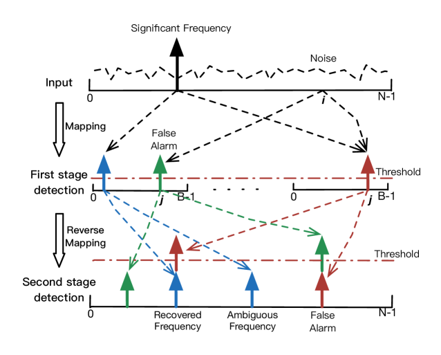
The permutation and the aliasing procedure effectively map the signal frequencies from -dimensional space into a reduced -dimensional space, where the first-stage-detection procedure finds the significant frequencies’ peaks, and then their indices are reverse mapped into the original -dimensional frequency space. However, the reverse mapping yields not only the true location of the significant frequencies, but also ambiguous locations for each frequency. To remove the ambiguity, multiple iterations of Location with randomized permutation are performed. Finally, the second-stage-detection procedure locates the most significant frequencies from the accumulated data for each iteration. More details about the SFT algorithm can be found in [2].
III The RSFT Algorithm
In this section we address some problems that have not been considered in the original SFT algorithm, namely the leakage from off-grid frequencies and optimal detection threshold design for both detection stages. Also, we extend the RSFT into arbitrary fixed high dimension.
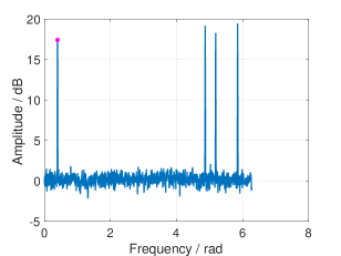
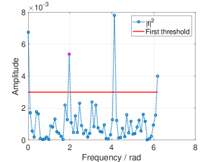
III-A Leakage Suppression for Off-grid Frequencies
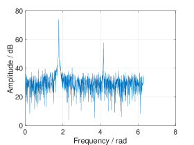
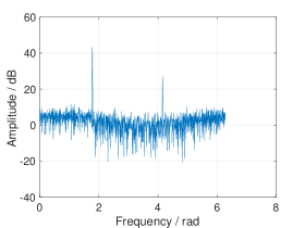
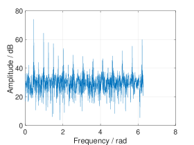
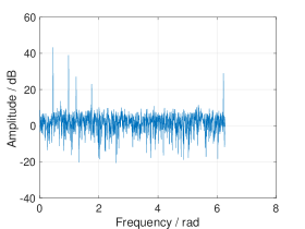
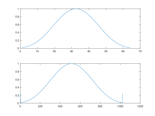
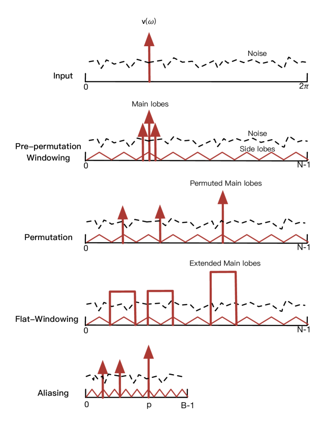
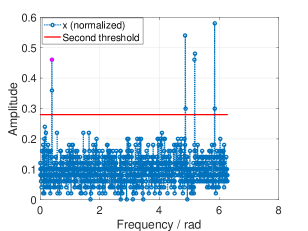
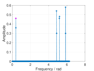
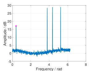
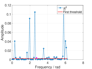
In real world applications, the frequencies are continuous and can take any value in . When fitting a grid on these frequencies, leakage occurs from off-grid frequencies, which can diminish the sparsity of the signal. As the leakage due to strong frequency components can mask the contributions of weak frequency components, it becomes difficult to determine the frequency domain peaks after permutation. (see Fig. 1 (c)). To address this problem, we propose to multiply the received time domain signal with a window before permutation. We call this procedure pre-permutation windowing. The idea is to confine the leakage within a finite number of frequency bins, as illustrated in Fig. 1.
The choice of the pre-permutation window is determined by the required resolution, computational complexity, and degree of leakage suppression. Specifically, the side-lobe level should be lower than the noise level after windowing (see Fig. 4). However, the larger the attenuation of the side-lobes, the wider the main lobe would be, thus lowering the frequency resolution. Meanwhile, a broader main lobe results in increased computational load, which will be discussed in Section IV-D.
III-B Signal Detection Without Knowing the Exact Sparsity and Optimal Threshold Design
In the SFT, detection of the significant frequencies is needed in two stages. With knowing the number of the significant frequencies and assuming they are all on-grid, the detection of the signal can be accomplished by finding the highest spectral amplitude values.
In reality however, we usually do not have the knowledge of the exact sparsity, i.e., . Moreover, even if we knew , due to the leakage caused by the off-grid signals, the highest spectral peaks might not be the correct representation of the signal frequencies. Finally, the additive noise could generate false alarms, which would add more difficulties in signal detection.
In order to solve the detection problem, we propose to use NP detection in the two stages of detection, which does not require knowing . However, the optimal thresholds still rely on the number of significant frequencies as well as their SNR. In light of this, we provide an optimal design based on a bound for the sparsity and signal SNR level. The optimal threshold design is presented in Section IV.
III-C High Dimensional Extensions
In the following, we elaborate on the high dimensional extension of the RSFT for its main stages.
III-C1 Windowing
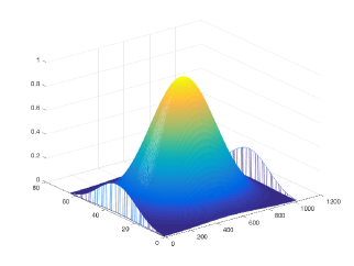
In the pre-permutation windowing and the flat-windowing stages, the window for each dimension is designed separately. After that, the high dimension widow is generated by combining each 1-D window. For instance, in the 2-D case, assuming that and are the two windows in the and dimension, respectively, a 2D window can be computed as
| (9) |
Fig. 2 shows a compound 2-D window which is a combination of a 64-point and a 1024-point Dolph-Chebyshev window, both of which has attenuation for the side-lobes in frequency domain. A Dolph-Chebyshev window allows us to trade off frequency resolution and side-lobe attenuation easly. Other windows sharing the same flexibility includes Gaussian window, Kaiser-Bessel window, Blackman-Harris window, etc., see [16] for detail. We apply those windows on the data by point-wise multiplications.
III-C2 Permutation
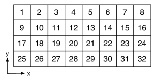
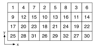
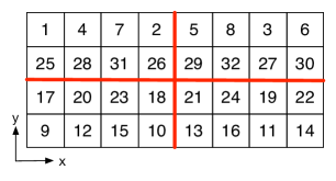
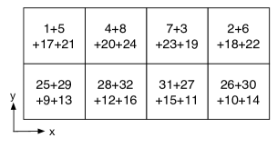
The permutation parameters are generated for each dimension in a random way according to (2). Then, we carry the permutation on each dimension sequentially. An example for the 2-D case is illustrated in Fig. 3.
III-C3 Aliasing
The aliasing stage compresses the high dimensional data into much smaller size. In 2-D, as shown in Fig. 3, a periodic extension of the data matrix is created with period in the dimension and in the dimension, with and , and the basic period, i.e., is extracted.
III-C4 First-stage-detection and reverse-mapping
We carry first stage detection after taking the square of magnitude of N-D FFT on the aliased data. Each data point is then compared with a pre-determined threshold, and for those passing the thresholds, their indices are reversed map to the original space. The combination of the reverse mapped indices from each dimension provides the tentative locations of the original frequency components.
III-C5 Accumulation and second-stage-detection
The accumulation stage collects the tentative frequency locations found in the reverse mapping for each iteration, and the number of occurrences for each location is calculated after running over iterations. The second stage detection finds indices in each dimension for those whose number of occurrence pass the threshold of this stage.
Based on the above discussion, we summarize the RSFT in Algorithm 1. Comparing to the original SFT, we add pre-permutation windowing process on the input data and incorporate NP detection in both stages of detection.
Depending on the application, the iterations can be applied on the same input data with different permutations. Alternatively, each iteration could process different segments (see the signal model in (10)) of input data as indicated in Algorithm 1, and it can effectively reduce the variance of the estimation via RSFT, provided that the signal is stationary.
The Estimation procedure in the RSFT is similar to the original Estimation procedure, except that the recovered Fourier coefficients should be divided by the spectrum of the pre-permutation window, so that the distortion due to pre-permutation windowing is compensated. Moreover, using Location is sufficient for our radar application, for it can provide the location of significant frequencies, which is directly related to the parameters to be estimated. We also set in each permutation, since the random phase rotation does not affect the performance of a detector after taking magnitude of the signal in the intermediate stage.
Input: complex signal in any fixed dimension
Output: , sparse frequency locations of input signal
IV Optimal Thresholds Design in the RSFT
The main challenge in implementing the RSFT is to decide the thresholds in the two stages of NP detection. The applying of NP detection in the RSFT is not a straitforward extension on the SFT, in that the two stages are inter-connected, thus need to be jointly studied. In the following, we will show that the two asymptotically optimal thresholds are jointly founded with an optimization process. The analysis is carried in 1-D, while the generalization to high dimension is straitforward.
IV-A Signal Model and Problem Formulation
We model the signal in continuous time domain as a superposition of sinusoids as well as additive white noise. We then sample the signal uniformly both in I and Q channels with a sampling frequency above the Nyqvist rate. Assume the total sampling time is divided into consecutive equal length segments, each of which contains samples, and (i.e., the signal is sparse in frequency domain). Then for each time segment, i.e., , we have
| (10) |
where denotes for the complex sinusoid, with as its frequency, i.e.,
| (11) |
We further assume that is unknown deterministic quantity and is constant during the whole process, while the complex amplitude of the sinusoid, i.e., takes random value for each segment. More specifically, we model as a circularly symmetric Gaussian process with the distribution . Likewise, the noise is distributed as , where is -dimensional zero vector, and is unit matrix. We also assume each sinusoid and the noise are uncorrelated. In addition, the neighboring sinusoids are resolvable in the frequency domain, i.e., the frequency spacing of neighboring sinusoids is greater than , where is the 6.0-dB bandwidth[16] of a window that applies on . Note the signal model in (10) is also commonly used in array signal processing literature for Uniform Linear Array (ULA) settings (See e.g., [17]), in which the time samples in each segment is replaced by spatial samples from array elements, and a sample segment is referred as a time snapshot.
We want to detect and estimate each from the input signal. From a non-parametric and data-independent perspective, this is a classic spectral analysis and detection problem that can be solved by any FFT-based spectrum estimation method, for example, the Bartlett method followed by a NP detection procedure (see Appendix A). In that case, the FFT computes the signal spectrum on frequency bins, and the detection is carried on each bin to determine whether there exists a significant frequency. In what follows, we define the detection and estimation problem related to the design of the RSFT.
Let be the SNR of the sinusoid. Let us define the worst case SNR, i.e., , as
| (12) |
Let denote for the probability of detection for the sinusoid with , and the corresponding probability of false alarm on each frequency bin.
Problem 1.
For the signal defined in (10), find the optimal thresholds of the first and the second stage of detection in an asymptotic sense, such that they minimize for given . Also, characterize the tradeoff between computational complexity and as a function of various parameters.
In the following, we investigate the two stages of detection separately, then summarize the solution into an optimization problem.
IV-B First Stage Detection
The first stage detection is performed on each data segment. After pre-permutation windowing, permutation and flat-windowing, the input signal can be expressed as
| (13) |
where is the permutation parameter for the segment, which has an uniform random distribution; is the permutation matrix, which functions as (2) with ; , , where and are pre-permutation window and flat-window, respectively.
Regarding the design of the flat-window, we take its frequency domain main-lobe to have width , and choose its length in time domain as . As indicated in [2], it is possible to use less data in flat-windowing by choosing the length of less than , i.e., dropping some samples in each segment after the permutation. However, a reduced length window in the time domain would result in longer transition regions in the frequency domain and as a result the detection performance of the system would degrade, since a larger transition region would allow more noise to enter the estimation process.
The time domain aliasing can be described as
| (14) |
where ; is the sub-matrix of , which is comprised of the to the rows of . And .
The FFT operation on the aliased data can be expressed as
| (15) |
where is the DFT matrix. For the entry of , we have
| (16) |
where is the column of , i.e., , and .
Substituting (10) into (16), and taking the sinusoid, which we assume is the weakest sinusoid with its SNR equals to , out of the summation
| (17) |
Since is a linear combination of , it holds that
| (18) |
where
| (19) |
and
| (20) |
It is easy to see that is summation of weighted variance from each signal and noise component.
We now investigate the bin, where is mapped to, and we have the following claim.
Claim 1.
For a complex sinusoid signal, i.e., , after pre-permutation windowing, permutation with , flat windowing, aliasing and FFT, the highest amplitude of signal spectrum appears in at location
| (21) |
where .
Proof.
If we were applying DFT to , the highest amplitude of the spectrum would appear on the grid point closest to , i.e. . The pre-permutation windowing will not change the position of the highest peak, provided the window is symmetric. Then after permutation, the peak location dilates by modularly, and becomes . Finally, after flat-windowing and aliasing, the signal is ideally downsampled in the frequency domain, and the data length changes from to . Then the -point DFT exhibits the highest peak on grid point as desired. A visualization of this process is shown in Fig. 4. ∎
On assuming that only maps to bin , and that the side-lobes (leakage) are far below the noise level (owning to the two stages of windowing, which attenuate the leakage down to a desired level), the effect of leakage from other sinusoids can be ignored. Then we can approximate the variance of as
| (22) |
In case that multiple frequencies are mapped to the same bin (collision), (22) gives a underestimate of the variance. The probability of a collision occurring reduces as .
The bin , for which no significant frequency is mapped to, contains only noise, and the corresponding variance for is
| (23) |
Hence, the hypothesis test for the first-stage-detection on is formulated as
-
•
: no significant frequency is mapped to it.
-
•
: at least one significant frequency is mapped to it, with worst case SNR equals to .
The log likelihood ratio test (LLRT) is
| (24) |
where and are the probability density function (PDF) of under and respectively, and is a threshold.
Substituting the PDF of under both hypothesis into (24), and after some manipulations we get
| (25) |
Hence, is a sufficient statistics for first stage detection. Since has circularly symmetric Gaussian distribution, is exponentially distributed with cumulative distribution function (CDF)
| (26) |
where equals to under and under .
Based on (26), in the first stage of detection, the false alarm rate on each of bins and the probability of detection of the weakest sinusoid can be derived to be equal to
| (27) |
where is the detection threshold. Both and depend on the permutation . Taking expectation with respect to , we have
| (28) |
where , , , and .
IV-C Second Stage Detection
Let denote the output of the first-stage-detection for the segment, with permutation factor . Each entry in is a Bernoulli random variable, i.e., for ,
| (29) |
Note that under , we assume that corresponds to the weakest sinusoid. For the other co-existing sinusoids, since their SNR may be grater than , their probability of detection may also be grater than (see Claim 3).
The reverse-mapping stage hashes the -dimensional back to the -dimensional . According to Definition 4, it holds that
| (30) |
After accumulation of iterations, each entry in the accumulated output is summation of Bernoulli variables with different success rate. Define as the accumulated output, then for its entry, we have
| (31) |
Note that in (31), each term inside the sum corresponds to a different segment, i.e., is from the segment. Since is drawn randomly for each segment, may take different values, and relates to via a reverse-mapping. Fig. 5 gives a graphical illustration of the mapping and reverse-mapping.
Now, the hypothesis test for the second-stage-detection on is formulated as
-
•
: no significant frequency exists.
-
•
: there exists a significant frequency, whose SNR is at least .
In the following, we investigate the statistics of under both hypothesis in an asymptotic senses. Before that however, we will take a closer look at the mapping and the reverse mapping by providing the following properties.
Property 3.
(Reversibility): Let . and satisfy Eq. (1). If , then it holds that
| (32) |
Property 4.
(Distinctiveness): Let . If and satisfies Eq. (1), then it holds that
| (33) |
The proofs of these properties are provided in Appendix B. The two properties simply reveal the following facts: a mapped location can be recovered by reverse mapping (with ambiguities). Also, when applying reverse mapping to two distinct locations with the same permutation parameter, the resulting locations are also distinct.
Under , assuming that corresponds to the sinusoid, i.e., the weakest sinusoid, then each term inside the sum of (31) has distribution . Then we present the following claim.
Claim 2.
Under , and as ,
| (34) |
where , .
Proof.
Since , for , the Lyapunov Condition[18] holds, i.e.,
| (35) |
Therefore, conforms to the Normal distribution as indicated in (34). It also holds that
| (36) |
from which we get that , with the equality holding when .
∎
The distribution of under is more complicated, and we have following claim.
Claim 3.
Under , and as ,
| (37) |
where
| (38) |
and , where is the 6.0-dB bandwidth of the pre-permutation window . is a calibration factor of the probability of detection for the other co-existing sinusoids.
Proof.
Under , each term in (31) may be distributed differently. To illustrate this, we consider a location in the frequency domain of the input signal, which does not contain a significant frequency, as shown in Fig. 5. Let be the mapping. There would be two cases for : 1) does not contain a significant frequency; or 2) contains at least one significant frequency, with its SNR at least . In the former case, , i.e., is under . For the latter case, , i.e., is under . Due to the permutation being uniformly random, on the average, the number of under is , and the number of under is . The parameter reflects the fact that sparsity is affected by the pre-permutation windowing. Since we assume that has the minimum SNR, i.e., , other sinusoids with higher SNR will have larger . Hence we multiply with to calibrate the successful rate of under . If all the sinusoids’s SNR were equal to , then ; on the other hand, if the co-existing sinusoids’ SNR were sufficient high so that their approaches to , then . Finally, the results follows immediately by applying Lyapunov CLT. ∎
Remark 1.
From Claim 2 and 3, we notice that for the second stage detection, the LLRT is obtained based on two Normal distributions. The test statistic under is “stable”, for it only depends on . However, under , the distribution depends on the number of co-existing sinusoids, as well as on each sinusoid’s SNR. The larger and higher SNR will “push” the distribution under closer to the distribution under , hence degrades the detection performance. In order to compensate for this, a larger is required.
A natural extension of Remark 1 is Remark 2, which gives the condition under which the RSFT will reach its limit.
Remark 2.
Assuming that , the RSFT will fail if no matter how large the is.
Proof.
Assuming and substituting into yields , which means that the distributions under both hypothes are the same, hence the two hypothesis cannot be discriminated. If , the assumption of will be violated as approaching . ∎
Based on the above discussion, the optimal threshold design in Problem 1 can be solved by the following optimization problem, i.e.,
| (39) |
where are the asymptotic PDF222We take the upper bounds of the variances in both distributions. It is shown in Section V-E that the actual variances is close to their upper bounds. of (which corresponds the weakest sinusoid) under and , respectively. Since both of them are Normal distributions, with fixed threshold, i.e., , we can solve for , and then compute the . By enumerating , the minimum worst case SNR, i.e., can be found, and the corresponding is the optimal threshold for the second stage of detection. The optimal threshold for the first stage of detection, i.e., , can thus be calculated via (28).
Remark 3.
In Claim 3, we set a parameter to calibrate the distribution of under . By setting as or , we can get respectively the lower and upper bound of for the variation of SNR of other co-existing sinusoids. If is the maximum budget of signal sparsity, the optimal thresholds found by solving (39) provides the optimal thresholds for the worst case. If the actual signal sparsity were less than , would be lower than the expected value, while would be unchanged according to Remark 1.
By averaging over the permutation, asymptotically, does not depend on the permutation. However, it still depends on , and we have the following claim to manifest their relationship.
Claim 4.
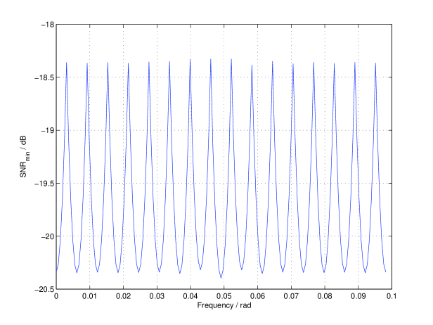
The dependence of on is due to the off-grid loss[16] from off-grid frequencies. attains its minimum when is on-grid, i.e. . When is in the middle of two grid points, i.e., , attains its maximum.
Proof.
Assume . Since the pre-permutation window is symmetric, if we applied DFT to the pre-permuted data, the amplitude of the spectrum would attain its maximum and minimum respectively when is on-grid or in the middle between two grid points. The subsequent permutation operation would not change the amplitude of the spectrum. Also, since the flat-window is used, the downsampling in the frequency domain, which is a result of aliasing, will not affect the amplitude either. The on-grid frequency generates highest amplitude, while the frequency in the middle of between grid points has the lowest amplitude. As a result, the two detection stages require the lowest SNR for on-grid frequencies, and the highest SNR for frequencies lying in the middle of between grid points. ∎
IV-D Tradeoff between Worst Case SNR and Complexity
IV-D1 Comparison to Bartlett Method
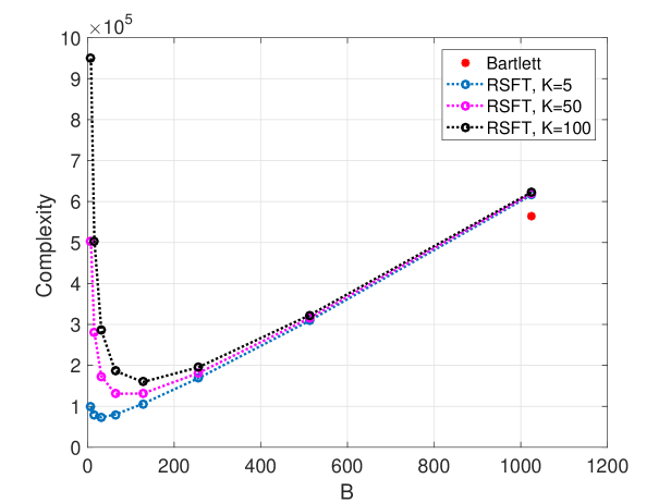
We compare the complexity of the RSFT with the FFT-based Bartlett method (see Appendix A) by counting the number of operations in both algorithms as shown in Table (I) and Table (II). The RSFT has complexity equal to
| (40) |
while the Bartlett method has complexity equal to . Fig. 6 compares the RSFT’s complexity to that of Bartlett’s for various and . One can see that the RSFT enabled savings are remarkable when is chosen properly. Specifically, from Fig. 6 one can see, the lowest complexity for equals to is achieved when equals to , respectively. Note that the core operation in RSFT is still FFT-based, but on a reduced dimension space. By leveraging the existing high performance FFT libraries such as FFTW [19], the implementation of the RSFT algorithm could be further improved.
Remark 4.
The complexity of RSFT is linearly depend on and , hence it is beneficial to choose a pre-permutation window with a small , provided the attenuation of the side-lobes is sufficient. We can also choose the optimal from (40) to minimize the computation. However, there are two additional constrains for , one is should be a power of 2, the other is , as stated in Remark 2.
| Procedure | Number of Operations |
|---|---|
| Windowing | |
| FFT | |
| Square | |
| Detection | |
| Complexity |
| Procedure | Number of Operations |
|---|---|
| Pre-Permutation Win | |
| Permutation | |
| Flat-Win | |
| Aliasing | |
| FFT | |
| Square | |
| First-Stage-Detection | |
| Reverse-Mapping | |
| Second-stage-Detection | |
| Complexity |
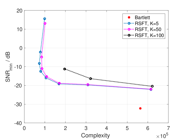
IV-D2 Worst Case SNR and Complexity Trade Off
The reduced complexity of RSFT is achieved at a the cost of an increased , which decreases the ability of detecting weak signals. The tradeoff between and complexity for various choices of parameters is shown in Fig. 7. The performance of the Bartlett method is also shown as a reference. From Fig. 7 we can see that plays a central role in trading off and complexity. A proper choice of can enhance the computational efficiency significantly with a reasonable increase of . Also, since the sparsity affects both and complexity, a less sparse signal will worsen both. The complexity of RSFT is larger than that of the Bartlett method by setting , due to the additional processing in the algorithm. Also, it cannot achieve the same as the Bartlett method does.
V Numerical Results
In this section, we verify our theoretical findings via simulations. We use the following common parameters for various settings, unless we state specifically. We take the following values: . We use a Dolph-Chebyshev window with attenuation as pre-permutation windowing. The flat-window is also based on this window, and we set its passband width as .
V-A Lower and Upper Bounds of for Fixed Sparsity
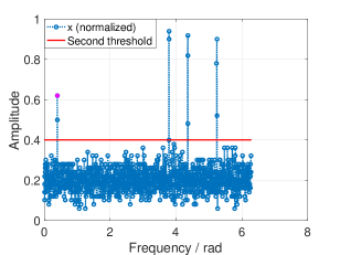
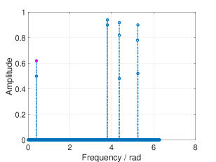
According to Remark 3, we can calculate the lower bound and the upper bound of and their corresponding thresholds for fixed sparsity. Fig. 8 and 9 shows the thresholding of RSFT with both bounds. We mark the amplitude of with a magenta dot in each figure.
V-B Unknown Signal Sparsity
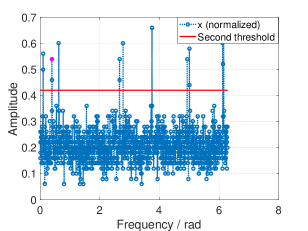
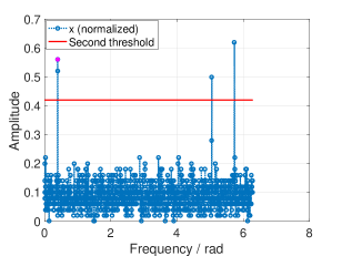
Since we do not assume that we know the exact sparsity of the signal, we will use a guess for . Fig. 10 shows the optimal design was toward , however, when the true sparsity is , the system yields the same but better , since the noise level is much lower than expected.
V-C Dependency on Frequency
V-D The Receiver Operating Characteristic (ROC) Curve
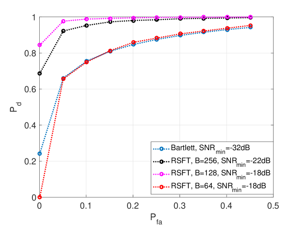
In this section, we use ROC curve to characterize the performance of RSFT with variance parameters. Fig. 12 shows the impact of the detection by adopting different values of . A smaller lowers the detection performance, and in order to compensate it, a higher is required. The ROC curve for the Bartlett method is calculated by (50) and is also shown in Fig. 12.
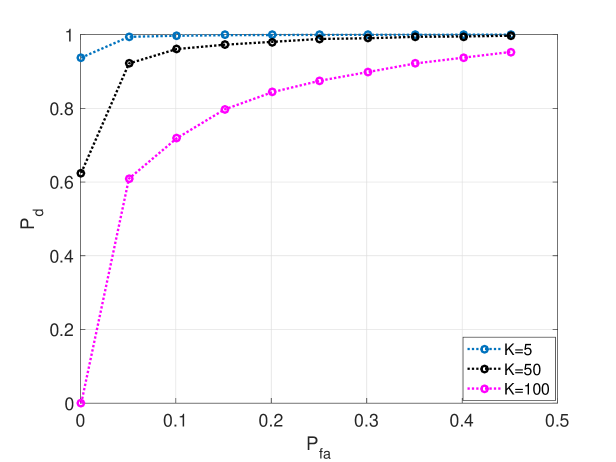
Fig. 13 illustrates the relationship between detection performance and sparsity of signal. It is shown that with other parameters fixed, the sparser the signal is, the better the performance of detection is.
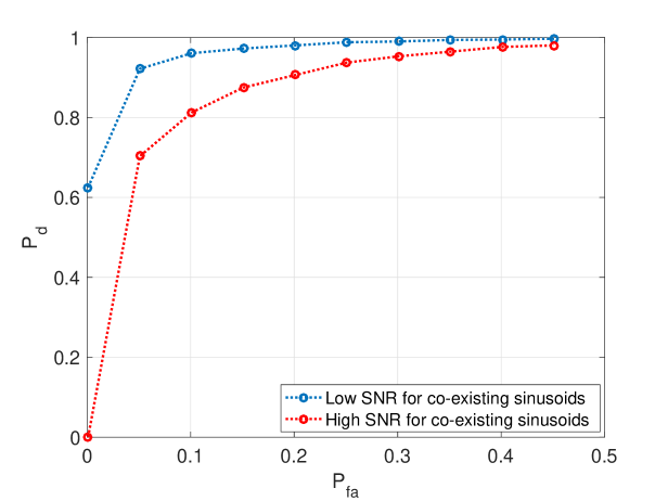
In Fig. 14, we can see the impact of the SNR from the co-existing sinusoids. The higher the SNR of the co-existing sinusoids is, the worse the detection performance is.
V-E The Variance and Its Upper Bound for
In solving (39), we take the upper bound of the variance for under both hypotheses. In this section, we show by simulation that the actual variance of is close to its upper bound. In what follows, we study ; the case for can be similarly studied.
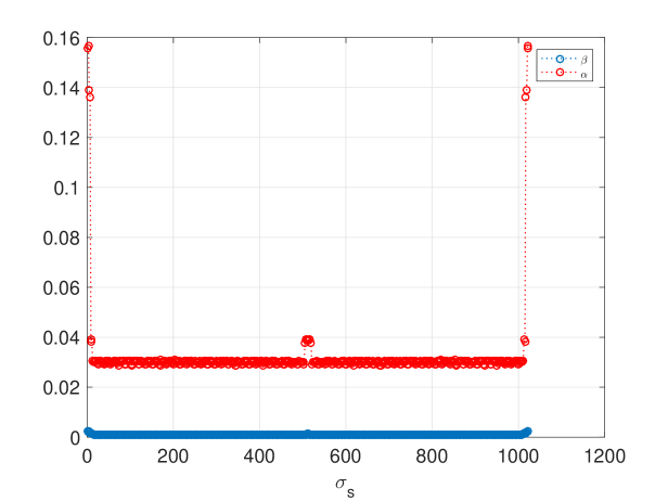
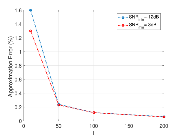
As shown in (36), the discrepancy of from its upper bound is due to the ’s dependence on , which is caused by and ’s dependence on (see (27)). For a power of 2, a valid can be any odd integer in [2]. Fig. 15 shows and as functions of . The symmetry of the plot is due to the symmetry of pre-permutation window and the flat-window, as well as the modulo property of the permutation. Another observation is that most of and have similar values. As a result, has similar value for different permutations, and this is the reason for being close to its upper bound. The Monte Carlo simulation in Fig. 16 shows that the approximation error, i.e., decreases as grows, and even for a small , such as , the error is as small as about .
VI RSFT for Ubiquitous Radar Signal Processing
The RSFT algorithm can greatly reduce the complexity of certain high dimensional problems. This can be signifiant in many applications, since lower complexity means faster reaction time and more economical hardware. However, in order to apply RSFT, the signal to be processed should meet the following requirements:
-
•
It should be sparse in some domain.
-
•
It should be sampled uniformly whether in temporal or spacial domain.
-
•
The SNR should be moderately high.
While many applications satisfy these requirements, in what follows, we discuss an example in Short Range Ubiquitous Radar[20] (SRUR) signal processing.
VI-A Short Range Ubiquitous Radar
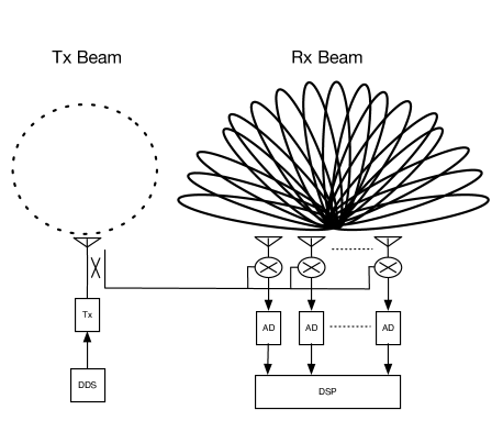
An ubiquitous radar or SIMO radar can see targets everywhere at anytime without steering its beams as a traditional phased array radar does. In SRUR, a broad transmitting beam patten is achieved by an omnidirectional transmitter and multiple narrow beams are formed simultaneously after receiving of the reflected signal. The beam pattens of an ubiquitous radar is shown in Fig. 17 with an Uniform Linear Array (ULA) configuration.
An SRUR with range coverage of several kilometers could be important both in military and civilian vehicular applications. For instance, in an active protection system [21], sensors on the protected vehicle have to detect and locate the warheads from a closely fired rocket-propelled grenade (RPG) within milliseconds. Among other sensors, SRUR’s simultaneous wide angle coverage, high precision of measurement and all-weather operation make it the ideal sensor for such situation.
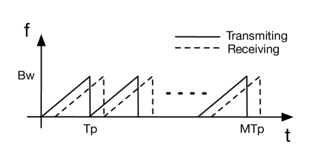
In order to achieve high range resolution and cover near range, SRUR utilizes a LFMCW waveform, as shown in Fig. 18. Mathematically, the transmitted waveform can be expressed as
| (41) |
where is the repetition interval (RI), denotes the RI, is amplitude of the signal, is the carrier frequency and is the chirp rate. Furthermore, without loss of generality, we assume that the initial phase of the signal is zero.
Upon reception, a de-chirp process is implemented by mixing the received signal with the transmitted signal, followed by a lowpass filter. The received signal is a delayed version of the transmitted one, hence by mixing the two signals, the range information of the targets is linearly encoded in the difference of the frequencies. Hence for the receiving channel, the de-chirped signal is expressed as
| (42) |
which is a superposition of sinusoids and additive noise . For the sinusoid, represents its amplitude, which can be modeled as a Gaussian random process. More specifically, the amplitude is assumed static within a burst, and independent between each of bursts. This assumption is consistent with the Swerling-I target model[22], which represents a slow fluctuation of the target RCS. are the frequency components respect to target’s range and velocity respectively, i.e.,
| (43) |
where are the target’s range, velocity and speed of wave propagation respectively.
The DOA of the target, i.e., is defined as the angle between the line of sight (from the array center to the target) and the array normal. Assuming that the element wise spacing is , under the narrowband signal assumption, will cause an increase of phase at the neighboring array element equal to . We omit the constant phase term in each sinusoids of (42), since they are irrelevant to the performance of the algorithm.
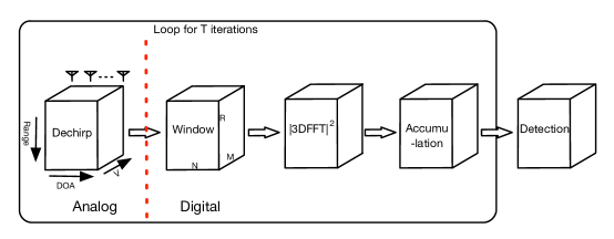
After AD conversion of each receiving channel, we can use the processing scheme shown in Fig. 19 to detect the targets as well as estimate their range, velocity and DOA. More specifically, grid-based versions of can be calculated by applying a 3-D FFT on the windowed data cube, then, after accumulation of iterations, the above described NP detection procedure can be performed.
VI-B RSFT-based SRUR Signal Processing
Although the number of samples of SRUR is reduced significantly with the analog de-chirp processing, the realtime processing with 3-D FFT is still challenging. The RSFT algorithm is suitable for reducing the computational complexity of SRUR, since, 1) the number of targets is usually much smaller than the number of spatial resolutions cells, which implies that the signal is sparse after proper translation; 2) with a ULA and digitization of each received element, the signal is uniformly sampled both in spatial and temporal domain; and 3) the short range coverage implies that moderate high SNR is easy to achieve.
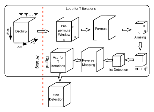
The RSFT-based SRUR processing architecture is shown in Fig. 20. Compared to the conventional processing, the 3-D FFT is replaced with a 3-D RSFT, in which the aliasing procedure converts the data cube dimensions from to . The 3-D FFT operated on the smaller data cube could save the computation time significantly.
VI-C Simulations
In this section, we verify the feasibility of RSFT-based SRUR processing and compare to the SFT-based processing via simulations. The main parameters of the system are listed in Table III. The design of the system can guarantee non-ambiguous measurements of the target’s range and velocity, assuming the maximum range and velocity are less than and , respectively.
| Parameter | Symbol | Value |
|---|---|---|
| Number of range bins | ||
| Number of receiving elements | ||
| Number of RI | ||
| Wave length | ||
| Wave propagation speed | ||
| Bandwidth | ||
| Repetition interval | ||
| Maxima range | ||
| Chirp rate | ||
| Sampling frequency (IQ) |
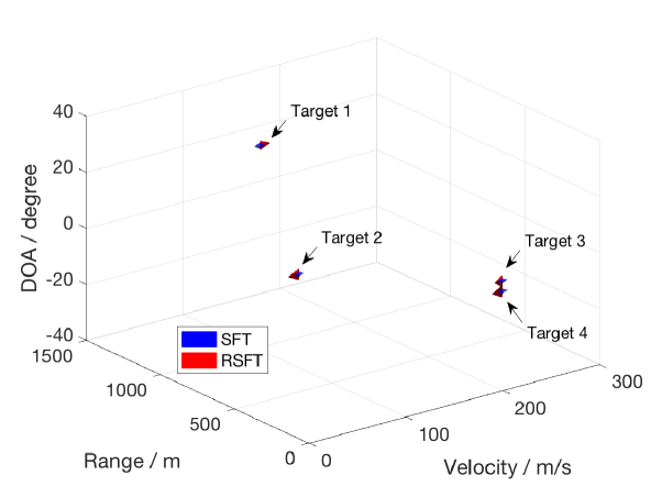
We generate signals from targets according to (42). The range, velocity and DOA of targets can be arbitrarily chosen within the unambiguous space, which implies that the corresponding frequency components do not necessarily lie on the grid. The targets’ parameters used in the simulation are listed in Table IV. For Targets and , we set the same parameters except that their DOA is apart, which is close to the theoretical angular resolution after windowing for the Bartlett beamforming. To compare the RSFT and the SFT for different scenarios, we adopt two sets of SNR for targets. Specifically, for the first set, we use the same SNR, i.e., for different targets. And for the second set, we assign different SNR for different targets, which is more close to a realistic scenario.
| Target | Range () | Velocity () | DOA () | SNR (dB) |
|---|---|---|---|---|
| 1 | ||||
| 2 | ||||
| 3 | ||||
| 4 |
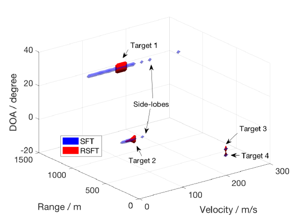
The SFT from [2] is -dimensional. In order to reconstruct targets in the 3-D space, we extend the SFT to high dimension with the techniques described in Section III-C. Another obstacle of applying SFT is that it needs to know the number of peaks to count in the detection stages. In our radar example, even the knowledge of exact number of targets is presented, it is still not clear how to determine the number of counting peaks due to existence of the large number of peaks from leakage. In the experiment, we gradually increase the number of counting peaks until all the targets are recovered. For the case of the same SNR setting, all the targets are recovered after around peaks are counted. While for the second SNR setting, we need to count nearly peaks to recover the weakest targets (Targets and ). Fig. 21 and 22 show the targets reconstruction results for the two settings, respectively. The former shows both SFT and RSFT methods can perfectly recover all the targets, whose SNR has the same value. From Targets and we can see that the SFT-based method achieves a better resolution than its RSFT counterpart, since the former does not require a pre-permutation window. For the second scenario, the SFT-based method shows the side-lobes of the stronger targets, while the RSFT-based method only recovers the (extended) main-lobes of all the targets.
The simulation shows that the RSFT-based approach is better than its SFT counterpart for a realistic scenario, within which the signal has a reasonable dynamic range. We also want to emphasis that in a real radar system, determine the number of counting peaks for the SFT-based method lacks a theoretical foundation, while the thresholding approach in the RSFT is consistent with the conventional FFT-based processing, both of which are based on the NP criterion.
VII Conclusion
In this paper, we have addressed practical problems of applying SFT in real-life applications, based on that, we have proposed a modified algorithm (RSFT). The optimal design of parameters in RSFT has been analyzed, and the relationship between system sensitivity and computational complexity has been investigated. Some interesting properties of the RSFT have also been revealed by our analysis, such as the performance of detection not only relies on the frequency under examination, but also depends on other co-existing significant frequencies, which is very different from the traditional FFT-based processing. The analysis has revealed that RSFT could provide engineers an extra freedom of design in trading off system’s ability of detecting weak signals and complexity. Finally, the context of the application of RSFT has been discussed, and a specific example for short range ubiquitous radar signal processing has been presented.
Appendix A Bartlett Method Analysis
Detecting each sinusoid and estimating the corresponding frequencies in (10) can be achieved by Bartlett spectrum analysis followed by an NP detection. A window is applied on each data segment to reduce the leakage of off-grid frequencies. In order to enhance the computational efficiency, the FFT is adopted (see Algorithm 2). In the -dimensional case, each step in Algorithm 2 is done in -dimension.
The analysis of the Bartlett method can be found in the literature [23], however, such analysis usually focuses on bias, variance and frequency resolution, while the detection performance has not been throughly studied in connection with an NP detector. In [24], the performance of detecting a single sinusoid is discussed and the theoretical analysis is provided for on-grid frequency. However, most typically, the signal contains multiple significant frequencies, which are off-grid. In what follows, we analyze the asymptotic performance of Algorithm 2 based on the signal model of (10), which is a multiple-frequencies case and does not restrict the frequency being on-grid. Moreover, as compared to the signal model in [24], which assumes that the sinusoid has a deterministic amplitude, we model the complex amplitude of each sinusoid as a circularly symmetric Gaussian random variable. This modeling reflects the stochastic nature of each sinusoid, and is consistent with the Swerling-I target model in radar signal cases, since the square of a circularly symmetric Gaussian random variable has an exponential distribution.
Input: complex signal in any fixed dimension
Output: , frequency domain representation of input signal
The analysis of Algorithm 2 follows a similar fashion with the analysis of the RSFT, and we thus use the same notation as in Section IV. Our goal is to derive the relationship between and , which is also related to the worst case signal SNR, i.e., .
After windowing and FFT, the signal becomes
| (44) |
where is the DFT matrix.
Since is a linear combination of , it is a circularly symmetry Gaussian scalar with distribution
| (46) |
The hypothesis test on each frequency bin is formulated as
-
•
: no significant frequency exists.
-
•
: there exists a significant frequency, with its SNR at least equals to .
We assume the side-lobes of the significant frequencies are far below the noise level due to windowing, then under and , respectively, we have the following approximation for
| (47) |
where and .
The LLRT yields the sufficient statistics
| (48) |
We study its asymptotic performance. Assume that is moderately large, after applying central limit theory, the test statistic distributes as Normal distributions in both hypothesis, i.e.,
| (49) |
Appendix B Proof of Properties of Mapping and Reverse Mapping
B-A Proof of Property 3
Proof.
According to Definition 3, the mapping can be split into two stages: 1) apply modular multiplication to , i.e., ; and, 2) convert into with .
Similarly, according to Definition 4, the reverse-mapping also can be split into two stages: 1) dilate into ; and, 2) apply inverse modular multiplication on , i.e., .
The first stage of reverse-mapping is the inverse operation of the second stage of mapping, and as a result, . Hence as desired. ∎
B-B Proof of Property 4
Proof.
We use the two stages of the reverse-mapping in the proof of Property 3. The first stage of the reverse-mapping for and yields and , respectively. It is not difficult to verify that , provided that .
In what follows, we will prove that the second stage of the reverse-mapping also gives distinct results. Assume that there exists , such that . Modularly multiply both sides with yields that , which is contradictory with . Hence both stages of the reverse-mapping guarantee the results are distinct for . ∎
Acknowledgment
The authors would like to thank Dr. Predrag Spasojevic and Dr. Anand Sarwate from Rutgers university for initial support of this work. The work of SW was jointly supported by China Scholarship Council and Shanghai Institute of Spaceflight Electronics Technology. The work of VMP was partially supported by an ARO grant W911NF-16-1-0126.
References
- [1] H. Hassanieh, P. Indyk, D. Katabi, and E. Price, “Nearly optimal sparse fourier transform,” in Proceedings of the forty-fourth annual ACM symposium on Theory of computing, pp. 563–578, ACM, 2012.
- [2] H. Hassanieh, P. Indyk, D. Katabi, and E. Price, “Simple and practical algorithm for sparse fourier transform,” in Proceedings of the Twenty-third Annual ACM-SIAM Symposium on Discrete Algorithms, SODA ’12, pp. 1183–1194, SIAM, 2012.
- [3] F. Ong, S. Pawar, and K. Ramchandran, “Fast and efficient sparse 2d discrete fourier transform using sparse-graph codes,” arXiv preprint arXiv:1509.05849, 2015.
- [4] A. C. Gilbert, P. Indyk, M. Iwen, and L. Schmidt, “Recent developments in the sparse fourier transform: A compressed fourier transform for big data,” Signal Processing Magazine, IEEE, vol. 31, no. 5, pp. 91–100, 2014.
- [5] B. Ghazi, H. Hassanieh, P. Indyk, D. Katabi, E. Price, and L. Shi, “Sample-optimal average-case sparse fourier transform in two dimensions,” in Communication, Control, and Computing (Allerton), 2013 51st Annual Allerton Conference on, pp. 1258–1265, IEEE, 2013.
- [6] P. Indyk and M. Kapralov, “Sample-optimal fourier sampling in any constant dimension,” in Foundations of Computer Science (FOCS), 2014 IEEE 55th Annual Symposium on, pp. 514–523, IEEE, 2014.
- [7] H. Hassanieh, F. Adib, D. Katabi, and P. Indyk, “Faster gps via the sparse fourier transform,” in Proceedings of the 18th annual international conference on Mobile computing and networking, pp. 353–364, ACM, 2012.
- [8] H. Hassanieh, L. Shi, O. Abari, E. Hamed, and D. Katabi, “Ghz-wide sensing and decoding using the sparse fourier transform,” in INFOCOM, 2014 Proceedings IEEE, pp. 2256–2264, IEEE, 2014.
- [9] L. Shi, H. Hassanieh, A. Davis, D. Katabi, and F. Durand, “Light field reconstruction using sparsity in the continuous fourier domain,” ACM Transactions on Graphics (TOG), vol. 34, no. 1, p. 12, 2014.
- [10] A. Rauh and G. R. Arce, “Sparse 2d fast fourier transform,” Proceedings of the 10th International Conference on Sampling Theory and Applications, 2013.
- [11] P. Boufounos, V. Cevher, A. C. Gilbert, Y. Li, and M. J. Strauss, “What’s the frequency, kenneth?: Sublinear fourier sampling off the grid,” in Approximation, Randomization, and Combinatorial Optimization. Algorithms and Techniques, pp. 61–72, Springer, 2012.
- [12] E. J. Candè and M. B. Wakin, “An introduction to compressive sampling,” Signal Processing Magazine, IEEE, vol. 25, no. 2, pp. 21–30, 2008.
- [13] C.-Y. Chen and P. Vaidyanathan, “Compressed sensing in mimo radar,” in Signals, Systems and Computers, 2008 42nd Asilomar Conference on, pp. 41–44, IEEE, 2008.
- [14] Y. Yu, A. P. Petropulu, and H. V. Poor, “Mimo radar using compressive sampling,” Selected Topics in Signal Processing, IEEE Journal of, vol. 4, no. 1, pp. 146–163, 2010.
-
[15]
S. Wang, V. M. Patel, and A. Petropulu, “RSFT: a realistic high dimensional
sparse fourier transform and its application in radar signal processing,” in
Milcom 2016 Track 1 - Waveforms and Signal Processing., (Baltimore,
USA), Avaliable at:
http://www.rci.rutgers.edu/ vmp93/Conference_pub/
MILCOM2016_SFT.pdf, Nov. 2016. - [16] F. J. Harris, “On the use of windows for harmonic analysis with the discrete fourier transform,” Proceedings of the IEEE, vol. 66, no. 1, pp. 51–83, 1978.
- [17] H. L. Van Trees, Optimum array processing: part IV of detection, estimation, and modulation, ch. 5, pp. 349–350. Wiley, New York, 2002.
- [18] R. B. Ash and C. Doleans-Dade, Probability and measure theory, p. 309. Academic Press, 2000.
- [19] M. Frigo and S. G. Johnson, “Fftw: An adaptive software architecture for the fft,” in Acoustics, Speech and Signal Processing, 1998. Proceedings of the 1998 IEEE International Conference on, vol. 3, pp. 1381–1384, IEEE, 1998.
- [20] M. Skolnik, “Systems aspects of digital beam forming ubiquitous radar,” tech. rep., DTIC Document, 2002.
- [21] D. A. Schade, T. C. Winant, J. Alforque, J. Faul, K. B. Groves, V. Horvatich, M. A. Middione, C. Tarantino, and J. R. Turner, “Fast acting active protection system,” Apr. 10 2007. US Patent 7,202,809.
- [22] M. I. Skolnik, “Radar handbook,” 1970.
- [23] P. Stoica and R. L. Moses, Spectral analysis of signals, pp. 49–50. Pearson/Prentice Hall Upper Saddle River, NJ, 2005.
- [24] H. So, Y. Chan, Q. Ma, and P. Ching, “Comparison of various periodograms for sinusoid detection and frequency estimation,” Aerospace and Electronic Systems, IEEE Transactions on, vol. 35, no. 3, pp. 945–952, 1999.