An efficient method for computing genus expansions and counting numbers in the Hermitian matrix model

Gabriel Álvarez galvarez@fis.ucm.es Luis Martínez Alonso luism@fis.ucm.es Elena Medina elena.medina@uca.es Departamento de Física Teórica II, Facultad de Ciencias Físicas, Universidad Complutense, 28040 Madrid, Spain Departamento de Matemáticas, Facultad de Ciencias, Universidad de Cádiz, 11510 Puerto Real, Spain

Abstract

We present a method to compute the genus expansion of the free energy of Hermitian matrix models from the large $N$ expansion of the recurrence coefficients of the associated family of orthogonal polynomials. The method is based on the Bleher-Its deformation of the model, on its associated integral representation of the free energy, and on a method for solving the string equation which uses the resolvent of the Lax operator of the underlying Toda hierarchy. As a byproduct we obtain an efficient algorithm to compute generating functions for the enumeration of labeled $k$ -maps which does not require the explicit expressions of the coefficients of the topological expansion. Finally we discuss the regularization of singular one-cut models within this approach.

keywords:

Hermitian matrix model , genus expansion , counting maps

MSC:

[2008] 14N10 , 82B41 , 15B52

^†^†journal: Nuclear Physics B

1 Introduction

In this paper we consider the ensemble of random Hermitian matrices

Z_{N}(\mathbf{g})=\int_{\mathbf{R}^{N}}\exp\left(-N\sum_{i=1}^{N}V(x_{i},\mathbf{g})\right)\prod_{i<j}(x_{i}-x_{j})^{2}\mathrm{d}x_{1}\cdots\mathrm{d}x_{N},

(1)

for a given polynomial potential

V(z,\mathbf{g})=\sum_{n=1}^{2p}g_{n}z^{n}

(2)

of degree $2p$ with real coefficients $\mathbf{g}=(g_{1},\ldots,g_{2p})$ such that $g_{2p}>0$ (we will not make explicit the dependence on $\mathbf{g}$ of the functions associated with the model (1) unless there is risk of ambiguity). For more than thirty years [1, 2, 3, 4, 5, 6] the asymptotic behavior of the free energy

F_{N}=-\frac{1}{N^{2}}\ln Z_{N}

(3)

as $N\rightarrow\infty$ and its relation to the counting of Feynman graphs have been subjects of intensive research. However, rigorous proofs of the existence of an asymptotic expansion of $F_{N}$ in powers of $N^{-2}$ were provided only rather more recently by Ercolani and McLaughlin [7] and by Bleher and Its [2]. These analyses prove the existence of a genus expansion of the form

F_{N}(\mathbf{g})-F_{N}^{\mathrm{G}}\sim\sum_{k\geq 0}F^{(k)}(\mathbf{g})N^{-2k},

(4)

where $F_{N}^{\mathrm{G}}$ stands for the Gaussian free energy,

F_{N}^{\mathrm{G}}=-\frac{1}{N^{2}}\ln\left(\frac{2\pi^{N/2}}{(2N)^{N^{2}/2}}\prod_{n=1}^{N}n!\right),

(5)

under the assumption that there is a path $\mathbf{g}(t)$ in the space of coupling parameters connecting $V(z,\mathbf{g})$ to the Gaussian potential $z^{2}$ in such a way that $V(z,\mathbf{g}(t))$ is a regular one-cut model for all $t$ . The functions $F^{(k)}(\mathbf{g})$ are important objects because the coefficients of their Taylor expansions at the Gaussian point $g_{k}^{\mathrm{G}}=\delta_{k,2}$ are generating functions for the enumeration of labeled $k$ -maps with vertices involving valences $1,\ldots,2p$ , where $2p$ is the number of nonvanishing coupling parameters $g_{n}$ . The general aim of the present work is the characterization of the structure of these functions $F^{(k)}(\mathbf{g})$ . (Incidentally, for multi-cut models it has been shown [8, 9] that in general the free energy exhibits an oscillatory behavior as a function of $N$ , and consequently topological expansions cannot exist.)

The large $N$ asymptotics of the matrix model (1) is intimately connected with the asymptotics of the recurrence coefficients $r_{n,N}$ and $s_{n,N}$ in the three-term recursion relation

xP_{n,N}(x)=P_{n+1,N}(x)+s_{n,N}P_{n,N}(x)+r_{n,N}P_{n-1,N}(x),

(6)

for the orthogonal polynomials $P_{n,N}(x)=x^{n}+a_{n-1}x^{n-1}+\cdots$ with respect to the exponential weight

\int_{-\infty}^{\infty}P_{k,N}(x)P_{l,N}(x)e^{-NV(x)}\mathrm{d}x=\delta_{k,l}h_{k,N}.

(7)

In particular [10, 11], in the limit

n\rightarrow\infty,\quad N\rightarrow\infty,\quad\frac{n}{N}\rightarrow T,

(8)

the density of zeros of $P_{n,N}(x)$ reduces to the eigenvalue density of the matrix model $Z_{N}(\mathbf{g}/T)$ , and if $Z_{N}(\mathbf{g}/T)$ is a regular one-cut model then [3, 12] the recurrence coefficients $r_{n,N}$ and $s_{n,N}$ can be expanded in powers of $N^{-2}$ [2].

The methods that exploit this relation with orthogonal polynomials to calculate the asymptotics of the free energy essentially consist of three steps:

1.

Determine the free energy in terms of the recurrence coefficients.
2.

Obtain the asymptotic expansion of the recurrence coefficients.
3.

Use 1 and 2 to obtain the asymptotic expansion of the free energy.

There are alternative methods based on solving the Ward identities for the partition function (loop identities) [13] (cf. also [14]) or on formulating the matrix model as a conformal field theory [15]. However, the structure of the expressions for the $F^{(k)}(\mathbf{g})$ that these methods provide is less suitable than ours to compute generating functions for the enumeration of labeled $k$ -maps.

In this paper we present an efficient method to calculate the topological expansion of the free energy and to characterize its coefficients. For simplicity we restrict our analysis to Hermitian models associated to even potentials $V(\lambda)$ , where $\lambda=z^{2}$ . We now preview how our approach performs the three steps and point out the differences with respect to other schemes.

The classical method of Bessis, Itzykson and Zuber [6, 16, 17, 18, 19, 20, 21] is based on the following identity (step 1):

F_{N}=-\frac{1}{N^{2}}\ln(N!)-\frac{1}{N}\left(\ln h_{0,N}+\sum_{n=1}^{N-1}\left(1-\frac{n}{N}\right)\ln r_{n,N}\right),

(9)

wherein the expansion of $r_{n,N}$ is substituted (step 2), and the asymptotic behavior of $F_{N}$ is obtained by means of the Euler-Maclaurin summation formula (step 3). However, some objections to this approach were raised by Ercolani and McLaughlin (cf. subsection 1.5 in [7]) due to the use of the asymptotic series of $r_{n,N}$ as a uniform expansion valid even for $n=1$ as $N\rightarrow\infty$ . This objection triggered the interest in alternative strategies for step 1 [2, 7, 22]. For example, Ercolani, McLaughlin and Pierce [22] derived a hierarchy of second order differential equations to determine the coefficients of the expansion (4) from those of the the asymptotic expansion of $r_{n,N}$ . In our work we use instead the Bleher-Its integral representation [2]

F_{N}(\mathbf{g})=F_{N}^{\mathrm{G}}+\int_{1}^{\infty}\frac{1-t}{t^{2}}\left[r_{N,N}({\mathbf{g}(t)})\left(r_{N-1,N}({\mathbf{g}(t)})+r_{N+1,N}({\mathbf{g}(t)})\right)-\frac{1}{2}\right]\mathrm{d}t.

(10)

where $\mathbf{g}(t)$ denotes the Bleher-Its deformation [2]

V(\lambda,\mathbf{g}(t))=(1-1/t)\lambda+V(\lambda/t,\mathbf{g}),\quad 1\leq t<\infty,

(11)

or explicitly in terms of the coupling parameters,

g_{2}(t)=1-\frac{1}{t}+\frac{g_{2}}{t},\qquad g_{2k}(t)=\frac{g_{2k}}{t^{k}},\quad k\geq 2.

(12)

For step 2 the standard methods [2, 5] use recursive equations for the coefficients $r_{n,N}$ (string equations) to determine expansions of the form

r_{n,N}(\mathbf{g})\sim\sum_{k\geq 0}r_{k}(T,\mathbf{g})\epsilon^{2k},\quad\epsilon=\frac{1}{N}.

(13)

Bessis, Itzykson and Zuber [17, 23] formulated the string equation in terms of summations of paths over a certain staircase. Some years later Shirokura [19, 20] developed a general method to perform these summations and characterize the coefficients of the expansion (13) in terms of the single function

W(r_{0},\mathbf{g})=\sum_{n=1}^{p}{2n\choose n}ng_{2n}r_{0}^{n}.

(14)

To solve the string equation, in this paper we introduce a generating function $U_{n,N}(\lambda)$ associated to the resolvent of the finite-difference Lax operator $L$ of the underlying Toda hierarchy [24]

LP_{n,N}=P_{n+1,N}+r_{n,N}P_{n-1,N},

(15)

and determine the coefficients of (13) from the function (14) as rational functions of the leading coefficient $r_{0}$ . This approach is simpler that Shirokura’s method, is particularly suitable for symbolic computation, can be applied to a generic potential, and permits an easy characterization of the asymptotics of the Bleher-Its deformation $r_{n,N}(\mathbf{g}(t))$ of the recurrence coefficient.

Finally, regarding step 3, the Bleher-Its representation (10) allows us to express the coefficients of the topological expansion as

F^{(k)}(\mathbf{g})=\int_{0}^{r_{0}}R_{k}(\xi,\mathbf{g})\mathrm{d}\xi,\quad k\geq 1,

(16)

where the integrands $R_{k}(\xi,\mathbf{g})$ are rational functions of $\xi$ which can be computed explicitly in terms of the function (14).

The layout of this paper is as follows. In section 2 we briefly review the basic facts about matrix models which are required to discuss the Bleher-Its deformation and the conditions that ensure the existence of the expansion (4). Then we apply our results to the quartic model and to the sixtic model of Brezin, Marinari and Parisi [25]. Section 3 is devoted to the asymptotic expansion (13) of the recurrence coefficient for general models $V(\lambda,\mathbf{g})$ and their respective Bleher-Its deformations $V(\lambda,\mathbf{g}(t))$ . In particular, we rederive in a much shorter way the expressions for the coefficients $r_{1}(T,\mathbf{g})$ and $r_{2}(T,\mathbf{g})$ found by Shirokura [19, 20]. Section 4 deals with the asymptotics of the free energy. From the Bleher-Its representation (10) and the expansion of the recurrence coefficients we obtain the integral expression (16). We evaluate explicitly the integrals for the $F^{(k)}$ up to genus 3 in the general case and find, except for a coefficient in the expression of $F^{(3)}$ , the same results found by Shirokura [19, 20]. We also check that the expressions of these coefficients for general two-valence models reduce to those obtained using the Ercolani-McLaughlin-Pierce method [22]. In the brief section 5 we discuss how to apply our method to compute counting maps functions and present explicit calculations for two and three valence models. In section 6 we formulate a “triple scaling” method to regularize the free energy expansion of a class of singular models (the singular one-cut case) and show how the Painlevé I hierarchy emerges in our approach. The paper ends with a brief summary.

2 The Bleher-Its deformation

To calculate the asymptotic behavior of $F_{N}(\mathbf{g})$ as $N\to\infty$ using the Bleher-Its formula (10) we need the asymptotics of the deformed recurrence coefficients $r_{n,N}({\mathbf{g}(t)})$ where $\mathbf{g}(t)$ is the Bleher-Its deformation of $\mathbf{g}$ . In this section we study the action of this deformation on the space of coupling parameters. As relevant examples we analyze the Bleher-Its deformation for models associated to quartic potentials and to the sixtic potentials of Brezin, Marinari and Parisi [25].

The continuum limit of $r_{n,N}(\mathbf{g}(t))$ depends on the number $q$ of cuts of the model $V(\lambda,\mathbf{g}(t))/T$ . In appendix A we summarize the method to determine the number of cuts of a generic hermitian model. The endpoints of a $q$ -cut eigenvalue support $J=\cup_{j=1}^{q}(\alpha_{j},\beta_{j})$ are the solutions of the system of $2q$ equations (181)–(183) but, in general, several such systems of equations corresponding to different values of $q$ may have admissible solutions for one and the same model. Among these candidate solutions, the correct value of $q$ is uniquely determined by the additional set of inequalities (184)–(186) on the polynomial $h(z)$ defined by

\frac{V_{z}(z)}{w_{1}(z)}=h(z)+\mathcal{O}(z^{-1})\quad\mbox{as }z\rightarrow\infty,

(17)

where $w_{1}(z)$ is the branch of the function

w(z)=\sqrt{\prod_{i=1}^{q}(z-\alpha_{i})(z-\beta_{i})}

(18)

with asymptotic behavior $w_{1}(z)\sim z^{q}$ as $z\rightarrow\infty$ . In turn, the polynomial $h(z)$ is related to the eigenvalue density $\rho(x)$ by

\rho(x)=\frac{h(x)}{2\pi\mathrm{i}}w_{1,+}(x)\quad\mbox{for }x\in J,

(19)

where $w_{1,+}(x)$ denotes the boundary value of $w_{1}(z)$ on $J$ from above.

We restrict our considerations to even potentials of the form

V(\lambda,\mathbf{g})=\sum_{j=1}^{p}g_{2j}\lambda^{j},\quad\lambda=z^{2},\quad g_{2p}>0,

(20)

where the coupling constants $\mathbf{g}=(g_{2},g_{4},\ldots,g_{2p})$ run on a certain region $G$ of $\mathbf{R}^{p}$ . The phase diagram of the corresponding family of matrix models is introduced through the decomposition

G=\bigcup_{q=1}^{p}\overline{G}_{q},

(21)

where $\mathbf{g}\in G_{q}$ if and only if $\mathbf{g}$ determines a $q$ -cut regular model (cf. appendix A). We will refer to $G_{q}$ as the $q$ -cut phase of the family (20) of Hermitian models. For even potentials the eigenvalue support $J$ is symmetric with respect to the origin, and in the one-cut case the endpoints of $J=(-\alpha,\alpha)$ are determined by the single equation (183), which in terms of $V$ reduces to

\oint_{\gamma}\frac{\mathrm{d}\lambda}{2\pi\mathrm{i}}V_{\lambda}(\lambda)\sqrt{\frac{\lambda}{\lambda-\alpha^{2}}}=1.

(22)

Regarding the behavior of a particular model $\mathbf{g}\in G$ with respect to its Bleher-Its deformation, we will consider two cases in our analysis: the regular one-cut case, in which ${\mathbf{g}(t)}\in G_{1}$ for all $t\geq 1$ , and the singular one-cut case in which ${\mathbf{g}(t)}\in G_{1}$ for $t>1$ but $\mathbf{g}=\mathbf{g}(1)$ determines a singular model (cf. appendix A).

2.1 The quartic model

The quartic model

V(\lambda,\mathbf{g})=g_{2}\lambda+g_{4}\lambda^{2}

(23)

in the region

G=\{\mathbf{g}=(g_{2},g_{4})\in\mathbf{R}^{2}:g_{4}>0\},

(24)

only exhibits $q=1$ and $q=2$ phases [26]. The $q=1$ phase $G_{1}$ can be written as the union

G_{1}=G_{1}^{(1)}\cup G_{1}^{(2)},

(25)

where

	$\displaystyle G_{1}^{(1)}$	$\displaystyle=$	$\displaystyle\{(g_{2},g_{4})\in\mathbf{R}^{2}:g_{2}\geq 0,g_{4}>0\},$		(26)
	$\displaystyle G_{1}^{(2)}$	$\displaystyle=$	$\displaystyle\{(g_{2},g_{4})\in\mathbf{R}^{2}:g_{2}<0,g_{4}>0,g_{2}>-2\sqrt{g_{4}}\},$		(27)

and the $q=2$ phase $G_{2}$ is given by

G_{2}=\{(g_{2},g_{4})\in\mathbf{R}^{2}:g_{4}>0,g_{2}<-2\sqrt{g_{4}}\}.

(28)

The phase diagram features the critical curve

g_{2}=-2\sqrt{g_{4}},

(29)

which demarcates the transition line between the two phases.

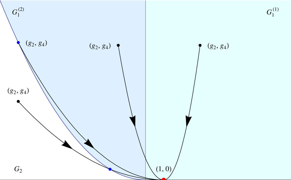
Consider now the Bleher-Its deformation (cf. figure 1)

{\mathbf{g}(t)}=(g_{2}(t),g_{4}(t))=\left(\frac{t-1+g_{2}}{t},\frac{g_{4}}{t^{2}}\right).

(30)

If $\mathbf{g}\in G_{1}^{(1)}$ then $g_{2}>0$ and $g_{2}(t)>0$ for all $t>1$ . Therefore ${\mathbf{g}(t)}\in G_{1}$ for all $t>1$ . If $\mathbf{g}\in G_{1}^{(2)}$ , then $g_{2}>-2\sqrt{g_{4}}$ and

g_{2}(t)=\frac{t-1+g_{2}}{t}>-2\frac{\sqrt{g_{4}}}{t}=-2\sqrt{g_{4}(t)}.

(31)

Hence if $\mathbf{g}\in G_{1}^{(2)}$ we also have that ${\mathbf{g}(t)}\in G_{1}$ for all $t>1$ . On the other hand, it is elementary to see that if $\mathbf{g}\in G_{2}$ or is on the critical curve (29) then ${\mathbf{g}(t_{0})}$ is on the critical curve for $t_{0}=1-g_{2}-2\sqrt{g_{4}}$ . Summing up,

1.

If $\mathbf{g}\in G_{1}$ then ${\mathbf{g}(t)}\in G_{1}$ for all $t\geq 1$ .
2.

If $\mathbf{g}\in G_{2}$ then ${\mathbf{g}(t)}$ crosses the critical curve at $t_{0}=1-g_{2}-2\sqrt{g_{4}}$ .
3.

If $\mathbf{g}$ is on the critical curve (29) then ${\mathbf{g}(t)}\in G_{1}$ for all $t>1$ .

Refer to caption — Figure 1: Deformation paths ${\mathbf{g}(t)}$ for the quartic potential. From left to right: a deformation of a two-cut regular model, a deformation in the singular one-cut case and two deformations in the regular one-cut case.

2.2 The Brezin-Marinari-Parisi model

In [25] Brezin, Marinari and Parisi considered the potentials $V(z)/T$ with

V(z)=90z^{2}-15z^{4}+z^{6}

(32)

to generate a non-perturbative ambiguity-free solution of a string model. The models $V(z)/T$ define a path in the space of coupling constants

G=\{\mathbf{g}=(g_{2},g_{4},g_{6})\in\mathbf{R}^{3}:g_{2}>0,g_{4}<0,g_{6}>0\}

(33)

of the family of even sixtic potentials

V(\lambda,\mathbf{g})=g_{2}\lambda+g_{4}\lambda^{2}+g_{6}\lambda^{3},\quad(\lambda=z^{2}).

(34)

We refer to appendix A for the proof of the following facts: (i) the inequality

\frac{5g_{2}g_{6}}{2g_{4}^{2}}>1

(35)

determines an open subset of the one-cut phase $G_{1}$ ; (ii) the boundary $\Gamma$ of this subset is the elliptic cone

5g_{2}g_{6}=2g_{4}^{2};

(36)

(iii) the sixtic model (34) is singular on the curve $\gamma$ given by

5g_{2}g_{6}=2g_{4}^{2},\quad 4g_{4}^{3}=-225g_{6}^{2};

(37)

and (iv) the model is in $G_{1}$ for $\mathbf{g}$ in $\Gamma-\gamma$ .

We apply these results to study the deformations of (32) from the initial point $\mathbf{g}=(90,-15,1)$ in $\Gamma$ . The homogeneity in $T$ of (36) implies that the curve $\mathbf{g}/T$ lies on $\Gamma$ for all $T>0$ , while from (37) it follows that $\mathbf{g}/T\in\gamma$ only at $T=60$ . Then $\mathbf{g}/T\in G_{1}$ for all $T\neq 60$ while $\mathbf{g}/60$ represents the multicritical string model of [25] with potential function

V_{c}(\lambda)=\frac{3}{2}\lambda-\frac{1}{4}\lambda^{2}+\frac{1}{60}\lambda^{3}.

(38)

Finally, if we apply first the Bleher-Its deformation to $V(\lambda,\mathbf{g}/T)$ the resulting coupling parameters are

g_{2}(T,t)=\left(1-\frac{1}{t}\right)+\frac{g_{2}}{tT},\qquad g_{4}(T,t)=\frac{g_{4}}{t^{2}T},\qquad g_{6}(T,t)=\frac{g_{6}}{t^{3}T}.

(39)

For the particular values $g_{2}=90$ , $g_{4}=-15$ , $g_{6}=1$ of (32) a direct computation shows that

\frac{5}{2}\frac{g_{2}(T,t)g_{6}(T,t)}{g_{4}(T,t)^{2}}=1+\frac{T(t-1)}{90},

(40)

and using (35) we find that $\mathbf{g}(T,t)\in G_{1}$ for all $T\neq 60$ and $t\geq 1$ .

3 Asymptotics of the recurrence coefficients

The main equation to determine the asymptotics of the recurrence coefficients is the discrete string equation [3]

V_{z}(L)_{n,n-1}=\frac{n}{N}.

(41)

Here $V_{z}$ stands for the derivative of the potential with respect to $z$

V_{z}(z)=\sum_{k=1}^{2p}2kg_{2k}z^{2k-1},

(42)

the subindex $(n,n-1)$ denotes the corresponding matrix element between the orthogonal polynomials

v_{n}(x)=P_{n,N}(x),\quad n\geq 0

(43)

defined in (7), and the operator $L$ acts on this family of polynomials as

Lv_{n}=v_{n+1}+r_{n,N}v_{n-1},\quad r_{0,N}=0.

(44)

The string equation (41) can be written in the form

\oint_{\gamma}\frac{\mathrm{d}\lambda}{2\pi\mathrm{i}}V_{\lambda}(\lambda)U_{n,N}(\lambda)=\frac{n}{N}\qquad(\lambda=z^{2}),

(45)

where $\gamma$ is a large positively oriented circle $|\lambda|=R$ , and $U_{n,N}$ is the generating function

U_{n,N}(\lambda)=1+2\sum_{k\geq 1}\left(L^{2k-1}\right)_{n,n-1}\lambda^{-k}.

(46)

Note that $L$ is the Lax operator of the Toda hierarchy [24] and that $U_{n,N}$ is related to the resolvent $\mathcal{R}(z)=(L-z)^{-1}$ of $L$ by

U_{n,N}(\lambda)=1-\mathcal{R}(z)_{n,n-1}-\mathcal{R}(-z)_{n,n-1}.

(47)

In appendix B we show that $U_{n,N}$ satisfies the quadratic equation

r_{n,N}\left(U_{n,N}+U_{n-1,N}\right)\left(U_{n,N}+U_{n+1,N}\right)=\lambda\left(U_{n,N}^{2}-1\right).

(48)

3.1 The continuum limit of the recurrence coefficient in the one-cut case

We recall that our final goal is to solve the string equation (45) for the recurrence coefficient in the large $N$ limit. If $\mathbf{g}\in G_{1}$ it has been rigorously established [2, 12, 27] that the asymptotics of the recurrence coefficients as

n\rightarrow\infty,\quad N\rightarrow\infty\quad\mbox{and}\quad\frac{n}{N}\rightarrow T

(49)

in a neighborhood of $T=1$ is given by a series

r_{n,N}(\mathbf{g})\sim r(\epsilon,T,\mathbf{g})\quad(\epsilon=1/N),

(50)

of the form

r(\epsilon,T,\mathbf{g})=\sum_{k\geq 0}r_{k}(T,\mathbf{g})\epsilon^{2k}.

(51)

In particular the leading coefficient is

r_{0}=\frac{\alpha^{2}}{4},

(52)

where $(-\alpha,\alpha)$ is the eigenvalue support for the model $V(\lambda,\mathbf{g})/T$ . We write the asymptotics of the generating function $U_{n,N}$ as a similar series

U_{n,N}(\lambda)\sim U(\lambda,\epsilon;r),

(53)

U(\lambda,\epsilon;r)=\sum_{k\geq 0}U_{k}(\lambda;r_{0},\ldots,r_{k})\epsilon^{2k}.

(54)

Substituting the series (51) and (54), and the corresponding shifted expansions

r_{n+j,N}\sim r_{[j]}(\epsilon,T)=r(\epsilon,T+j\epsilon),\quad k\in\mathbf{Z},

(55)

U_{n+j,N}(\lambda)\sim U_{[j]}(\lambda,\epsilon;r)=U(\lambda,\epsilon;r_{[j]}),\quad k\in\mathbf{Z},

(56)

into (48), we get

r\left(U+U_{[-1]}\right)\left(U+U_{[1]}\right)=\lambda\left(U^{2}-1\right).

(57)

Incidentally, we note as a useful consequence of (57) the linear equation

r_{[1]}\left(U_{[2]}+U_{[1]}\right)-r\left(U+U_{[-1]}\right)=\lambda\left(U_{[1]}-U\right).

(58)

Identifying powers of $\epsilon$ recursively in (57) or in (58) we find that the coefficients $U_{k}$ can be written in the form

U_{k}=U_{0}\sum_{j=1}^{3k}\frac{U_{k,j}(r_{0},\ldots,r_{k})}{(\lambda-4r_{0})^{j}},\quad k\geq 1,

(59)

where

U_{0}=\sqrt{\frac{\lambda}{\lambda-4r_{0}}},

(60)

and the functions $U_{k,j}(r_{0},\ldots,r_{k})$ are polynomials of degree $j$ in $r_{0},\ldots,r_{k}$ and their $T$ derivatives. Moreover, these polynomials are homogeneous of degree $2k$ with respect to the weight $w(\partial_{T}^{i}r_{j})=i+2j$ , and the dependence of $U_{k}$ in $r_{k}$ comes solely from

U_{k,1}=2r_{k},

(61)

so that

U_{k}=U_{0}\left(\frac{2r_{k}}{\lambda-4r_{0}}+\cdots\right),

(62)

where the dots stand for terms in $r_{j},$ and their $T$ derivatives $r^{\prime}_{j},r^{\prime\prime}_{j},\ldots$ with $j=0,\ldots,k-1$ . We give explicitly the polynomials $U_{k,j}$ corresponding to $k=1$ :

$\displaystyle U_{1,1}$	$\displaystyle=$	$\displaystyle 2r_{1},$
$\displaystyle U_{1,2}$	$\displaystyle=$	$\displaystyle 2r_{0}r_{0}^{\prime\prime},$	(63)
$\displaystyle U_{1,3}$	$\displaystyle=$	$\displaystyle 10r_{0}(r_{0}^{\prime})^{2},$

and to $k=2$ :

$\displaystyle U_{2,1}$	$\displaystyle=$	$\displaystyle 2r_{2},$
$\displaystyle U_{2,2}$	$\displaystyle=$	$\displaystyle 2r_{1}r_{0}^{\prime\prime}+2r_{0}r_{1}^{\prime\prime}+6r_{1}^{2}+\frac{1}{6}r_{0}r_{0}^{(4)},$
$\displaystyle U_{2,3}$	$\displaystyle=$	$\displaystyle 20r_{0}r_{0}^{\prime}r_{1}^{\prime}+\frac{22}{3}r_{0}r_{0}^{\prime}r_{0}^{(3)}+10r_{1}(r_{0}^{\prime})^{2}+\frac{11}{2}r_{0}(r_{0}^{\prime\prime})^{2}$	(64)
		$\displaystyle{}+20r_{1}r_{0}r_{0}^{\prime\prime}+2r_{0}^{2}r_{0}^{(4)},$	(64)
$\displaystyle U_{2,4}$	$\displaystyle=$	$\displaystyle 140r_{0}(r_{0}^{\prime})^{2}r_{0}^{\prime\prime}+56r_{0}{}^{2}r_{0}^{\prime}r_{0}^{(3)}+140r_{1}r_{0}(r_{0}^{\prime})^{2}+42r_{0}^{2}(r_{0}^{\prime\prime})^{2},$
$\displaystyle U_{2,5}$	$\displaystyle=$	$\displaystyle 924r_{0}^{2}(r_{0}^{\prime})^{2}r_{0}^{\prime\prime}+378r_{0}(r_{0}^{\prime})^{4},$
$\displaystyle U_{2,6}$	$\displaystyle=$	$\displaystyle 2310r_{0}^{2}(r_{0}^{\prime})^{4}.$

Likewise, the continuum limit of the string equation (45) can be written as

\oint_{\gamma}\frac{\mathrm{d}\lambda}{2\pi\mathrm{i}}V_{\lambda}(\lambda)U(\lambda,\epsilon;r)=T

(65)

or in terms of the expansion coefficients $U_{k}$ ,

\oint_{\gamma}\frac{\mathrm{d}\lambda}{2\pi\mathrm{i}}V_{\lambda}(\lambda)U_{k}(\lambda;r_{0},\ldots,r_{k})=\delta_{k,0}T,\quad k\geq 0.

(66)

Let us introduce the function

W(r_{0},\mathbf{g})=\oint_{\gamma}\frac{\mathrm{d}\lambda}{2\pi\mathrm{i}}V_{\lambda}(\lambda)\sqrt{\frac{\lambda}{\lambda-4r_{0}}}=\sum_{n=1}^{p}{2n\choose n}ng_{2n}r_{0}^{n}.

(67)

Then, the $k=0$ equation in (66) is

W(r_{0},\mathbf{g})=T,

(68)

or explicitly,

\sum_{n=1}^{p}{2n\choose n}ng_{2n}r_{0}^{n}=T.

(69)

This is an hodograph-type equation for $r_{0}$ (i.e., an equation which is linear in the independent variables $g_{2},\ldots,g_{2p},T$ ). Our next aim is to prove that (66) permits the recursive calculation of the $r_{k}$ as functions of $T$ and $\mathbf{g}$ .

For an even potential in the one-cut case, using the variable $\lambda=z^{2}$ and the relation between $\alpha$ and $r_{0}$ given in equation (52), we find that $w_{1}(z)=\sqrt{z^{2}-\alpha^{2}}=\sqrt{\lambda-4r_{0}}$ . Therefore the definition (17) of the polynomial $h(\lambda)$ can be written as

2\frac{\sqrt{\lambda}V_{\lambda}(\lambda)}{\sqrt{\lambda-4r_{0}}}=h(\lambda)+\mathcal{O}(\lambda^{-1}),\quad\lambda\rightarrow\infty.

(70)

Consequently

\frac{\partial}{\partial r_{0}}W(r_{0},\mathbf{g})=2\oint_{\gamma}\frac{\mathrm{d}\lambda}{2\pi\mathrm{i}}\frac{\sqrt{\lambda}V_{\lambda}}{(\lambda-4r_{0})^{3/2}}=h(\lambda)\Big{|}_{\lambda=4r_{0}}.

(71)

Thus, given $\mathbf{g}_{0}\in G_{1}$ equation (71) implies that $\partial_{r_{0}}W(r_{0},\mathbf{g}_{0})\neq 0$ , and the hodograph equation (68) defines implicitly $r_{0}$ as a locally smooth function of $T$ and $\mathbf{g}$ in a neighborhood of $T_{0}=1$ and of $\mathbf{g}_{0}$ . The remaining equations (66) can be written as

\sum_{j=1}^{3k}W_{j}(r_{0},\mathbf{g})U_{k,j}(r_{0},\ldots,r_{k})=0,\quad k\geq 1,

(72)

where

W_{j}(r_{0},\mathbf{g})=\oint_{\gamma}\frac{\mathrm{d}\lambda}{2\pi\mathrm{i}}\frac{\sqrt{\lambda}V_{\lambda}(\lambda)}{(\lambda-4r_{0})^{j+\frac{1}{2}}}=\frac{\partial_{r_{0}}^{j}W(r_{0},\mathbf{g})}{2^{j}(2j-1)!!}.

(73)

From (61) and (73) it follows that the term $(\partial_{r_{0}}W(r_{0},\mathbf{g}))r_{k}$ in equations (72) equals a sum of terms of in $r_{0},\ldots,r_{k-1}$ and their $T$ derivatives, and therefore define recursively the coefficients $r_{k}$ as locally smooth functions of $T$ and $\mathbf{g}$ in a neighborhood of $T_{0}=1$ and of $\mathbf{g}_{0}$ .

We recall again that the coefficients $U_{k,j}(r_{0},\ldots,r_{k})$ in (72) are polynomials of degree $j$ in $r_{0},\ldots,r_{k}$ and their $T$ derivatives. Repeated differentiation of the hodograph equation (68) with respect to $T$ give the $T$ derivatives of $r_{0}$ as a rational function of $r_{0}$ :

r_{0}^{\prime}=\frac{1}{\partial_{r_{0}}W},\qquad r_{0}^{\prime\prime}=-\frac{\partial_{r_{0}}^{2}W}{(\partial_{r_{0}}W)^{3}},\qquad\ldots

(74)

and we can effectively solve equations (72) for $r_{k}$ as a rational function of $r_{0}$ . Using the standard notation $W^{\prime},W^{\prime\prime},\ldots,W^{(j)}$ for the derivatives of $W$ with respect to $r_{0}$ we find

r_{1}=r_{0}\frac{2(W^{\prime\prime})^{2}-W^{\prime}W^{\prime\prime\prime}}{12(W^{\prime})^{4}},

(75)

and

r_{2}=r_{0}\frac{X+r_{0}Y}{1440(W^{\prime})^{9}},

(76)

where

	$\displaystyle X$	$\displaystyle=$	$\displaystyle 700W^{\prime}\left(W^{\prime\prime}\right)^{4}-910\left(W^{\prime}\right)^{2}\left(W^{\prime\prime}\right)^{2}W^{\prime\prime\prime}+118\left(W^{\prime}\right)^{3}\left(W^{\prime\prime\prime}\right)^{2}$		(77)
			$\displaystyle{}+180\left(W^{\prime}\right)^{3}W^{\prime\prime}W^{(4)}-18\left(W^{\prime}\right)^{4}W^{(5)},$		(77)

$\displaystyle Y$	$\displaystyle=$	$\displaystyle-980\left(W^{\prime\prime}\right)^{5}+1760W^{\prime}\left(W^{\prime\prime}\right)^{3}W^{\prime\prime\prime}-545\left(W^{\prime}\right)^{2}W^{\prime\prime}\left(W^{\prime\prime\prime}\right)^{2}$	(78)
		$\displaystyle{}-420\left(W^{\prime}\right)^{2}\left(W^{\prime\prime}\right)^{2}W^{(4)}+102\left(W^{\prime}\right)^{3}W^{\prime\prime\prime}W^{(4)}$
		$\displaystyle{}+64\left(W^{\prime}\right)^{3}W^{\prime\prime}W^{(5)}-5\left(W^{\prime}\right)^{4}W^{(6)},$

which in turn show that the $r_{k}$ are rational functions of $r_{0}$ . These expressions for $r_{1}$ and $r_{2}$ agree with Eq. (4.25) and Eq. (4.56) obtained by a different method in [19].

Finally, we remark that our method to calculate the coefficients $r_{k}$ of the large $N$ expansion ultimately depends only on equations (57) and (65), which are invariant under the symmetry transformation

(\tilde{\epsilon},\tilde{T},\tilde{\mathbf{g}})=\frac{1}{c}(\epsilon,T,\mathbf{g}),\quad c\geq 0.

(79)

Hence it follows that $r(\tilde{\epsilon},\tilde{T},\tilde{\mathbf{g}})=r(\epsilon,T,\mathbf{g})$ and consequently

r_{k}(T,\mathbf{g})=\frac{1}{T^{2k}}r_{k}(1,\mathbf{g}/T),\quad k\geq 0.

(80)

3.2 The recurrence coefficient under the Bleher-Its deformation in the regular one-cut case

Let $\mathbf{g}\in G_{1}$ such that its Bleher-Its deformation is in the regular one-cut case, i.e., $\mathbf{g}(t)\in G_{1}$ for all $t\geq 1$ . Then we can apply the results of the previous subsection with $\mathbf{g}$ replaced by ${\mathbf{g}(t)}$ to conclude that in the limit (8)

r_{n,N}({\mathbf{g}(t)})\sim r(\epsilon,T,{\mathbf{g}(t)})

(81)

where the coefficients $r_{k}(T,{\mathbf{g}(t)})$ of the asymptotic series

r(\epsilon,T,{\mathbf{g}(t)})=\sum_{k\geq 0}r_{k}(T,{\mathbf{g}(t)})\epsilon^{2k}

(82)

are determined by

W(r_{0},{\mathbf{g}(t)})=T,

(83)

\sum_{j=1}^{3k}W_{j}(r_{0},{\mathbf{g}(t)})U_{k,j}(r_{0},\ldots,r_{k})=0,\quad k\geq 1,

(84)

as smooth functions of $t$ and $T$ for $t\geq 1$ and $T$ near $T_{0}=1$ . Our aim in this subsection is to find a reformulation of (83)–(84) that decouples the dependence on $t$ and $\mathbf{g}$ .

The string equation (65) for the deformed model is

\oint_{\gamma}\frac{\mathrm{d}\lambda}{2\pi\mathrm{i}}V_{\lambda}(\lambda,{\mathbf{g}(t)})U(\lambda,\epsilon;r)=T.

(85)

If we substitute in this equation

V_{\lambda}(\lambda,{\mathbf{g}(t)})=1-\frac{1}{t}+\frac{1}{t}V_{\lambda}\left(\frac{\lambda}{t},\mathbf{g}\right),

(86)

and take into account that $U\sim 1+2r/\lambda$ as $\lambda\rightarrow\infty$ , we find that

2(t-1)\frac{r}{t}+\oint_{\gamma}\frac{\mathrm{d}\lambda}{2\pi\mathrm{i}}\frac{1}{t}V_{\lambda}\left(\frac{\lambda}{t},\mathbf{g}\right)U(\lambda,\epsilon,r)=T,

(87)

or with the change of variable $\lambda\to\lambda t$

2(t-1)\frac{r}{t}+\oint_{\gamma}\frac{\mathrm{d}\lambda}{2\pi\mathrm{i}}V_{\lambda}(\lambda,\mathbf{g})U(\lambda t,\epsilon,r)=T.

(88)

Note that the generating function $U(\lambda,\epsilon;r)$ is uniquely determined by (57) and the asymptotic behavior $U(\lambda,\epsilon;r)\sim 1$ as $\lambda\rightarrow\infty$ . Since $U(\lambda t,\epsilon;r)$ satisfies (57) with the substitution $r\rightarrow r/t$ and $U(\lambda t,\epsilon;r)\sim 1$ as $\lambda\rightarrow\infty$ , we conclude that $U(\lambda t,\epsilon;r)=U(\lambda,\epsilon;r/t)$ . Alternatively, we can arrive at the same conclusion directly from the explicit expressions (59) and (60) for the $U_{k}$ and from the fact that the functions $U_{k,j}$ are polynomials of degree $j$ in $r_{0},\ldots,r_{k}$ and their $T$ derivatives. Therefore, if we denote

{\mathfrak{r}}(\epsilon,T,t,\mathbf{g})=\frac{r(\epsilon,T,{\mathbf{g}(t)})}{t}=\sum_{k\geq 0}{\mathfrak{r}}_{k}(T,t,\mathbf{g})\epsilon^{2k},

(89)

equation (88) becomes

2(t-1){\mathfrak{r}}+\oint_{\gamma}\frac{\mathrm{d}\lambda}{2\pi\mathrm{i}}V_{\lambda}(\lambda,\mathbf{g})U(\lambda,\epsilon,{\mathfrak{r}})=T,

(90)

or equivalently

2(t-1){\mathfrak{r}}_{0}+W({\mathfrak{r}}_{0},\mathbf{g})=T,

(91)

2(t-1){\mathfrak{r}}_{k}+\sum_{j=1}^{3k}W_{j}({\mathfrak{r}}_{0},\mathbf{g})U_{k,j}({\mathfrak{r}}_{0},\ldots,{\mathfrak{r}}_{k})=0,\quad k\geq 1.

(92)

Note that the only changes introduced by the Bleher-Its deformation in our calculation of the recurrence coefficient are the first term $2(t-1){\mathfrak{r}}_{k}$ and the substitution $r_{i}\rightarrow{\mathfrak{r}}_{i}$ in $U_{k,j}$ .

4 Topological expansions in the regular one-cut case

In this section we implement our method to calculate the coefficients of the topological expansion by means of our equations (91)–(92) and the Bleher-Its representation of the free energy, which we repeat here for convenience:

F_{N}(\mathbf{g})=F_{N}^{\mathrm{G}}+\int_{1}^{\infty}\frac{1-t}{t^{2}}\left[r_{N,N}({\mathbf{g}(t)})\left(r_{N-1,N}({\mathbf{g}(t)})+r_{N+1,N}({\mathbf{g}(t)})\right)-\frac{1}{2}\right]\mathrm{d}t.

(93)

In the first subsection we derive integral expressions for the coefficients of the topological expansion. Next, drawing on an idea that Bleher and Its [2] used to calculate the leading term $F^{(0)}(\mathbf{g})$ of the expansion, we give an efficient procedure to calculate higher-order coefficients and compute explicit expressions of the first four coefficients for general models. Finally, we apply our results to three widely studied models.

4.1 Expressions for the coefficients of the topological expansion

Equation (93) involves only the recurrence coefficients $r_{N,N}$ and $r_{N\pm 1,N}$ . Therefore to study the limit (8) in the regular one-cut case we need only the asymptotic series for $r_{n,N}$ in a neighborhood of $T=1$ :

r_{N,N}({\mathbf{g}(t)})\sim r(\epsilon,1,{\mathbf{g}(t)})=t{\mathfrak{r}}(\epsilon,1,t,\mathbf{g}),

(94)

r_{N\pm 1,N}\sim r(\epsilon,1\pm\epsilon,{\mathbf{g}(t)})=t{\mathfrak{r}}(\epsilon,1\pm\epsilon,t,\mathbf{g}).

(95)

Substituting these expansions in the Bleher-Its formula we have

F_{N}(\mathbf{g})-F_{N}^{\mathrm{G}}\sim\int_{1}^{\infty}(1-t)f(\epsilon,t,\mathbf{g})\mathrm{d}t,

(96)

where (using again our shifting notation ${\mathfrak{r}}_{[\pm 1]}(\epsilon,1,t,\mathbf{g})={\mathfrak{r}}(\epsilon,1\pm\epsilon,t,\mathbf{g})$ )

f(\epsilon,t,\mathbf{g})={\mathfrak{r}}(\epsilon,1,t,\mathbf{g})\left({\mathfrak{r}}_{[-1]}(\epsilon,1,t,\mathbf{g})+{\mathfrak{r}}_{[1]}(\epsilon,1,t,\mathbf{g})\right)-\frac{1}{2t^{2}}.

(97)

With the method discussed in the previous section we can readily obtain an expansion

f(\epsilon,t,\mathbf{g})=\sum_{k\geq 0}f_{k}(t,\mathbf{g})\epsilon^{2k},

(98)

where the first five coefficients are

$\displaystyle f_{0}$	$\displaystyle=$	$\displaystyle 2{\mathfrak{r}}_{0}^{2}-\frac{1}{2t^{2}},$	(99)
$\displaystyle f_{1}$	$\displaystyle=$	$\displaystyle{\mathfrak{r}}_{0}(4{\mathfrak{r}}_{1}+{\mathfrak{r}}_{0}^{\prime\prime}),$	(100)
$\displaystyle f_{2}$	$\displaystyle=$	$\displaystyle 2{\mathfrak{r}}_{1}^{2}+{\mathfrak{r}}_{1}{\mathfrak{r}}_{0}^{\prime\prime}+\frac{1}{12}{\mathfrak{r}}_{0}(48{\mathfrak{r}}_{2}+12{\mathfrak{r}}_{1}^{\prime\prime}+{\mathfrak{r}}_{0}^{\prime\prime\prime\prime}),$	(101)
$\displaystyle f_{3}$	$\displaystyle=$	$\displaystyle\mathfrak{r}_{2}\mathfrak{r}_{0}^{\prime\prime}+\mathfrak{r}_{1}\,(4\mathfrak{r}_{2}+\mathfrak{r}_{1}^{\prime\prime}+\frac{1}{12}\mathfrak{r}_{0}^{(4)})$	(102)
		$\displaystyle{}+\mathfrak{r}_{0}(4\mathfrak{r}_{3}+\mathfrak{r}_{2}^{\prime\prime}+\frac{1}{360}(30\mathfrak{r}_{1}^{(4)}+\mathfrak{r}_{0}^{(6)}),$	(102)
$\displaystyle f_{4}$	$\displaystyle=$	$\displaystyle 2\mathfrak{r}_{0}\mathfrak{r}_{4}+\mathfrak{r}_{3}(2\mathfrak{r}_{1}+\mathfrak{r}_{0}^{\prime\prime})+\mathfrak{r}_{2}\left(2\mathfrak{r}_{2}+\mathfrak{r}_{1}^{\prime\prime}+\frac{1}{12}\mathfrak{r}_{0}^{(4)}\right)$	(103)
		$\displaystyle{}+\mathfrak{r}_{1}\left(2\mathfrak{r}_{3}+\mathfrak{r}_{2}^{\prime\prime}+\frac{30\mathfrak{r}_{1}^{(4)}+\mathfrak{r}_{0}^{(6)}}{360}\right)$
		$\displaystyle{}+\mathfrak{r}_{0}\left(2\mathfrak{r}_{4}+\mathfrak{r}_{3}^{\prime\prime}+\frac{1680\mathfrak{r}_{2}^{(4)}+56\mathfrak{r}_{1}^{(6)}+\mathfrak{r}_{0}^{(8)}}{20160}\right).$

Here the primes denote derivatives with respect to $T$ evaluated at $T=1$ . Note also that the term $f_{k}$ has weight $w(f_{k})=2k$ . The analysis of Bleher and Its in [2] shows that in the regular one-cut case it is legitimate to perform term by term integration in (96), which yields the following topological expansion of the free energy:

F_{N}(\mathbf{g})-F_{N}^{\mathrm{G}}\sim\sum_{k\geq 0}F^{(k)}(\mathbf{g})\epsilon^{2k},

(104)

where

F^{(k)}(\mathbf{g})=\int_{1}^{\infty}(1-t)f_{k}(t,\mathbf{g})\mathrm{d}t.

(105)

Therefore the direct method to calculate the coefficients of the topological expansion (104) is as follows: first, use equations (91)–(92) to determine the coefficients ${\mathfrak{r}}_{k}$ , then use equation (97) to find the $f_{k}$ , and finally perform the integration with respect to $t$ in equation (105).

4.2 Efficient calculation of the coefficients of the topological expansion

The direct method to determine the coefficients of the topological expansion outlined in the preceding paragraph requires explicit calculation of the functions ${\mathfrak{r}}_{k}(T,t,\mathbf{g})$ which is, except in the simplest cases, a difficult task. In [2] Bleher and Its used an ingenious idea to determine the leading coefficient $F^{(0)}(\mathbf{g})$ for general models $V(\lambda,\mathbf{g})$ . In this section we will show that the same idea can be applied to evaluate higher order coefficients $F^{(k)}(\mathbf{g})$ .

It follows from our previous results that the functions $f_{k}(t,\mathbf{g})$ can be written as rational functions of $t$ and ${\mathfrak{r}}_{0}(t,\mathbf{g})$ . Now, if we denote

\xi={\mathfrak{r}}_{0}(1,t,\mathbf{g}),

(106)

the hodograph equation (91) at $T=1$ implies that

t=1+\frac{1}{2\xi}(1-W(\xi,\mathbf{g})),

(107)

which suggests to use $\xi$ as integration variable in (105). At the lower limit of integration $t=1$ we have that $\xi=r_{0}(1,\mathbf{g})$ , while at the upper limit the new variable $\xi\sim 1/(2t)\rightarrow 0$ as $t\rightarrow\infty$ [2]. Therefore, with a trivial sign change absorbed in the definition of $R_{k}$ , equation (105) can be written as

F^{(k)}(\mathbf{g})=\int_{0}^{r_{0}}R_{k}(\xi,\mathbf{g})\mathrm{d}\xi,\quad k\geq 1,

(108)

where the $R_{k}(\xi,\mathbf{g})$ are rational functions of $\xi$ . Note that the evaluation of these integrals yields the coefficients $F^{(k)}$ as functions of $\mathbf{g}$ and $r_{0}=r_{0}(1,\mathbf{g})$ .

The presence of the term $1/(2t^{2})$ in the expression of $f_{0}$ requires a slightly different integration process [2] to calculate $F^{(0)}(\mathbf{g})$ . Using equations (99), (106) and (107) we find:

$\displaystyle F^{(0)}(\mathbf{g})$	$\displaystyle=$	$\displaystyle\lim_{{\tau}\rightarrow\infty}\left[2\int_{r_{0}}^{1/2{\tau}}(1-t(\xi))\xi^{2}\mathrm{d}t(\xi)+\frac{1}{2}\ln{\tau}-\frac{1}{2}\right]$	(109)
	$\displaystyle=$	$\displaystyle\lim_{{\tau}\rightarrow\infty}\left[\frac{1}{2}\ln\xi\Big{\|}_{r_{0}}^{1/2{\tau}}+\frac{1}{2}\ln{\tau}\right]-\frac{1}{2}$
		$\displaystyle{}+\int_{0}^{r_{0}}\left(W(\xi)-\frac{1}{2}W(\xi)^{2}\right)\frac{\mathrm{d}\xi}{\xi}$
		$\displaystyle{}+\frac{1}{2}\int_{0}^{r_{0}}\left(W(\xi)-1\right)W^{\prime}(\xi)\mathrm{d}\xi.$

Hence, taking into account that $W(r_{0},\mathbf{g})=1$ at $T=1$ , it follows that

F^{(0)}(\mathbf{g})=-\frac{\ln r_{0}}{2}-\frac{\ln 2}{2}-\frac{3}{4}+\int_{0}^{r_{0}}\left(W-\frac{1}{2}W^{2}\right)\frac{\mathrm{d}\xi}{\xi}.

(110)

Note that (since $W$ does not have a constant term) the integrand in the last term of (110) is a polynomial in $\xi$ .

Let us proceed now with the calculation of $F^{(1)}(\mathbf{g})$ . We repeat here for convenience equation (91) and particularize equation (92) for $k=1$ :

2(t-1){\mathfrak{r}}_{0}+W({\mathfrak{r}}_{0},\mathbf{g})=T,

(111)

2(t-1){\mathfrak{r}}_{1}+\sum_{j=1}^{3}W_{j}({\mathfrak{r}}_{0},\mathbf{g})U_{1,j}({\mathfrak{r}}_{0},{\mathfrak{r}}_{1})=0.

(112)

Differentiating with respect to $T$ in (111) it follows that

\mathfrak{r}_{0}^{\prime}=\frac{1}{2(t-1+W_{1})},\qquad\mathfrak{r}_{0}^{\prime\prime}=-\frac{3W_{2}}{2(t-1+W_{1})^{3}},

(113)

and substituting these expressions in (112) we find

\mathfrak{r}_{1}=\mathfrak{r}_{0}\left[\frac{3W_{2}^{2}}{2(t-1+W_{1})^{4}}-\frac{5W_{3}}{4(t-1+W_{1})^{3}}\right].

(114)

Therefore

f_{1}=\mathfrak{r}_{0}(4\mathfrak{r}_{1}+\mathfrak{r}_{0}^{\prime\prime})=\mathfrak{r}_{0}\left[\frac{6W_{2}^{2}\mathfrak{r}_{0}}{(t-1+W_{1})^{4}}-\frac{10W_{3}\mathfrak{r}_{0}+3W_{2}}{2(t-1+W_{1})^{3}}\right],

(115)

and changing the variable from $t$ to $\xi$ with (107) we obtain the following expression for $F^{(1)}(\mathbf{g})$ :

F^{(1)}(\mathbf{g})=\int_{0}^{r_{0}}(W-1)\left[\frac{\xi^{2}24W_{2}^{2}}{(1+2\xi W_{1}-W)^{3}}-\frac{10\xi W_{3}+3W_{2}}{(1+2\xi W_{1}-W)^{2}}\right]\xi\mathrm{d}\xi.

(116)

Using (73) we can identify the integrand as a total derivative:

	$\displaystyle\frac{\xi(-1+W)W^{\prime\prime}\left(-3+3W-3\xi W^{\prime}+2\xi^{2}W^{\prime\prime}\right)}{12\left(1-W+\xi W^{\prime}\right)^{3}}-\frac{\xi^{2}(-1+W)W^{\prime\prime\prime}}{12\left(1-W+\xi W^{\prime}\right)^{2}}$
	$\displaystyle=\frac{1}{12}\frac{\mathrm{d}}{\mathrm{d}\xi}\left(\ln\left(-\xi W^{\prime}+W-1\right)-\frac{(W-1)\xi^{2}W^{\prime\prime}}{\left(-\xi W^{\prime}+W-1\right)^{2}}\right).$		(117)

Thus we arrive at the result

F^{(1)}(\mathbf{g})=\frac{1}{12}\ln\left(r_{0}W^{\prime}(r_{0},\mathbf{g})\right),

(118)

in agreement with Eq. (4.27) of [20].

The calculation of the next coefficient $F^{(2)}(\mathbf{g})$ of the topological expansion is entirely similar, and we omit the intermediate steps which are easily performed with a symbolic computation program. Using (91), (92) for $k=1,2$ and (101) we find

$\displaystyle R_{2}(\xi,\mathbf{g})$	$\displaystyle=$	$\displaystyle 3(1-W)\left[\frac{\xi^{9}}{\sigma^{8}}56448W_{2}^{5}\right.$	(119)
		$\displaystyle{}-\frac{\xi^{7}}{\sigma^{7}}\left(10368W_{2}^{4}+84480\xi W_{2}^{3}W_{3}\right)$
		$\displaystyle{}+\frac{\xi^{5}}{\sigma^{6}}\left[420W_{2}^{3}+10800\xi W_{2}^{2}W_{3}\right.$
		$\displaystyle\quad\left.{}+\xi^{2}\left(21800W_{2}W_{3}^{2}+23520W_{2}^{2}W_{4}\right)\right]$
		$\displaystyle{}-\frac{\xi^{4}}{\sigma^{5}}\left[260W_{2}W_{3}+\xi\left(1110W_{3}^{2}+2380W_{2}W_{4}\right)\right.$
		$\displaystyle\quad\left.{}+\xi^{2}\left(4760W_{3}W_{4}+5376W_{2}W_{5}\right)\right]$
		$\displaystyle\left.{}+\frac{\xi^{3}}{\sigma^{4}}\left(35W_{4}+336\xi W_{5}+770\xi^{2}W_{6}\right)\right].$

where

\sigma=1-W+2\xi W_{1}=1-W+\xi W^{\prime}.

(120)

Using (73) we can again identify $R_{2}(\xi,\mathbf{g})$ as a total derivative,

$\displaystyle R_{2}(\xi,\mathbf{g})$	$\displaystyle=$	$\displaystyle-\frac{1}{2880}\frac{\mathrm{d}}{\mathrm{d}\xi}\left[-\frac{\xi^{8}}{\sigma^{7}}280(-1+W)(W^{\prime\prime})^{4}\right.$	(121)
		$\displaystyle{}+\frac{\xi^{6}}{\sigma^{6}}(-1+W)\left(300(W^{\prime\prime})^{3}+400\xi(W^{\prime\prime})^{2}W^{\prime\prime\prime}\right)$
		$\displaystyle{}-\frac{\xi^{5}}{\sigma^{5}}\left[56\xi(W^{\prime\prime})^{3}+(-1+W)\times\right.$
		$\displaystyle\qquad\left.\left(260W^{\prime\prime}W^{\prime\prime\prime}+58\xi(W^{\prime\prime\prime})^{2}+88\xi W^{\prime\prime}W^{(4)}\right)\right]$
		$\displaystyle{}+\frac{\xi^{4}}{\sigma^{4}}\left[-9(W^{\prime\prime})^{2}+58\xi W^{\prime\prime}W^{\prime\prime\prime}\right.$
		$\displaystyle\quad\left.{}+(-1+W)\left(36W^{(4)}+10\xi W^{(5)}\right)\right]$
		$\displaystyle\left.{}+\frac{\xi^{2}}{\sigma^{3}}\left(-12W^{\prime\prime}+4\xi W^{\prime\prime\prime}-10\xi^{2}W^{(4)}\right)-\frac{12}{\sigma^{2}}\right],$

and we finally obtain

$\displaystyle F^{(2)}(\mathbf{g})$	$\displaystyle=$	$\displaystyle-\frac{1}{240}+\frac{1}{240r_{0}^{2}W^{\prime}(r_{0})^{2}}+\frac{7{r_{0}}W^{\prime\prime}(r_{0})^{3}}{360W^{\prime}(r_{0})^{5}}$	(122)
		$\displaystyle{}+\frac{W^{\prime\prime}(r_{0})\left(9W^{\prime\prime}(r_{0})-58{r_{0}}W^{(3)}(r_{0})\right)}{2880W^{\prime}(r_{0})^{4}}$
		$\displaystyle{}+\frac{6W^{\prime\prime}(r_{0})-2{r_{0}}W^{(3)}(r_{0})+5{r_{0}}^{2}W^{(4)}(r_{0})}{1440{r_{0}}W^{\prime}(r_{0})^{3}}.$

This expression agrees with the result of [20] (up to a trivial mistake in the sign of the first fraction of his Eq. (1.18), which is fixed in his application to the quartic model in Eq. (4.59)). Our method can be easily carried on further with a symbolic computation program. For example, the next coefficient turns out to be

$\displaystyle F^{(3)}(\mathbf{g})$	$\displaystyle=$	$\displaystyle\frac{1}{1008}-\frac{1}{1008r_{0}^{4}W^{\prime}(r_{0})^{4}}-\frac{W^{\prime\prime}(r_{0})}{504r_{0}^{3}W^{\prime}(r_{0})^{5}}$	(123)
		$\displaystyle{}-\frac{1}{6048r_{0}^{2}W^{\prime}(r_{0})^{6}}\Big{[}15W^{\prime\prime}(r_{0})^{2}-4W^{(3)}(r_{0})W^{\prime}(r_{0})\Big{]}$
		$\displaystyle{}-\frac{1}{6048r_{0}W^{\prime}(r_{0})^{7}}\Big{[}15W^{\prime\prime}(r_{0})^{3}+W^{(4)}(r_{0})W^{\prime}(r_{0})^{2}$
		$\displaystyle\quad{}-10W^{(3)}(r_{0})W^{\prime}(r_{0})W^{\prime\prime}(r_{0})\Big{]}$
		$\displaystyle{}-\frac{1}{725760W^{\prime}(r_{0})^{8}}\Big{[}1575W^{\prime\prime}(r_{0})^{4}-24W^{(5)}(r_{0})W^{\prime}(r_{0})^{3}$
		$\displaystyle\quad{}+200W^{(3)}(r_{0})^{2}W^{\prime}(r_{0})^{2}+300W^{(4)}(r_{0})W^{\prime}(r_{0})^{2}W^{\prime\prime}(r_{0})$
		$\displaystyle\quad{}-1800W^{(3)}(r_{0})W^{\prime}(r_{0})W^{\prime\prime}(r_{0})^{2}\Big{]}$
		$\displaystyle{}-\frac{r_{0}}{362880W^{\prime}(r_{0})^{9}}\Big{[}-21420W^{\prime\prime}(r_{0})^{5}-133W^{(6)}(r_{0})W^{\prime}(r_{0})^{4}$
		$\displaystyle\quad{}+1644W^{(5)}(r_{0})W^{\prime}(r_{0})^{3}W^{\prime\prime}(r_{0})$
		$\displaystyle\quad{}+2488W^{(3)}(r_{0})W^{(4)}(r_{0})W^{\prime}(r_{0})^{3}$
		$\displaystyle\quad{}-10170W^{(4)}(r_{0})W^{\prime}(r_{0})^{2}W^{\prime\prime}(r_{0})^{2}$
		$\displaystyle\quad{}+40110W^{(3)}(r_{0})W^{\prime}(r_{0})W^{\prime\prime}(r_{0})^{3}$
		$\displaystyle\quad{}-12783W^{(3)}(r_{0})^{2}W^{\prime}(r_{0})^{2}W^{\prime\prime}(r_{0})\Big{]}$
		$\displaystyle{}-\frac{r_{0}^{2}}{362880W^{\prime}(r_{0})^{10}}\Big{[}34300W^{\prime\prime}(r_{0})^{6}-35W^{(7)}(r_{0})W^{\prime}(r_{0})^{5}$
		$\displaystyle\quad{}+607W^{(4)}(r_{0})^{2}W^{\prime}(r_{0})^{4}-2915W^{(3)}(r_{0})^{3}W^{\prime}(r_{0})^{3}$
		$\displaystyle\quad{}+539W^{(6)}(r_{0})W^{\prime}(r_{0})^{4}W^{\prime\prime}(r_{0})$
		$\displaystyle\quad{}+1006W^{(3)}(r_{0})W^{(5)}(r_{0})W^{\prime}(r_{0})^{4}$
		$\displaystyle\quad{}-4284W^{(5)}(r_{0})W^{\prime}(r_{0})^{3}W^{\prime\prime}(r_{0})^{2}$
		$\displaystyle\quad{}+22260W^{(4)}(r_{0})W^{\prime}(r_{0})^{2}W^{\prime\prime}(r_{0})^{3}$
		$\displaystyle\quad{}-81060W^{(3)}(r_{0})W^{\prime}(r_{0})W^{\prime\prime}(r_{0})^{4}$
		$\displaystyle\quad{}+43050W^{(3)}(r_{0})^{2}W^{\prime}(r_{0})^{2}W^{\prime\prime}(r_{0})^{2}$
		$\displaystyle\quad{}-13452W^{(3)}(r_{0})W^{(4)}(r_{0})W^{\prime}(r_{0})^{3}W^{\prime\prime}(r_{0})\Big{]}.$

This expression reduces to the result found by Shirokura except for the replacement of $388$ by $300$ in the fourth coefficient of $E_{0}^{(3)}$ in Eq. (50) of [19].

We apply now (110), (118) and (122) to obtain explicit expressions for the first three coefficients of the quartic, two-valence and sixtic models (we omit the lengthy expressions for $F^{(3)}(\mathbf{g})$ which are obtained in exactly the same way using (123)).

4.2.1 The quartic model in the regular one-cut case

We have shown in section 2.1 that if $(g_{2},g_{4})\in G_{1}$ the quartic model (23) is in the regular one-cut case. Using equations (110), (118) and (122) with

W(r_{0},\mathbf{g})=2g_{2}r_{0}+12g_{4}r_{0}^{2}

(124)

we find

F^{(0)}(\mathbf{g})=-\frac{3}{8}+\frac{5}{6}\left(g_{2}r_{0}\right)-\frac{1}{6}\left(g_{2}r_{0}\right)^{2}-\frac{1}{2}\ln\left(2r_{0}\right),

(125)

F^{(1)}(\mathbf{g})=\frac{1}{12}\ln\left(2\left(1-g_{2}r_{0}\right)\right),

(126)

F^{(2)}(\mathbf{g})=\frac{(2g_{2}r_{0}-1)^{3}\left(41+21g_{2}r_{0}-6(g_{2}r_{0})^{2}\right)}{11520(1-g_{2}r_{0})^{5}},

(127)

where $r_{0}$ is the positive root of the hodograph equation (69)

2g_{2}r_{0}+12g_{4}r_{0}^{2}=1,

(128)

namely

r_{0}=\frac{-g_{2}+\sqrt{g_{2}^{2}+12g_{4}}}{12g_{4}}.

(129)

4.2.2 Two-valence models

For the two-valence models

V(\lambda,\mathbf{g})=g_{2}\lambda+g_{2\nu}\lambda^{\nu},\quad\nu\geq 2,

(130)

in the region $g_{2}>0$ , $g_{2\nu}>0$ , the Bleher-Its deformed potential is a convex function of $z$ for all $t\geq 1$ , and therefore these models are in the regular one-cut case. Using

W(r_{0},\mathbf{g})=2g_{2}r_{0}+\nu{2\nu\choose\nu}g_{2\nu}r_{0}^{\nu}

(131)

we find:

F^{(0)}(\mathbf{g})=-\frac{3(\nu-1)}{4\nu}+\frac{(\nu-1)(2\nu+1)}{\nu(\nu+1)}(g_{2}r_{0})-\frac{(\nu-1)^{2}}{\nu(\nu+1)}(g_{2}r_{0})^{2}-\frac{1}{2}\ln(2r_{0}),

(132)

F^{(1)}(\mathbf{g})=\frac{1}{12}\ln\left(\nu-(\nu-1)2g_{2}r_{0}\right),

(133)

$\displaystyle F^{(2)}(\mathbf{g})$	$\displaystyle=$	$\displaystyle\frac{(2g_{2}r_{0}-1)(\nu-1)}{2880(\nu-2(\nu-1)g_{2}r_{0})^{5}}\times$	(134)
		$\displaystyle\Big{[}-\nu^{3}(8\nu^{2}+5\nu-1)+2\nu^{2}(\nu-1)(16\nu^{2}+40\nu-1)(g_{2}r_{0})$
		$\displaystyle{}-4\nu(\nu-1)^{2}(8\nu^{2}-\nu+44)(g_{2}r_{0})^{2}$
		$\displaystyle{}-96(\nu-1)^{3}(4\nu+1)(g_{2}r_{0})^{3}+192(\nu-1)^{4}(g_{2}r_{0})^{4}\Big{]}.$

Here $r_{0}$ is determined as the positive root of the hodograph equation

2g_{2}r_{0}+\nu{2\nu\choose\nu}g_{2\nu}r_{0}^{\nu}=1.

(135)

Note that (132)–(134) reduce to the quartic results for $\nu=2$ . For $g_{2}=1/2$ the expressions (132)–(134) reduce to the corresponding results in [22, 28].

4.2.3 Sixtic models

Our last application concerns sixtic potentials

V(\lambda,\mathbf{g})=g_{2}\lambda+g_{4}\lambda^{2}+g_{6}\lambda^{3}

(136)

in the region $g_{2}>0$ , $g_{4}>0$ , $g_{6}>0$ . Again the convexity argument proves that these models are in the regular one-cut case. Using

W(r_{0},\mathbf{g})=2g_{2}r_{0}+12g_{4}r_{0}^{2}+60g_{6}r_{0}^{3}

(137)

we find:

F^{(0)}(\mathbf{g})=-\frac{1}{2}+\frac{7}{6}(g_{2}r_{0})-\frac{1}{3}(g_{2}r_{0})^{2}+\frac{8}{5}(g_{4}r_{0}^{2})-\frac{6}{5}(g_{4}r_{0}^{2})^{2}-\frac{6}{5}g_{2}g_{4}r_{0}^{3}-\frac{1}{2}\ln\left(2r_{0}\right),

(138)

F^{(1)}(\mathbf{g})=\frac{1}{12}\ln\left(3-4g_{2}r_{0}-12g_{4}r_{0}^{2}\right),

(139)

$\displaystyle F^{(2)}(\mathbf{g})$	$\displaystyle=$	$\displaystyle-\frac{1}{240}+\frac{593}{720\left(12g_{4}r_{0}^{2}+4g_{2}r_{0}-3\right)^{2}}$
		$\displaystyle{}+\frac{169g_{2}^{2}+2928g_{4}-1716g_{4}g_{2}r_{0}}{720g_{4}\left(12g_{4}r_{0}^{2}+4g_{2}r_{0}-3\right)^{3}}$
		$\displaystyle{}+\frac{224g_{2}^{4}+7587g_{4}g_{2}^{2}+45765g_{4}^{2}-(57888g_{4}^{2}g_{2}+6756g_{4}g_{2}^{3})r_{0}}{6480g_{4}^{2}\left(12g_{4}r_{0}^{2}+4g_{2}r_{0}-3\right)^{4}}$
		$\displaystyle{}+\frac{7\left(6g_{2}^{4}+81g_{4}g_{2}^{2}+243g_{4}^{2}-(8g_{2}^{5}+126g_{4}g_{2}^{3}+486g_{4}^{2}g_{2})r_{0}\right)}{405g_{4}^{2}\left(12g_{4}r_{0}^{2}+4g_{2}r_{0}-3\right)^{5}}.$

In this case $r_{0}$ is the positive root of the hodograph equation

2g_{2}r_{0}+12g_{4}r_{0}^{2}+60g_{6}r_{0}^{3}=1.

(141)

5 Counting numbers

The methods of Ercolani and McLaughlin [7] prove the existence of the topological expansion for matrix models

V_{EM}(\lambda)=\frac{\lambda}{2}+\sum_{j=1}^{\nu}t_{2j}\lambda^{j},

(142)

under the hypothesis that there exists a path in the space of coupling constants connecting $\mathbf{t}=(t_{2},t_{4},\ldots,t_{2\nu})$ to the origin $\mathbf{0}$ . The corresponding coefficients $F^{(k)}(\mathbf{t})$ are analytic functions of $\mathbf{t}$ near the origin and their Taylor expansions determine graphical enumeration numbers.

To put these results in context, we briefly recall that a $k$ -map is a graph which is embedded into a surface of genus $k$ in such a way that (i) the edges do not intersect and (ii) dissecting the surface along the edges decomposes it into faces which are homeomorphic to a disk. We can formulate the result of [7] as the following representation: if

F^{(k)}(\mathbf{t})=-\sum_{n_{2j}\geq 1}\frac{1}{n_{2}!\ldots n_{2p}!}(-t_{2})^{n_{2}}\cdots(-t_{2p})^{n_{2p}}\kappa_{k}(n_{2},\ldots,n_{2p}),

(143)

then $\kappa_{k}(n_{2},\dots,n_{2p})$ is the number of connected $k$ -maps with a number $n_{2j}$ of $2j$ -valent vertices in which all the vertices are labeled as distinct and all the edges emanating from each vertex are labelled as distinct as well [6, 7, 29].

It is straightforward to rephrase our results of the previous section in the notation of (143) and therefore we have a direct method to calculate the $\kappa_{k}(n_{2},\dots,n_{2p})$ : we introduce the change of variable $\lambda^{\prime}=\lambda/2$ to reduce $V_{EM}(\lambda)$ to the form (20), which in turn implies the following relation between our set of $\mathbf{g}$ coupling constants and $\mathbf{t}$ :

g_{2k}(\mathbf{t})=\delta_{k,2}+2^{k}t_{2k},\quad k=1,\ldots,p.

(144)

As an application of this first, direct procedure, we have carried out these substitutions in the topological expansion of the quartic model (125)–(127), expanded in Taylor series these coefficients, and found the corresponding counting numbers $\kappa_{k}(n_{2},n_{4})$ , the first of which we present in table 1.

Table 1: Lowest three counting numbers

\kappa_{k}(n_{2},n_{4})

for the quartic model

V(\lambda)=g_{2}\lambda+g_{4}\lambda^{2}

and all combinations of the

n_{i}

up to

4

$n_{2}$	$n_{4}$	$\kappa_{0}(n_{2},n_{4})$	$\kappa_{1}(n_{2},n_{4})$	$\kappa_{2}(n_{2},n_{4})$
0	0	0	0	0
0	1	2	1	0
0	2	36	60	0
0	3	1728	6336	1440
0	4	145152	964224	770688
1	0	1	0	0
1	1	8	4	0
1	2	288	480	0
1	3	20736	76032	17280
1	4	2322432	15427584	12331008
2	0	2	0	0
2	1	48	24	0
2	2	2880	4800	0
2	3	290304	1064448	241920
2	4	41803776	277696512	221958144
3	0	8	0	0
3	1	384	192	0
3	2	34560	57600	0
3	3	4644864	17031168	3870720
3	4	836075520	5553930240	4439162880
4	0	48	0	0
4	1	3840	1920	0
4	2	483840	806400	0
4	3	83607552	306561024	69672960
4	4	18393661440	122186465280	97661583360

However, since the counting numbers depend on the coefficients of the Taylor expansion of the $F^{(k)}$ , drawing on our analysis of the previous section we can calculate directly these Taylor coefficients without requiring the explicit evaluation of the $F^{(k)}$ themselves, which turns out to be much more efficient. In essence, the idea is to obtain first the Taylor expansion in $\mathbf{t}$ of the integrand of (108), and subsequently to perform the integration in (105) with respect to the Bleher-Its deformation parameter $t$ term by term. A similar approach has been recently used in [4] to investigate counting numbers in the cubic model. In detail, the procedure is as follows:

Use (144) to write Eq. (91) at $T=1$ as

\mathfrak{r}_{0}+\sum_{j=1}^{p}\left(\begin{array}[]{c}2j\\ j\end{array}\right)j2^{j-1}\frac{t_{2j}}{t}\mathfrak{r}_{0}^{j}=\frac{1}{2t},

(145)

and then use implicit differentiation to calculate the Taylor expansion at $\mathbf{t}=\mathbf{0}$

\mathfrak{r}_{0}=\frac{1}{2t}+\sum_{\begin{array}[]{c}j_{1},\dots,j_{p}\geq 0\\ j_{1}+\cdots+j_{p}\geq 1\end{array}}\frac{c_{j_{1}j_{2}\dots j_{p}}}{t^{1+j_{1}+2j_{2}+\cdots+pj_{p}}}t_{2}^{j_{1}}t_{4}^{j2}\cdots t_{2p}^{j_{p}}.

(146)

2.

Use the string equations (91)–(92) to write $f_{k}$ as rational functions of $\mathfrak{r}_{0}$ . Then substitute (146) in the resulting expressions and determine the Taylor expansion of $f_{k}$ at $\mathbf{t}=\mathbf{0}$ .
3.

Perform the integration

$F^{(k)}(\mathbf{t})=\int_{1}^{\infty}(1-t)f_{k}(t,\mathbf{t})dt,$ (147)

term by term and find the numbers $\kappa_{k}(n_{2},\ldots,n_{2p})$ .

We have implemented this strategy for the two-valence and for the sixtic models, and present some of our results in table 2. The $\kappa_{k}(n_{2},\ldots,n_{2\nu})$ grow quickly in number and in magnitude, and we give a complete table only up to $n_{i}=2$ . Note that the results in table 2 with $n_{6}=0$ agree with the corresponding results in table 1. Our results also agree with those for $\kappa_{1}(n_{2},0,\dots,n_{2\nu})$ and $\kappa_{2}(n_{2},0,\dots,n_{2\nu})$ in [28]. Similarly, in table 3 we present all the fifth nonvanishing counting numbers $\kappa_{4}(n_{2},n_{4},n_{6})$ with $0\leq n_{i}\leq 3$ for the sixtic model.

Table 2: Lowest four counting numbers

\kappa_{k}(n_{2},n_{4},n_{6})

for the sixtic model

V(\lambda)=g_{2}\lambda+g_{4}\lambda^{2}+g_{6}\lambda^{3}

and all combinations of the

n_{i}

up to

2

$n_{2}$	$n_{4}$	$n_{6}$	$\kappa_{0}(n_{2},n_{4},n_{6})$	$\kappa_{1}(n_{2},n_{4},n_{6})$	$\kappa_{2}(n_{2},n_{4},n_{6})$	$\kappa_{3}(n_{2},n_{4},n_{6})$
0	0	0	0	0	0	0
0	0	1	5	10	0	0
0	0	2	600	4800	4770	0
0	1	0	2	1	0	0
0	1	1	144	600	156	0
0	1	2	43200	540000	1161360	224280
0	2	0	36	60	0	0
0	2	1	8640	63360	56160	0
0	2	2	4665600	85190400	329002560	217339200
1	0	0	1	0	0	0
1	0	1	30	60	0	0
1	0	2	7200	57600	57240	0
1	1	0	8	4	0	0
1	1	1	1440	6000	1560	0
1	1	2	691200	8640000	18581760	3588480
1	2	0	288	480	0	0
1	2	1	120960	887040	786240	0
1	2	2	93312000	1703808000	6580051200	4346784000
2	0	0	2	0	0	0
2	0	1	240	480	0	0
2	0	2	100800	806400	801360	0
2	1	0	48	24	0	0
2	1	1	17280	72000	18720	0
2	1	2	12441600	155520000	334471680	64592640
2	2	0	2880	4800	0	0
2	2	1	1935360	14192640	12579840	0
2	2	2	2052864000	37483776000	144761126400	95629248000

Table 3: Nonvanishing counting numbers

\kappa_{4}(n_{2},n_{4},n_{6})

with

0\leq n_{i}\leq 3

for the sixtic model

V(\lambda)=g_{2}\lambda+g_{4}\lambda^{2}+g_{6}\lambda^{3}

$n_{2}$	$n_{4}$	$n_{6}$	$\kappa_{4}(n_{2},n_{4},n_{6})$
0	1	3	1143525600
0	2	3	2201217638400
0	3	2	24069830400
0	3	3	2836746385920000
1	1	3	25157563200
1	2	3	57231658598400
1	3	2	577675929600
1	3	3	85102391577600000
2	1	3	603781516800
2	2	3	1602486440755200
2	3	2	15019574169600
2	3	3	2723276530483200000
3	1	3	15698319436800
3	2	3	48074593222656000
3	3	2	420548076748800
3	3	3	92591402036428800000

6 Singular one-cut cases

Let $\mathbf{g}\in G$ be such that its Bleher-Its deformation is in the singular one-cut case, i.e., $\mathbf{g}(t)\in G_{1}$ for all $t>1$ but $\mathbf{g}=\mathbf{g}(1)$ determines a singular model. Our discussion in sections 3 and 4 shows that the integrals for the coefficient of the topological expansion (104)–(105) converge provided that the function ${\mathfrak{r}}_{0}(T,t,\mathbf{g})$ is smooth near $(T,t)=(1,1)$ . For this type of singular cases the topological expansion (104)–(105) still exists. An example of this situation is the quartic model (23) for $g_{2}=-2\sqrt{g_{4}}$ .

However, in the singular one-cut cases where the function ${\mathfrak{r}}_{0}(T,t,\mathbf{g})$ is not smooth near $(T,t)=(1,1)$ the topological expansion (104)–(105) is ill-defined, because the integrals defining the coefficients $F^{(k)}$ for $k\geq 1$ diverge. This is the case of the Brezin-Marinari-Parisi model (38). We next discuss this critical behavior in general and present a method of regularization.

6.1 Critical behavior and a triple-scaling method of regularization

Let us consider a singular one-cut deformation such that the string equation (65) has a critical point of order $m\geq 2$ at $(r_{0},T)=(r_{c},1)$ . That it to say,

W(r_{c},\mathbf{g})=1,

(148)

\partial_{r_{0}}W(r_{c},\mathbf{g})=\cdots=\partial_{r_{0}}^{m-1}W(r_{c},\mathbf{g})=0,\qquad\partial_{r_{0}}^{m}W(r_{c},\mathbf{g})\neq 0.

(149)

In this case the implicit function theorem does not apply to equation (91) near $(T_{0},t_{0})=(1,1)$ with ${\mathfrak{r}}_{0}(1,1,\mathbf{g})=r_{c}$ . In fact, ${\mathfrak{r}}_{0}(T,1,\mathbf{g})$ can be expanded in powers of $(T-1)^{1/m}$ and, provided that $r_{c}\neq 0$ , ${\mathfrak{r}}_{0}(1,t,\mathbf{g})$ can be also expanded in powers of $(t-1)^{1/m}$ . As a consequence, the system (91)–(92) does not yield an appropriate asymptotic series to generate the free-energy expansion (96). In order to regularize this critical behavior it is natural to introduce two scaling variables $x$ and $y$ in the form

T=1+\bar{\epsilon}^{m}x,\qquad t=1+\bar{\epsilon}^{m}y,

(150)

where

\bar{\epsilon}=\epsilon^{\frac{2}{2m+1}}=\left(\frac{1}{N}\right)^{\frac{2}{2m+1}}.

(151)

In terms of these scaled variables the string equation (90) reads

2\bar{\epsilon}^{m}y{\mathfrak{r}}+\oint_{\gamma}\frac{\mathrm{d}\lambda}{2\pi\mathrm{i}}V_{\lambda}(\lambda,\mathbf{g})U(\lambda,\bar{\epsilon};{\mathfrak{r}})=1+\bar{\epsilon}^{m}x,

(152)

and we will prove now that there are solutions of the form

{\mathfrak{r}}(\bar{\epsilon},x,y,\mathbf{g})=r_{c}+\sum_{k\geq 1}{\mathfrak{r}}^{[k]}(x,y,\mathbf{g})\bar{\epsilon}^{k}.

(153)

Note that the shifts $T\rightarrow T\pm\epsilon$ correspond to $x\rightarrow x\pm\bar{\epsilon}^{1/2}$ , and therefore $U(\lambda,\bar{\epsilon};{\mathfrak{r}})$ is determined by the quadratic equation

{\mathfrak{r}}\left(U+U_{[\overline{-1}]}\right)\left(U+U_{[\bar{1}]}\right)=\lambda\left(U^{2}-1\right),

(154)

where we have denoted $f_{[\bar{k}]}(x)=f(x+k\bar{\epsilon}^{1/2})$ .

The corresponding expansion of $U$ to be substituted in the string equation (152) is

U(\lambda,\bar{\epsilon})=\sum_{k\geq 0}U^{[k]}(\lambda;{\mathfrak{r}}^{[1]},\ldots,{\mathfrak{r}}^{[k]})\,\bar{\epsilon}^{k}

(155)

where

U^{[0]}=\sqrt{\frac{\lambda}{\lambda-4r_{c}}},

(156)

U^{[k]}=U^{[0]}\sum_{j=1}^{k}\frac{U^{[k,j]}({\mathfrak{r}}^{[1]},\ldots,{\mathfrak{r}}^{[k-j+1]})}{(\lambda-4r_{c})^{j}}.

(157)

From (154) it follows that the $U^{[k,j]}$ are polynomials in ${\mathfrak{r}}^{[1]},\ldots,{\mathfrak{r}}^{[k-j+1]}$ and their $x$ derivatives, which can be determined recursively [30]. In particular

U^{[k,1]}=2\mathfrak{r}^{[k]}.

(158)

The first few of these coefficients are

$\displaystyle U^{[2,2]}$	$\displaystyle=$	$\displaystyle 6(\mathfrak{r}^{[1]})^{2}+2r_{c}\mathfrak{r}^{[1]}_{xx},$	(159)
$\displaystyle U^{[3,2]}$	$\displaystyle=$	$\displaystyle 12\mathfrak{r}^{[1]}\mathfrak{r}^{[2]}+2\mathfrak{r}^{[1]}\mathfrak{r}^{[1]}_{xx}+2r_{c}\mathfrak{r}^{[2]}_{xx}+\frac{1}{6}r_{c}\mathfrak{r}^{[1]}_{xxxx},$	(160)
$\displaystyle U^{[3,3]}$	$\displaystyle=$	$\displaystyle 20(\mathfrak{r}^{[1]})^{3}+10r_{c}(\mathfrak{r}^{[1]}_{x})^{2}+20r_{c}\mathfrak{r}^{[1]}\mathfrak{r}^{[1]}_{xx}+2r_{c}^{2}\mathfrak{r}^{[1]}_{xxxx}.$	(161)

As a consequence of the quadratic equation we find the linear equation

{\mathfrak{r}}_{[\bar{1}]}\left(U_{[\bar{2}]}+U_{[\bar{1}]}\right)-{\mathfrak{r}}\left(U+U_{[\overline{-1}]}\right)=\lambda\left(U_{[\bar{1}]}-U\right),

(162)

which in turn leads immediately to the recursion relation

\partial_{x}U^{[k+1,k+1]}=\left(r_{c}\partial_{x}^{3}+4{\mathfrak{r}}^{[1]}\partial_{x}+2{\mathfrak{r}}^{[1]}_{x}\right)U^{[k,k]},\quad U^{[0,0]}=1.

(163)

This relation implies that the $U^{[k,k]}({\mathfrak{r}}^{[1]})$ are the well-known Gel’fand-Dikii differential polynomials of the KdV theory [31].

We now substitute (155) into (152) and take into account (73), (148) and (149) to obtain

2\bar{\epsilon}^{m}y{\mathfrak{r}}+\sum_{k\geq m}W_{k}(r_{c},\mathbf{g})U^{[k]}(\bar{\epsilon},{\mathfrak{r}})=\bar{\epsilon}^{m}x.

(164)

Finally, collecting powers of $\bar{\epsilon}$ we find the system of equations:

W_{m}(r_{c},\mathbf{g})U^{[m,m]}({\mathfrak{r}}^{[1]})=x-2r_{c}y,

(165)

2y{\mathfrak{r}}^{[k]}+\sum_{j=m}^{m+k}W_{j}(r_{c},\mathbf{g})U^{[j,m+k]}({\mathfrak{r}}^{[1]},\ldots,{\mathfrak{r}}^{[m+k-j+1]})=0,\quad k\geq 1.

(166)

The first equation constrains ${\mathfrak{r}}^{[1]}(x,y,\mathbf{g})$ to be of the form $u(x-2r_{c}y)$ , with $u(x)$ being a solution of the $m$ -th member of the Painlevé I hierarchy. The subsequent equations (166) give for each coefficient ${\mathfrak{r}}^{[k]}(x,y)$ with $(k\geq 2)$ an ordinary differential equation in the $x$ variable involving the previous coefficients ${\mathfrak{r}}^{[j]}$ , $(1\leq j<k)$ . The characterization of the appropriate solutions of these ordinary differential equations is a difficult problem deeply connected to the regularization of the free energy expansion [2].

To regularize the expression (96) we partition the domain $[1,+\infty)$ of the $t$ variable into an inner region $[1,1+\delta(\bar{\epsilon})]$ and an outer region $[1+\delta(\bar{\epsilon}),+\infty)$ . In the inner region we assume the triple-scaling limit asymptotics (153) for the recurrence coefficient, while we assume the regular one-cut asymptotics (89) in the outer region. Thus, we have

F_{N}(\mathbf{g})-F_{N}^{\mathrm{G}}\sim I_{1}(\bar{\epsilon},\mathbf{g})+I_{2}(\epsilon,\mathbf{g}),\quad N\rightarrow\infty,

(167)

where

I_{1}(\bar{\epsilon},\mathbf{g})=-\bar{\epsilon}^{2m}\int_{0}^{\delta(\bar{\epsilon})/\bar{\epsilon}^{m}}yf^{(1)}(\bar{\epsilon},y,\mathbf{g})\mathrm{d}y,

(168)

f^{(1)}(\bar{\epsilon},y,\mathbf{g})={\mathfrak{r}}(\bar{\epsilon},0,y,\mathbf{g})\left({\mathfrak{r}}_{[\overline{-1}]}(\bar{\epsilon},0,y,\mathbf{g})+{\mathfrak{r}}_{[\overline{1}]}(\bar{\epsilon},0,y,\mathbf{g})\right)-\frac{1}{2(1+\bar{\epsilon}^{m}y)^{2}},

(169)

and

I_{2}(\epsilon,\mathbf{g})=\int_{1+\delta(\bar{\epsilon})}^{\infty}(1-t)f^{(2)}(\epsilon,1,t,\mathbf{g})\mathrm{d}t,

(170)

f^{(2)}(\epsilon,t,\mathbf{g})={\mathfrak{r}}(\epsilon,1,t,\mathbf{g})\left({\mathfrak{r}}_{[-1]}(\epsilon,1,t,\mathbf{g})+{\mathfrak{r}}_{[1]}(\epsilon,1,t,\mathbf{g})\right)-\frac{1}{2t^{2}}.

(171)

To ensure that the result is independent of the choice of $\delta(\bar{\epsilon})$ , the asymptotic series $f^{(1)}(\bar{\epsilon},y,\mathbf{g})$ and $f^{(2)}(\epsilon,t,\mathbf{g})$ must be matched on some appropriate intermediate region overlapping the inner and outer regions. It is at this point where the conditions to determine the coefficients of (153) emerge.

6.2 The Brezin-Marinari-Parisi critical model

We illustrate these ideas with the Brezin-Marinari-Parisi critical potential (38), which belongs to the singular one-cut case under the Bleher-Its deformation. In this case

W({\mathfrak{r}}_{0},\mathbf{g})={\mathfrak{r}}_{0}^{3}-3{\mathfrak{r}}_{0}^{2}+3{\mathfrak{r}}_{0},

(172)

where $\mathbf{g}=(g_{2},g_{4},g_{6})=(3/2,-1/4,1/60)$ , and according to (148)–(149) we have a critical point of order $m=3$ at $r_{c}=1$ . Thus, from (165) it follows that ${\mathfrak{r}}^{[1]}=u(x-2y)$ , where $u(x)$ is a solution of the second member of the Painlevé I hierarchy

u_{xxxx}+10uu_{xx}+5u_{x}^{2}+10u^{3}=10x.

(173)

To perform the matching between the triple-scaling and the one-cut regular asymptotics, we note that as $t\rightarrow 1^{+}$ , from (91) and (92) we have

{\mathfrak{r}}_{0}(1,t,\mathbf{g})\sim 1-2^{1/3}(t-1)^{\frac{1}{3}},

(174)

{\mathfrak{r}}^{\prime\prime}_{0}(1,t,\mathbf{g})\sim 3^{-2}2^{-2/3}(t-1)^{-\frac{5}{3}},

(175)

{\mathfrak{r}}_{1}(1,t,\mathbf{g})\sim\frac{1}{72(t-1)^{2}}.

(176)

Hence we get

f^{(2)}(\epsilon,t,\mathbf{g})\sim\left(2{\mathfrak{r}}_{0}^{2}-\frac{1}{2t^{2}}\right)+\epsilon^{2}{\mathfrak{r}}_{0}(4{\mathfrak{r}}_{1}+{\mathfrak{r}}_{0}^{\prime\prime})\sim\frac{3}{2}-\bar{\epsilon}2^{7/3}y^{1/3}.

(177)

Likewise, in the inner region we have

f^{(1)}(\bar{\epsilon},y,\mathbf{g})\sim\frac{3}{2}+\bar{\epsilon}4{\mathfrak{r}}^{[1]}(0,y,\mathbf{g}).

(178)

In the matching region we must have both $t\rightarrow 1^{+}$ and $y\rightarrow+\infty$ as $N\rightarrow\infty$ . Therefore, the matching between (177) and (178) is achieved provided $u(x)$ is a solution of (173) such that

u(-2y)\sim-2^{1/3}y^{1/3},\quad y\rightarrow+\infty.

(179)

This asymptotic behavior determines a unique formal expansion of the form $x^{1/3}$ times a series in powers of $x^{-7/3}$ , which solves (173).

7 Concluding remarks

In this paper we have developed a method to compute the large $N$ expansion of the free energy of Hermitian matrix models (4) from the large $N$ expansion of the recurrence coefficients of the associated family of orthogonal polynomials. It is based on the Bleher-Its deformation, on its associated integral representation of the free energy, and on a method for solving the string equation which uses the resolvent of the Lax operator of the underlying Toda hierarchy. Combining these ingredients we provide a procedure, suitable for symbolic computation, to characterize the structure of the coefficients $F^{(k)}(\mathbf{g})$ of the topological expansion of the free energy. The procedure can be also used efficiently for the explicit evaluation of these coefficients. As an illustrative application we compute the expressions of $F^{(k)}(\mathbf{g})\,(k=0,\ldots,3)$ for general matrix models and check their agreement with the expressions derived using the Euler-Maclaurin summation formula in the Bessis-Itzykson-Zuber method.

The main application of our study is a convenient method to compute generating functions for the enumeration of labeled $k$ -maps. It relies on the structure of the integral representations of the coefficients $F^{(k)}(\mathbf{g})$ and does not require the explicit expressions of these coefficients. We apply this method to elaborate several tables of numbers of $k$ -maps with two and three valences and up to genus $k=4$ .

Finally, in order to illustrate the regularization of singular models within our scheme we have formulated a triple-scaling method to regularize singular one-cut models.

Although in this paper we restricted our analysis to the genus expansions of one-cut even models, since both the Bleher-Its representation of the free-energy [2] and the method for solving the string equation using the resolvent of the Lax operator [30] can be used for models associated with general (not necessarily even) potentials, there is no obstacle to apply our analysis to these problems too. Furthermore, Bleher and Its [2] applied the integral representation (10) to determine a three-term large $N$ asymptotic expansion for the free energy for the quartic model in the neighborhood of a critical point at the boundary between the phases $G_{1}$ and $G_{2}$ . The third of these terms, which involves the Tracy-Widom distribution function [32], represents a nonperturbative effect. Thus, it is plausible to generalize the present scheme to characterize nonperturbative contributions to the large $N$ asymptotics of the free energy of multi-cut models. This generalization would require the use of nonperturbative solutions of the string equation, e.g., as in the trans-series method considered by Mariño [33]. In particular it would be interesting to investigate the asymptotic behavior of the free energy in critical processes such as the birth of a cut in the eigenvalue support [34, 35, 36].

Acknowledgments

The financial support of the Universidad Complutense under project GR58/08-910556 and the Comisión Interministerial de Ciencia y Tecnología under projects FIS2008-00200 and FIS2008-00209 are gratefully acknowledged.

Appendix A: Multi-cut models

We first recall the following upper bound [36] for the number of cuts $q$ of a model with the potential $V(z)$ :

q\leq p=\frac{\mbox{deg}V(z)}{2}.

(180)

The conditions that determine the actual value of $q$ among those allowed by this bound can be stated in terms of the function $h(z)$ defined in (17). It can be shown [10] that in the $q$ -cut case:

1.

The endpoints of $J$ satisfy the equations

$\int_{\beta_{j}}^{\alpha_{j+1}}h(x)w_{1,+}(x)\mathrm{d}x=0,\quad j=1,\ldots,q-1,$ (181)

$\oint_{\gamma}z^{j}\frac{V_{z}(z)}{w_{1}(z)}\mathrm{d}z=0,\quad j=0,\ldots,q-1,$ (182)

where $\gamma$ is a large positively oriented loop around $J$ . Moreover, since $\int_{J}\rho(x)\mathrm{d}x=1$ we must have

$\oint_{\gamma}h(z)w_{1}(z)\mathrm{d}z=-4\pi\mathrm{i}.$ (183)

The following inequalities hold:

\int_{x}^{\alpha_{1}}h(x^{\prime})w_{1}(x^{\prime})\mathrm{d}x^{\prime}\leq 0,\quad\mbox{for $x<\alpha_{1}$},

(184)

\int_{\beta_{j}}^{x}h(x^{\prime})w_{1}(x^{\prime})\mathrm{d}x^{\prime}\geq 0,\quad\mbox{for $\beta_{j}<x<\alpha_{j+1},\quad j=1,\ldots q-1$},

(185)

\int_{\beta_{q}}^{x}h(x^{\prime})w_{1}(x^{\prime})\mathrm{d}x^{\prime}\geq 0,\quad\mbox{for $x>\beta_{q}$}.

(186)

Equations (181)–(183) are $2q$ conditions that the $2q$ unknowns $\alpha_{1},\ldots,\beta_{q}$ must satisfy. However, these equations may not be sufficient to determine uniquely $q$ because they may have admissible solutions for different values of $q$ . If this is the case, the additional condition $\rho(x)>0$ for all $x\in J$ and the inequalities (184)–(186) characterize uniquely the solution of the problem. A model is said to be a regular if $h(x)\neq 0$ on $\bar{J}$ and the inequalities (184)–(186) are strict. Otherwise it is called singular.

Sixtic potentials

Let us consider the family of sixtic potentials

V(\lambda)=g_{2}\lambda+g_{4}\lambda^{2}+g_{6}\lambda^{3},\quad(\lambda=z^{2}),

(187)

in the region of coupling constants

G=\{\mathbf{g}=(g_{2},g_{4},g_{6})\in\mathbf{R}^{3}:g_{2}>0,g_{4}<0,g_{6}>0\}.

(188)

For $q=1$ and $J=(-\alpha,\alpha)$ we have

w_{1,+}(x)=\left\{\begin{array}[]{ll}-|x^{2}-\alpha^{2}|^{1/2}&\mbox{ for $x\leq-\alpha$},\\ i|x^{2}-\alpha^{2}|^{1/2}&\mbox{ for $-\alpha\leq x\leq\alpha$},\\ |x^{2}-\alpha^{2}|^{1/2}&\mbox{ for $x\geq\alpha$},\end{array}\right.

(189)

and

h(x)=6g_{6}x^{4}+(4g_{4}+3g_{6}\alpha^{2})x^{2}+\frac{9}{4}g_{6}\alpha^{4}+2g_{4}\alpha^{2}+2g_{2}.

(190)

Equation (22) reads

15g_{6}A^{3}+12g_{4}A^{2}+8g_{2}A-16=0,\quad(A=\alpha^{2}).

(191)

Completing squares in the expression of $h(x)$ we have

h(x)=6g_{6}\left(x^{2}+\frac{\alpha^{2}}{4}+\frac{g_{4}}{3g_{6}}\right)^{2}+\frac{15g_{6}}{8}\left(\alpha^{2}+\frac{4g_{4}}{15g_{6}}\right)^{2}+2g_{2}-\frac{4g_{4}^{2}}{5g_{6}}.

(192)

Hence the function $h(x)$ is strictly positive for all $x\in\mathbf{R}$ provided that

\frac{5}{2}\frac{g_{2}g_{6}}{g_{4}^{2}}>1.

(193)

Thus, the inequalities (184)–(186) are strictly satisfied and $\rho(x)>0$ on $J$ . Moreover, since the critical points of the polynomial in the left-hand side of (191) are

A=\frac{4|g_{4}|}{15g_{6}}\left(1\pm\sqrt{1-\frac{5}{2}\frac{g_{2}g_{6}}{g_{4}^{2}}}\right),

(194)

then (193) implies that there exists a unique positive solution $A$ of (191). Therefore (193) determines an open subset of $G_{1}$ with boundary $\Gamma$ given by

2g_{4}^{2}=5g_{2}g_{6}.

(195)

Given $\mathbf{g}\in\Gamma$ it follows from (192) that the function $h(x)$ is strictly positive on $\mathbf{R}$ unless

\alpha^{2}=-\frac{4g_{4}}{15g_{6}},

(196)

in which $h(x)$ vanishes at $x=\pm\alpha$ . But this value of $\alpha^{2}$ satisfies equation (191) only if

4g_{4}^{3}=-225g_{6}^{2}.

(197)

Hence, along the curve $\gamma$ given by

2g_{4}^{2}=5g_{2}g_{6},\quad 4g_{4}^{3}=-225g_{6}^{2},

(198)

the model is singular because $h(x)$ vanishes at the end-points $\pm\alpha$ of the eigenvalue support, whereas for points in $\Gamma-\gamma$ the model is in $G_{1}$ .

Appendix B: The quadratic equation for $U_{n,N}$

For clarity in this appendix we drop the subindex $N$ from $U_{n,N}$ . Thus, consider the function

U_{n}(\lambda)=1+2\sum_{k\geq 1}(L^{2k-1})_{n,n-1}\lambda^{-k},

(199)

where the matrix elements $(L^{2k-1})_{n,n-1}$ are calculated in the basis of orthogonal polynomials

v_{n}(x)=P_{n,N}(x),\quad n\geq 0.

(200)

From (6) it follows that $L^{2k-1}v_{n}(x)=x^{2k-1}v_{n}(x)$ , and therefore

(L^{2k-1})_{n,n-1}=\frac{1}{h_{n-1,N}}\int_{-\infty}^{\infty}x^{2k-1}v_{n}(x)v_{n-1}(x)\mathrm{d}\mu(x),

(201)

where

\mathrm{d}\mu(x)=\mathrm{e}^{-NV(x)}\mathrm{d}x.

(202)

Hence,

U_{n}=1+\frac{2}{h_{n-1,N}}\int_{-\infty}^{\infty}\frac{xv_{n}(x)v_{n-1}(x)}{\lambda-x^{2}}\mathrm{d}\mu(x).

(203)

Let us prove that $U_{n}$ satisfies the linear equation

\lambda(U_{n+1}-U_{n})=r_{n+1,N}(U_{n+2}+U_{n+1})-r_{n,N}(U_{n}+U_{n-1}).

(204)

From (203) we deduce that

$\displaystyle\lambda(U_{n+1}-U_{n})$	$\displaystyle=$	$\displaystyle\frac{2}{h_{n,N}}\int_{-\infty}^{\infty}xv_{n+1}(x)v_{n}(x)\mathrm{d}\mu(x)$	(205)
		$\displaystyle{}-\frac{2}{h_{n-1,N}}\int_{-\infty}^{\infty}xv_{n}(x)v_{n-1}(x)\mathrm{d}\mu(x)$
		$\displaystyle{}+\frac{2}{h_{n,N}}\int_{-\infty}^{\infty}\frac{x^{3}v_{n+1}(x)v_{n}(x)}{\lambda-x^{2}}\mathrm{d}\mu(x)$
		$\displaystyle{}-\frac{2}{h_{n-1,N}}\int_{-\infty}^{\infty}\frac{x^{3}v_{n}(x)v_{n-1}(x)}{\lambda-x^{2}}\mathrm{d}\mu(x).$

Using $x^{j}v_{n}(x)=L^{j}v_{n}(x)$ for $j=1,2$ we find that

\int_{-\infty}^{\infty}xv_{n+1}(x)v_{n}(x)\mathrm{d}\mu(x)=h_{n+1,N},

(206)

and

	$\displaystyle\int_{-\infty}^{\infty}\frac{x^{3}v_{n+1}(x)v_{n}(x)}{\lambda-x^{2}}\mathrm{d}\mu(x)=$
	$\displaystyle\int_{-\infty}^{\infty}\frac{xv_{n+2}v_{n+1}+x(r_{n+1,N}+r_{n,N})v_{n}v_{n+1}+xr_{n,N}r_{n-1,N}v_{n+1}v_{n-2}}{\lambda-x^{2}}\mathrm{d}\mu(x).$

Substituting these identities in (205) and taking into account (203) we conclude that (204) holds.

It is now easy to prove that

r_{n,N}(U_{n}+U_{n-1})(U_{n}+U_{n+1})=\lambda(U_{n}^{2}-1).

(208)

Indeed, the linear identity (204) implies

r_{n+1,N}(U_{n+2}+U_{n+1})(U_{n+1}+U_{n})-r_{n,N}(U_{n+1}+U_{n})(U_{n}+U_{n-1})=\lambda(U_{n+1}^{2}-U_{n}^{2}),

(209)

and therefore the expression

\lambda U_{n}^{2}-r_{n,N}(U_{n+1}+U_{n})(U_{n}+U_{n-1})

(210)

is independent of $n$ . Since $r_{0,N}=0$ and $U_{0}=1$ the identity (208) follows.

References

Brezin et al. [1978] E. Brezin, C. Itzykson, G. Parisi, J. B. Zuber, Planar diagrams, Commun. Math. Phys. 59 (1978) 35.
Bleher and Its [2005] P. Bleher, N. Its, Asymptotics of the partition function of a random matrix model, Ann. Inst. Fourier (Grenoble) 55 (2005) 1943.
Bleher [2008] P. Bleher, Lectures on random matrix models. The Riemann-Hilbert approach, North Holland, Amsterdam, 2008.
Bleher and Deaño [2010] P. Bleher, A. Deaño, Topological expansion in the cubic random matrix model, Arxiv:1011.6338 (2010).
Di Francesco et al. [1995] P. Di Francesco, P. Ginsparg, J. Zinn-Justion, 2D gravity and random matrices, Phys. Rep. 254 (1995) 1.
Di Francesco [2006] P. Di Francesco, 2D quantum gravity, matrix models and graph combinatorics, in: Applications of random matrices in physics, Springer, Dordrecht, 2006, p. 33.
Ercolani and McLaughlin [2003] N. M. Ercolani, K. D. T.-R. McLaughlin, Asymptotics of the partition function for random matrices via Riemann-Hilbert techniques and applications to graphical enumeration, Int. Math. Res. Not. 14 (2003) 755.
Bonnet et al. [2000] G. Bonnet, F. David, B. Eynard, Breakdown of universality in multi-cut matrix models, J. Phys. A: Math. Gen. 33 (2000) 6739.
Eynard [2009] B. Eynard, Large N expansion of convergent matrix integrals, holomorphic anomalies, and background independence, J. High Energy Phys. 0903 (2009) 003.
Deift et al. [1999] P. Deift, T. Kriecherbauer, K. T.-R. McLaughlin, S. Venakides, X. Zhou, Uniform asymptotics for polynomials orthogonal with respect to varying exponential weights and applications to universality questions in random matrix theory, Commun. Pure. Appl. Math. 52 (1999) 1335.
Saff and Totik [1997] E. B. Saff, V. Totik, Logaritmic potentials with external fields, Springer, Berlin, 1997.
Deift [1999] P. Deift, Orthogonal Polynomials and Random Matrices: A Riemann–Hilbert approach, American Mathematical Society, Providence, 1999.
Ambjørn et al. [1993] J. Ambjørn, L. Chekhov, C. F. Kristjansen, Y. Makkeenko, N. Deo, Matrix model calculations beyond the spherical limit, Nuc. Phys. B 404 (1993) 127.
Eynard [2004] B. Eynard, Topological expansion for the 1-hermitian matrix model correlation functions, J. High Energy Phys. 11 (2004) 031.
Kostov [2010] I. Kostov, Matrix models as cft: genus expansion, Nuc. Phys. B 837 (2010) 221.
Bessis [1979] D. Bessis, A new method in the combinatorics of the topological expansion, Commun. Math. Phys. 69 (1979) 147.
Bessis et al. [1980] D. Bessis, C. Itzykson, J. B. Zuber, Quantum field theory techniques in graphical enumeration, Adv. in Appl. Math. 1 (1980) 109.
Demeterfi et al. [1990] K. Demeterfi, N. Deo, S. Jain, C.-I. Tan, Multiband structure and critical behavior of matrix models, Phys. Rev. D 42 (1990) 4105.
Shirokura [1995] H. Shirokura, Exact solution of 1-matrix model, in: Frontiers in quantum field theory, World Scientific, River Edge, 1995, p. 136.
Shirokura [1996] H. Shirokura, Generating functions in two-dimensional quantum gravity, Nuc. Phys. B 462 (1996) 99.
Mariño et al. [2008] M. Mariño, R. Schiappa, M. Weiss, Nonperturbative effects and the large-order behavior of matrix models and topological strings, Commun. Number Theory Phys. 2 (2008) 349.
Ercolani et al. [2008] N. M. Ercolani, K. D. T.-R. McLaughlin, V. U. Pierce, Random matrices, graphical enumeration and the continuum limit of Toda lattices, Commun. Math. Phys. 278 (2008) 31.
Itzykson and Zuber [1980] C. Itzykson, J. B. Zuber, The planar approximation. II, J. Math. Phys. 21 (1980) 411.
Gerasimov et al. [1991] A. Gerasimov, A. Marshakov, A. Mironov, A. Morozov, A. Orlov, Matrix models of two-dimensional gravity and Toda theory, Nuc. Phys. B 357 (1991) 565.
Brézin et al. [1990] E. Brézin, E. Marinari, G. Parisi, A nonperturbative ambiguity free solution of a string model, Phys. Lett. B 242 (1990) 35.
Bleher and Its [1999] P. Bleher, A. Its, Semiclassical asymptotics of orthogonal polynomials, Riemann-Hilbert problem, and universality in the matrix model, Ann. Math. 150 (1999) 185.
Kuijlaars and McLaughlin [2000] A. B. J. Kuijlaars, K. D. McLaughlin, Generic behavior of the density of states in random matrix theory and equilibrium problems in the presence of real analytic external fields, Commun. Pure Appl. Math. 53 (2000) 736.
Ercolani [2009] N. M. Ercolani, Caustics, counting maps and semiclassical asymptotics, arXiv:0912.1904v2 (2009).
Kodama and Pierce [2009] Y. Kodama, V. U. Pierce, Combinatorics of dispersionless integrable systems and universality in random matrix theory, Commun. Math. Phys. 292 (2009) 529.
Martínez Alonso and Medina [2007] L. Martínez Alonso, E. Medina, Semiclassical expansions in the Toda hierarchy and the Hermitian matrix model, J. Phys. A: Math. and Theor. 40 (2007) 14223.
Gel’fand and Dikii [1975] I. M. Gel’fand, L. A. Dikii, Asymptotic behavior of the resolvent of Sturm-Liouville equations and the algebra of the Korteweg-de Vries equations, Uspekhi Mat. Nauk 30 (1975) 67.
Tracy and Widom [1994] C. A. Tracy, H. Widom, Level spacing distributions and the Airy kernel, Commun. Math. Phys. 159 (1994) 151.
Mariño [2008] M. Mariño, Nonperturbative effects and nonperturbative definitions in matrix models and topological strings, J. High Energy Phys. 12 (2008) 114.
Eynard [2006] B. Eynard, Universal distribution of random matrix eigenvalues near the birth of a cut, J. Stat. Mech. Theory Exp. (2006) P07005.
Flume and Klitz [2008] R. Flume, A. Klitz, A new type of critical behaviour in random matrix models, J. Stat. Mech. Theory Exp. (2008) 1742.
Álvarez et al. [2010] G. Álvarez, L. Martínez Alonso, E. Medina, Phase transitions in multi-cut matrix models and matched solutions of Whitham hierarchies, J. Stat. Mech. Theory Exp. (2010) P03023.

An efficient method for computing genus expansions and counting numbers in the Hermitian matrix model

Abstract

keywords:

MSC:

1 Introduction

2 The Bleher-Its deformation

2.1 The quartic model

2.2 The Brezin-Marinari-Parisi model

3 Asymptotics of the recurrence coefficients

3.1 The continuum limit of the recurrence coefficient in the one-cut case

3.2 The recurrence coefficient under the Bleher-Its deformation in the regular one-cut case

4 Topological expansions in the regular one-cut case

4.1 Expressions for the coefficients of the topological expansion

4.2 Efficient calculation of the coefficients of the topological expansion

4.2.1 The quartic model in the regular one-cut case

4.2.2 Two-valence models

4.2.3 Sixtic models

5 Counting numbers

6 Singular one-cut cases

6.1 Critical behavior and a triple-scaling method of regularization

6.2 The Brezin-Marinari-Parisi critical model

7 Concluding remarks

Acknowledgments

Appendix A: Multi-cut models

Sixtic potentials

Appendix B: The quadratic equation for Un,NU_{n,N}

References

Appendix B: The quadratic equation for $U_{n,N}$