An Efficient Method for Joint Delay-Doppler Estimation of Moving Targets in Passive Radar
Abstract
Passive radar systems can detect and track the moving targets of interest by exploiting non-cooperative illuminators-of-opportunity to transmit orthogonal frequency division multiplexing (OFDM) signals. These targets are searched using a bank of correlators tuned to the waveform corresponding to the given Doppler frequency shift and delay. In this paper, we study the problem of joint delay-Doppler estimation of moving targets in OFDM passive radar. This task of estimation is described as an atomic-norm regularized convex optimization problem, or equivalently, a semi-definite programming problem. The alternating direction method of multipliers (ADMM) can be employed which computes each variable in a Gauss-Seidel manner, but its convergence is lack of certificate. In this paper, we use a symmetric Gauss-Seidel (sGS) to the framework of ADMM, which only needs to compute some of the subproblems twice but has the ability to ensure convergence. We do some simulated experiments which illustrate that the sGS-ADMM is superior to ADMM in terms of accuracy and computing time.
keywords:
Passive radar, orthogonal frequency division multiplexing, atomic norm, alternating direction method of multipliers, semi-definite programming1 Introduction
Passive radar equipped with orthogonal frequency division multiplexing (OFDM) signals has been widely used in civilian and military targets’ detection. Passive radar systems can detect and track a target of interest by illuminating it with illuminators of opportunity (IOs). Compared to active radar, passive radar systems enjoy much superiority due to the non-cooperative nature of IOs: (i) Transmitters are unnecessary so that the system is substantially smaller and less expensive; (ii) Operations through ambient communication signals which don’t cause interference to the existing wireless communication signals, e.g., radio and television broadcasting signals [17, 1, 35]. Nevertheless, the implementations of passive radar might encounter some challenges, for example, the transmitted signal is generally unknown to the receiver because the IOs are not under control. In addition, the received direct-path signal is usually stronger than the target reflections, which makes it difficult to detect and track the targets.
To manage these challenges, many passive radar systems are equipped with an additional separate reference channel to collect the transmitted signal as a reference, so that, it can eliminate the unwanted echoes in surveillance channels, e.g. direct signals, clutter, and multi-path signals [30, 11, 7]. At present, many wireless internet and mobile communications, like digital audio/video broadcasts, are all using OFDM signals. The OFDM is a state-of-art scheme which can reduce inter-symbol interference and can increase the bandwidth efficiency by using orthogonal characteristics between subcarriers. In general, OFDM signals can also be generated efficiently by fast Fourier transform (FFT) [19]. We note that the targets’ detection methods with OFDM signals have been studied over the past few years, for instance, Sen & Nehorai [27] proposed a method for detecting a moving target in the presence of multi-path reflection in adaptive OFDM radar. Palmer et al. [26] and Falcone et al. [14] estimated the delays and Doppler shifts of targets when the demodulation is perfect. Berger et al. [3] employed multiple signal classifiers and compressed sensing techniques to obtain better target resolutions and better clutter removal performance. Taking into account the demodulation error, Zheng & Wang [36] proposed a delay and Doppler shift estimation method which uses the received OFDM signal from an un-coordinated but synchronized illuminator.
In OFDM passive radar system, it was known that demodulation can be implemented by using a reference signal [12]. Since the demodulation can achieve better accuracy than the direct use of a reference signal, a more accurate matched filter can be implemented on the basis of the data symbols estimated in advance. Thereby, the performance of passive radar is greatly improved. The exact matched filter formulation for passive radar using OFDM waveforms was derived by Berger et al. [3], in which the signal-to-noise ratio (SNR) is improved by reducing the noise’s spectral bandwidth to that of the wavelet. Later, Zheng et al. [36] developed an explicit model for an accurately matched filter. Suppose there are paths in the surveillance area. The delay and Doppler frequency are denoted as and , respectively. Then, the relationship between the received signal and the transmitted signal takes the following form
| (1.1) |
where is an additive noise, and is a complex coefficient to characterize the attenuations such as path loss, reflection, and processing gains. When and are achieved, the range and velocity of the targets can be determined subsequently. In order to obtain useful information, it should process the received signal for time-frequency conversion by utilizing FFT. Mathematically, to explore the signal’s structure, the received signal taken by FFT can be conveniently denoted by matrices, and then be reordered as a vector. More precisely, if the received signal is denoted as , then, (1.1) can be reshaped as the following vector form
| (1.2) |
where is a diagonal matrix related to data symbols; , , and are unknown vectors associated with the delay, Doppler frequency, and attenuations, respectively; is a demodulation error vector and is an error. Besides, the symbol “” denotes Khatri-Rao product, and “” represents conjugate. Using these notations, we see that estimating and turns to jointly estimate the parameters , , and . Noting that the 2nd-equality (1.2) is nonlinear, which may take great effort to estimate , , and together. Meanwhile, the sparsity of signals should be taken into account because the targets and clutters are indeed sparsely distributed in space, so do the reflected signals. Besides, the demodulation error rate of a communication system is typically low under normal operating conditions, so the demodulation error signal should be sparse, too.
We note that the spectrum-based parameter estimation methods can be roughly divided into two categories, namely, the beamforming techniques and the subspace-based approaches. One of the most typical subspace-based methods is named multiple signal classification (MUSIC) which has higher superresolution, see Kim et al. [20]. In recent years, the employment of compressive sensing (CS) methodologies into the problem of signals’ estimation has been attracted tremendous attention. For instance, Berger et al. [3] implemented MUSIC as a two-dimensional spectral estimator by using spatial smoothing, and then used CS to identify the targets. But this approach needs an additional step to remove the dominant clutter and direct signals. Subsequently, Zheng et al. [36] applied the CS technique to simplify the joint estimation problem (1.2) as a convex optimization problem. It was shown in [5, 6] that, the frequencies can be exactly recovered via convex optimization once the separation between the frequencies is larger than a certain threshold. Later, this result was extended to a continuous-frequency-recovery problem based on an atomic-norm regularized minimization [29, 4]. Moreover, Bhaskar et al. [4] showed that the approach based on a semi-definite program (SDP) is superior to that based on an -norm although the latter is generally better than some classical line spectral analysis approaches.
As we know, the CS methodologies concentrate on discrete dictionary coefficients, but the signals from the moving targets are specified by some parameters in a continuous domain. In order to apply CS into a continuous scenario, it usually adopts a discretization procedure to reduce the continuous parameter space to a finite set of grid points, see e.g., [16, 2, 18]. These simple strategies might yield good performance for problems where the true parameters lie on the grids, but there is also a drawback of mismatch [34, 33]. To resolve this dilemma, Tang et al. [31] employed an atomic-norm to work directly on the continuous frequency instead of on a grid, that is, exactly identifying the unknown frequencies on any values in a normalized frequency domain. Utilizing the atomic-norm induced by samples of complex exponentials, it is appropriate to estimate and through the following atomic-norm regularized minimization
| (1.3) |
where and are weighting parameters, is a so-called atomic-norm induced by an atom set , is a received signal, and is a matrix related to data symbols. When is achieved, the delay and Doppler frequency appeared in (1.1) can be obtained subsequently. From Yang et al. [32], it is shown that the model (1.3) can be reformulated as the following SDP problem
| (1.4) |
where is an unknown variable, is a block Toeplitz matrix related to , “” represents conjugate transpose, and the symbol ‘’ indicates that the matrix is positive and semi-definite.
In light of the above analysis, we see that the estimation can be implemented by developing an efficient algorithm to find an optimal solution of (1.4). Zheng et al. [36] directly employed an alternating direction method of multipliers (ADMM) on (1.4) which has been displayed better performance according to some simulation results. We note that the variables in ADMM are computed individually in a Gauss-Seidel manner, and all the subproblems are solved efficiently. But, the convergence of the ADMM to (1.4) is lack of certificate, which may lead to the algorithm failing occasionally. For a counter-example, one may refer to the paper of Chen et al. [9]. It is because of this, an algorithm which is at least as efficient as the directly-extended ADMM but with a convergence certificate is very necessary. To achieve this goal, in this paper, we recast the variables as two groups and then compute the subproblems at each group in a symmetric Gauss-Seidel (sGS) order. The sGS used in each group needs to compute some subproblems twice but it can improve the performance evidently because it has the ability to ensure convergence. It should be emphasized that the sGS was firstly developed by Li et al. [22], and was successfully used to solve many multi-block conic programming problems (e.g., [10, 21, 28]) and some image processing problems (e.g., [13]). The great feather of the sGS based ADMM is that it inherits several advantages of ADMM and is capable of solving some large multi-block composite problems. Most importantly, the sGS decomposition theorem of Li et al. [23] established the equivalence between the sGS based ADMM and a traditional ADMM, so that its convergence can be followed directly from Fazel et al. [15]. We do numerical experiments using some simulated data which illustrates that the sGS based ADMM always detects the moving targets clearly and it is also superior to ADMM.
The remainder of the paper is organized as follows. In section 2, we quickly describe the passive radar signal system and formally review the joint delay-Doppler estimation model. Some basic concepts and preliminary knowledge of optimization are also included. Section 3 is devoted to applying the sGS based ADMM to solve problem (1.4), subsequently, the approach of recovering the frequency and amplitude is also described. Section 4 provides some simulated experiments to show the numerical superiority of sGS-ADMM.
2 Preliminaries
In this section, we briefly review the exact matched filter formulation in passive radar using OFDM waveforms and display some details on model (1.2). In addition, we also introduce some basic concepts and definitions in optimization used frequently in subsequent developments.
2.1 Descriptions on passive radar system
At the beginning of this part, we briefly give a blanket of settings on passive radar systems, and then develop an accurately matched filtering formula. The settings include: (i) the received OFDM signal comes from an un-coordinated but synchronized illuminator; (ii) the passive radar system only performs demodulation on data symbols, but not on forward error correction decoding.
The OFDM is a multicarrier modulation scheme which can be described as follows: suppose that there are blocks in transmitted data and there are orthogonal subcarriers in each block. Accordingly, the data symbols in -th block and -th subcarrier are denoted by . As the demodulation type is usually known, then the data-symbol can be estimated and the matched filter can be implemented. Given a rectangular window of length at the receiver, the frequency spacing is denoted as , and the duration of each transmission block is denoted as , where is the length of a cyclic prefix. Using these notations, the baseband signal over the blocks can be expressed as
where is the baseband signal in the -th block with , and if and otherwise. Indexing the return of the -th arrival and its associated Doppler shift and delay, the received signal and the received signal takes the following form:
| (2.1) |
where is the number of paths, is an additive noise, is an attenuations coefficient, is a delay, and is a Doppler frequency.
If taking Fourier transform on in -th block, the resulting signal in -th subcarrier is formulated as:
| (2.2) |
Assuming that the largest possible delay is smaller than the cyclic prefix, then the term is in the integration interval and otherwise. Usually, the integration time is almost on the order of a second, which means that when the product between and the Doppler frequency is small compared to unity, we can approximate the phase rotation within one OFDM block as constant [3], that is,
For notational simplicity, we denote , and . Besides, we note that if . Then can further be rewritten as
| (2.3) |
where
| (2.4) |
in which, is assumed to be a complex Gaussian variable with zero mean and variance . For convenience, we denote the estimated data-symbol in -th block as . Then the demodulation error, denoted by , takes the following form
| (2.5) |
It should be noted that the demodulation error rate of a communication system is typically low under some normal operating conditions. Hence, most of are zero and the noise caused by demodulation error is always sparse.
Let , , , and be matrices whose -th element are denoted as , , , and , respectively. Let and . Accordingly, the response matrices are defined as and , in which, and . Using these notations, the relation (2.5) can be rewritten in a matrix form, that is,
| (2.6) |
where and “” is a Hadamard product. Utilizing the structure of the signal, the matrices in (2.6) can be vectorized to obtain a more concise and intuitive representation, that is,
where , , , and . In this formula, the term is a matrix whose -th column has the form in which denotes Kronecker product.
2.2 Joint delay-Doppler estimation model
From the work of Chandrasekaran et al. [8] that, the atomic-norm is used to characterize a sparse combination of sinusoids. Hence, define an atom as where ‘’ denotes Kronecker product. Obviously, we have that . The atomic-norm can enforce sparsity in the atom set in the form of when it has been normalized. The definition of atomic-norm is given as follows:
Definition 2.1.
The 2D atomic-norm for is defined as
From the work of Yang et al. [32], it shows that the atomic-norm is closely related to a SDP problem containing a Toeplitz matrix, that is,
| (2.7) |
where is the trace of a matrix, and is a matrix in the form of
| (2.8) |
where is a column vector with the form of , and is a block Toeplitz matrix in the form of
| (2.9) |
with
| (2.10) |
At the end of this section, we quickly review the definition of proximal point operator defined in real space [24] which is used frequently at the subsequent analysis.
Definition 2.2.
Let be a closed proper convex function. The proximal point mapping of at , denoted by , takes the following from
where is a given scalar. The symbol is simply written as in the special case of .
It is known that is properly defined for every if is convex and proper. Specially, if is an -norm function, it can be expressed explicitly as . If is an indicator function over a closed set , denoted by , i.e., if and otherwise, then the proximal point mapping is equivalent to an orthogonal projection over , i.e., .
3 Estimation model and optimization algorithms
In the remaining part of this paper, our discussion is based on the complex Hermitian space with inner product , i.e., for arbitrary vectors and .
3.1 Estimation model and directly-extended ADMM
For convenience, we let , then model (1.4) is reformulated as
| (3.1) |
where , , , , the notation represents a symmetric and semi-positive matrix space with dimension . From the work of Tang et al. [29] that, the dual of (3.1) takes the following form
| (3.2) | |||||
| s.t. |
where is a dual variable, and is called dual norm of .
Let be an augmented Lagrangian function associated with (3.1), where is a multiplier. The directly-extended ADMM employed by Zheng et al. [36] minimizes in a simple Gauss-Seidel manner with respect to each variable by ignoring the relationship between them. More explicitly, with given , the next point is generated in the order of . As shown by Zheng et al. [36] that, each step involves solving a convex minimization problem which admits closed-form solutions by taking its favorable structures. Even though better performance has been achieved experimentally, the convergence of ADMM is still lack of certificate. For more details on this argument, one may refer to a counter-example of Chen et al. [9]. Because of this, it is ideal to design a convergent variant method which is at least as efficient as ADMM.
3.2 sGS based ADMM
This part is devoted to designing a sGS based ADMM for solving (3.1). For convenience, we let , then (3.1) is rewritten equivalently as the following from
| (3.3) |
We note that although problem (3.3) has separable structures with regarding to objective function and constraints, it actually contains six blocks, which indicates that the traditional two-block ADMM will no longer be used. To address this issue, we partition these variables into two groups, for example, we can view as one group and as another. For clearly catching this partition, we let
| (3.4) |
where ‘’ denotes a zero vector, and ‘’ denotes a zero matrix with order . Using both notations, model (3.3) is transformed into the following form with respect to two variables and , that is,
| (3.5) |
where is an identity matrix with an appropriate size. Obviously, we see that there are two nonsmooth terms in the objective function of (3.5), one is about in group and the other one is about in group , and each group possesses a “nonsmooth+smooth” structure.
Let be a penalty parameter and be an augmented Lagrangian function associated with (3.3), that is,
| (3.6) | |||||
where and are multipliers. The sGS based ADMM minimizes alternatively with respect to two groups and , and then adopts sGS technique in each group. For example, in the -group, it takes the order of in the sense of computing twice, while in the -group, it takes the order of , i.e., computing twice. In light of these analysis, we get that, with given , the next is obtained using the following scheme
| (3.7) |
Then, using , the next point is achieved via the following scheme
| (3.8) |
While the latest iterates are obtained, the Lagrangian multipliers are updated according to the following schemes:
| (3.9) |
where is a step length.
Comparing the scheme (3.7)-(3.8) to ADMM of Zheng et al. [36], we see that the visible difference between them is that there are some additional subproblems. One may naturally think that this approach must lead to more computational burdens, and thus make it more inefficient. Next, we will show that this iterative scheme converges globally and that the total iterations would be obviously reduced, so that, these extra computational costs are almost negligible.
3.3 Subproblems’ solving
This part is devoted to solving the subproblems in (3.7)-(3.8). For convenience, we partition the variables and into the following forms
| (3.10) |
where and are submatrices, and are column vectors, and are scalars.
At the first place, we focus on solving subproblems regarding to the variables , , , and because is smooth if and are fixed. For simplicity, we abbreviate the augmented Lagrangian function as , and omit the superscripts appeared in (3.7) and (3.8). It is trivial to deduce that the partial derivative of with respect to variables , , , and takes the following explicit form
| (3.11a) | ||||
| (3.11b) | ||||
| (3.11c) | ||||
| (3.11d) | ||||
For any , we use the operator to return the –th submatrix , where the position of matrix is corresponding to the –th block matrix Toep() in (from left to right), and then use the operator to output the sum of the elements locating in -th sub-diagonal of an input matrix. We note that (3.11a)-(3.11c) are actually linear systems, which indicates that the iterates can be got easily. We now pay our attention to the linear system (3.11d) to get the latest in which its value is related to the position of the elements in . Let be a complex matrix whose element is at -th position and otherwise. Using this matrix, the solution to can be expressed as the following unified form:
where with
for any , and
for any .
At the second place, we focus on solving the -subproblem and -subproblem involved in (3.7) and (3.8), respectively. Using Definition 2.2, we see that the - and -subproblems obey the forms of proximal point mapping, and thus, admit analytic solutions, that is,
and
Let be a matrix with its eigenvalue decomposition such that
where is an eigenvalue and is a matrix with its -th column being the eigenvector correspondingly. From optimization literature, it is easy to see that the projection of over admits a compact form, that is,
In light of the above analysis, we are ready to state the full steps of sGS based ADMM when it is employed to solve the problem (3.3).
Algorithm : sGS-ADMM
-
Step 0.
Let and be given parameters. Choose an initial point . For , generate the sequence according to the following iterations until a certain stopping criterion is met.
-
Step 1.
Compute via the following steps:
-
Step 2.
Compute via the following two steps:
-
Step 2.1
Compute the temporary points via the following three steps:
-
Step 2.2.
Compute via the following four steps:
-
Step 2.1
-
Step 3.
Update the multipliers and via
We see that Algorithm is easily implementable because the analytic solutions are permitted for each variable. But there is an inverse operation involved in and which may take significant time in the case of are especially large. In our numerical experiments part, we use an iterative method to find an approximate solution so that the matrix inverse is avoided. At last, we must point out that the iterative process should be terminated when the Karush-Kuhn-Tucker (KKT) system associated with the current point is small enough. For more detail on this termination criteria, we can refer to the numerical experiments’ part in Subsection 4.2.
3.4 Convergence results
In this part, we establish the convergence result of Algorithm by means of the relationship with the semi-proximal ADMM of Fazel et al. [15]. The follow lemma shows that the sGS used individually in the groups of and is equivalent to solving these variables together but with an additional semi-proximal term.
Lemma 3.1.
For any , the -subproblem in Step and -subproblem in Step in Algorithm can be respectively expressed as the following compact form:
| (3.12) | ||||
| (3.13) |
where and are self-adjoint semi-positive definite linear operators.
Proof.
It is sufficient to note that the Hessian, denoted by , of regarding to variables is given by
where and be the strictly upper triangular and diagonal of , respectively, that is,
Then, from the sGS decomposition theorem of Li et al. [23], it is easy to see that the obeys the following form:
| (3.14) |
In a similar way, let be the Hessian of regarding to variables , and then partition it into
where
with
Also, from the sGS decomposition theorem of Li et al. [23], it yields that
| (3.15) |
Therefore, the desired result of this lemma is proved. ∎
From this lemma, we know that the iteration scheme (3.7) is equivalent to (3.12) if is given in (3.14), and (3.8) is equivalent to (3.13) if is given in (3.15). This equivalence is essential because it reduces the minimizing task of to two parts of and . As a result, the convergence of Algorithm can be easily followed by the known convergence result in optimization. To conclude this part, we state the convergence of Algorithm listed below. For its proof, one may refer to [15, TheoremB.1].
Theorem 3.1.
At the end of this section, we are devoted to returning the delay and the Doppler frequency when an optimal solution of the problem (3.3) is achieved. From (2.6), we know that and are closely related to . However, as shown in (2.4) that, the relationship between them seems more complicated so that it is not a trivial task to derive them only from . Alternatively, we adopt the aforementioned MUSIC which is very popular in frequency estimation because of its better resolution’s quality and higher accuracy [25]. More precisely, when is obtained by Algorithm , we utilize the orthogonality of signal subspace and noise subspace to construct a spatial spectral function, and then, we estimate the signal parameters by locating the poles in the spectrum. It should be noted that the parameters estimated by MUSIC include the information of all paths. If we want to retain the parameters related to targets, we need to perform a filtering operation according to the delay of different paths. Typically, the delay of clutter is small and the delay of direct path is zero. More details are omitted here, because they are beyond the scopes of this paper.
4 Numerical Experiments
In this section, we conduct some numerical experiments to illustrate the accuracy and efficiency of Algorithm (named sGS-ADMM) while it is used to estimate moving targets according to solving the SDP problem (3.1). In particular, we mainly focus on evaluating the numerical performance of Algorithm , and particularly do comparisons to the directly-extended ADMM of Zheng et al. [36]. Because we take less notice of the tuning parameters and in the model (3.1) while are used for different data, here, we fix their values based on a scalar , that is,
where is a scalar given in advance.
4.1 Visual experiments using a simple simulated data
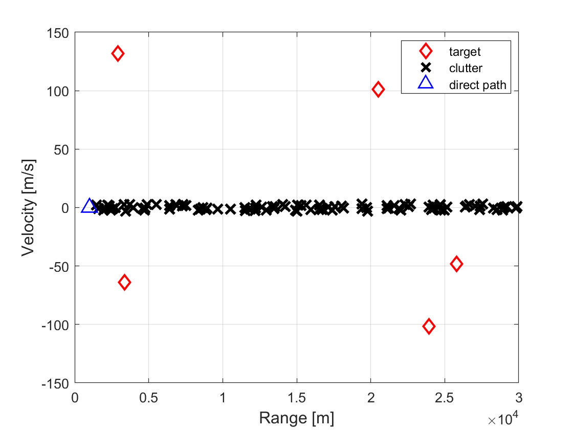
In the first test, we consider the scenario with multiple targets and clutters, and particularly set the number of targets to and the number of clutters to . Their velocity and range of these targets are shown in Fig. 1, where the red “” represents the targets, the black “” represents the clutters, and the blue “” represents the direct path. In this test, the targets and clutters are assumed to be point scatters which generated randomly in the range of ]km. Besides, the velocities of targets are within and the velocities of clutters are limited into . We assume that there is only one illuminator to transmit OFDM signal with a carrier frequency of GHZ. The length of OFDM symbol is and the length of the cyclic prefix is . We also assume that the number of subcarriers is , and the signal is divided into blocks for processing. In this test, all the algorithms are compiled with Matlab R2016a and run on a LENOVO laptop with one Intel Core Silver 4216 CPU Processor ( to GHz) and GB RAM.
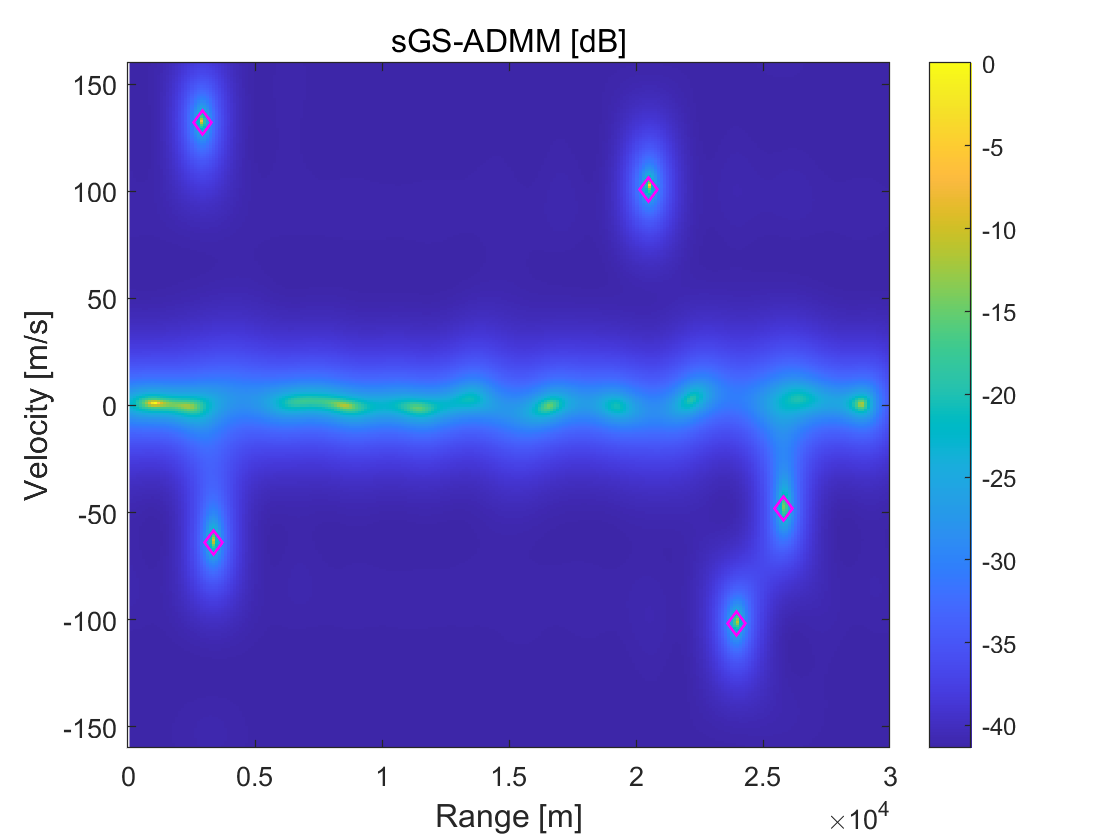
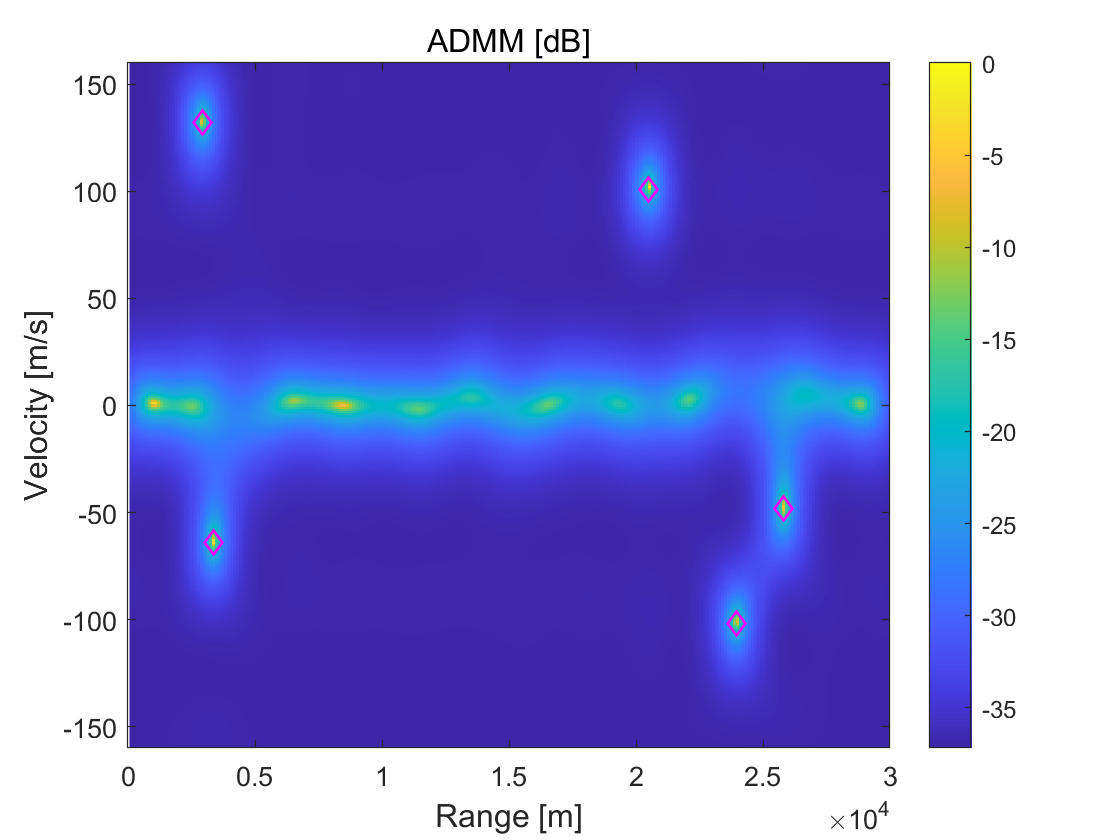
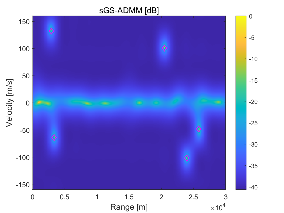
Taking the demodulation error into account, we employ the quadrature phase-shift keying (QPSK) to modulate, and use the bit-error-rates (BER) to measure demodulation error. In this test, we use sGS-ADMM and directly-extended ADMM, and then compare their performance for different BER from to with intervals. For each algorithm, the iterative process forcefully terminates when the number of iterations reaches , , and , to observe the algorithms’ performance within a fixed number of iterations. To get a distinct visual comparison, we plot the spectrum for estimation results derived from each algorithm in Figure 2. It can be clearly seen from this figure that there is no significant difference between sGS-ADMM and ADMM in the spectrum when BER is small. But, with the increases of BER, the estimations’ qualities produced by ADMM become lower and lower. At the case of BER, we see from the 2nd-column of Figure 2 that, many ghost peaks appeared in the spectrum, which may cause many difficulties to identify targets that lead to increasing the false alarms. In contrast, the spectrum displayed at the 1st-column is clearly accurate and “clean”, which shows that sGS-ADMM is able to detect these targets and does not degrade with the increases of BER.


4.2 Numerical performance comparisons
To evaluate the numerical efficiencies of each algorithm, we adopt the relative KKT residual to measure the estimation qualities associated with the problem (3.3). More precisely, the KKT residual, denoted by , is defined as
where
From optimization theory, we know that if only if is the solution of the problem (3.3). Hence, it is reasonable to stop the iterative process of both algorithms when is smaller than a given tolerance.
| step | BER | Time(s) | obj | n_tar | |
|---|---|---|---|---|---|
| (sGSAdA) | (sGSAdA) | (sGSAdA) | (sGSAdA) | ||
| 0 | 53.84 34.35 | 3.29e-041.29e-03 | 4.77e+03 7.22e+04 | 55 | |
| 100 | 0.02 | 56.32 36.81 | 3.20e-042.44e-03 | 5.25e+03 7.83e+04 | 55 |
| 0.04 | 54.89 36.46 | 3.49e-042.02e-03 | 6.00e+03 8.32e+04 | 55 | |
| 0.06 | 54.6636.45 | 3.68e-042.32e-03 | 5.80e+03 8.25e+04 | 55 | |
| 0.08 | 55.07 36.67 | 3.89e-042.53e-03 | 6.98e+03 8.99e+04 | 65 | |
| 0.1 | 55.07 36.70 | 4.17e-042.62e-03 | 7.71e+03 8.45e+04 | 56 | |
| 0 | 108.20 69.24 | 7.73e-053.48e-04 | 3.42e+03 7.28e+04 | 55 | |
| 200 | 0.02 | 112.17 83.68 | 8.07e-053.94e-04 | 3.90e+03 7.90e+04 | 55 |
| 0.04 | 109.79 72.38 | 8.45e-054.03e-04 | 4.60e+03 8.46e+04 | 55 | |
| 0.06 | 110.10 73.76 | 9.40e-054.13e-04 | 4.42e+03 8.37e+04 | 55 | |
| 0.08 | 110.25 73.45 | 9.00e-054.19e-04 | 5.60e+03 9.07e+04 | 55 | |
| 0.1 | 110.46 74.26 | 9.01e-054.95e-04 | 6.21e+03 8.20e+04 | 510 | |
| 0 | 162.20 103.47 | 3.68e-05 1.92e-04 | 2.89e+03 7.30e+04 | 55 | |
| 300 | 0.02 | 163.94 106.42 | 4.05e-052.05e-04 | 3.35e+03 7.93e+04 | 55 |
| 0.04 | 164.67 108.17 | 4.52e-052.20e-04 | 4.03e+03 8.52e+04 | 55 | |
| 0.06 | 165.34 110.52 | 4.62e-052.09e-04 | 3.86e+03 8.41e+04 | 55 | |
| 0.08 | 165.40 110.46 | 4.32e-052.13e-04 | 5.01e+03 9.03e+04 | 55 | |
| 0.1 | 166.29 112.09 | 4.59e-052.54e-04 | 5.60e+03 7.97e+04 | 520 |
To observe the convergence behavior of each algorithm numerically, we report the final objective values (obj), the number of identified targets (n_tar), the computing time required (Time), and the final KKT residuals () in the case of BER=. In this test, we only record these values of ‘n_star’, ‘Time’, ‘’, and ‘obj’ when the step (step) reaches , , and . These results are given in Table 1 where ‘sGSA’ and ‘dA’ are short for ‘sGS-ADMM’ and ‘ADMM’, respectively. From the last column, we see that both algorithms could successfully detect the number of targets, and from the last 2nd to 3rd columns, we see that sGS-ADMM outperforms ADMM in the sense that it derives higher quality solutions with lower final objective function values and smaller KKT residuals. But, we also see that sGS-ADMM always requires more computing time at each test case. I think that this phenomenon is not surprising because sGS-ADMM computes some variables twice per-iteration. To visibly see the performance of each algorithm, we plot the KKT residuals’ behavior versus the iteration in Figure 3. We see from this figure that, the KKT residuals generated by sGS-ADMM are always at the bottom, which indicates that sGS-ADMM decreases faster than ADMM. In conclusion, this test shows that both the objective-function values and the KKT residuals derived by sGS-ADMM decrease faster than that obtained by ADMM as iteration goes on.
To compare the numerical performance in a relatively fair way, we run both algorithms from the same point and terminate when their KKT residuals are smaller than a given tolerance, i.e.,
In this test, we choose the tolerance as Tol=, , and , respectively. Besides, we also force the iterative process to terminate when the number of iterations exceeds without achieving convergence. In this case, we say that the corresponding algorithm is failed. The detailed results derived by sGS-ADMM and ADMM with different BER values are reported in Table 2, in which the symbol ‘—’ represents that the algorithm fails to solve the corresponding problems.
| BER | tol | Time(s) | obj | Iter.NO | ||
|---|---|---|---|---|---|---|
| (sGSAdA) | (sGSAdA) | (sGSAdA) | (sGSAdA) | (sGSAdA) | (sGSAdA) | |
| 1.0e-03 | 15.4440.61 | 9.88e-049.67e-04 | 9.16e+037.23e+04 | 29114 | 55 | |
| 0 | 1.0e-04 | 95.32163.41 | 9.95e-059.97e-05 | 3.65e+037.30e+04 | 173467 | 55 |
| 1.0e-05 | 361.44342.50 | 9.99e-063.64e-05 | 2.15e+037.32e+04 | 663— | 55 | |
| 1.0e-03 | 14.9344.19 | 9.78e-049.85e-04 | 9.46e+047.80e+04 | 28126 | 55 | |
| 0.02 | 1.0e-04 | 95.46173.06 | 9.94e-059.98e-05 | 4.01e+037.92e+04 | 178483 | 55 |
| 1.0e-05 | 368.34349.95 | 9.98e-063.50e-05 | 2.53e+037.95e+04 | 673— | 55 | |
| 1.0e-03 | 14.8946.54 | 9.84e-049.81e-04 | 9.90e+038.23e+04 | 27130 | 55 | |
| 0.04 | 1.0e-04 | 99.69175.70 | 9.99e-059.98e-05 | 4.41e+038.41e+04 | 185500 | 55 |
| 1.0e-05 | 379.58351.64 | 9.98e-063.65e-05 | 3.01e+038.45e+04 | 694— | 55 | |
| 1.0e-03 | 11.2348.49 | 9.81e-049.84e-04 | 1.10e+048.40e+04 | 2132 | 25 | |
| 0.06 | 1.0e-04 | 106.24174.42 | 9.93e-059.99e-05 | 4.90e+038.52e+04 | 191479 | 55 |
| 1.0e-05 | 397.01362.69 | 9.99e-063.77e-05 | 3.45e+038.60e+04 | 719— | 55 | |
| 1.0e-03 | 11.2849.32 | 9.75e-049.80e-04 | 1.12e+048.73e+04 | 21135 | 15 | |
| 0.08 | 1.0e-04 | 109.69193.14 | 9.95e-059.97e-05 | 5.37e+038.59e+04 | 201525 | 56 |
| 1.0e-05 | 432.70368.50 | 9.97e-063.81e-05 | 3.69e+038.52e+04 | 798— | 55 | |
| 1.0e-03 | 9.0451.60 | 9.71e-049.87e-04 | 1.22e+049.06e+04 | 17141 | 115 | |
| 0.1 | 1.0e-04 | 107.59222.75 | 9.93e-059.98e-05 | 6.04e+038.51e+04 | 196602 | 522 |
| 1.0e-05 | 422.72368.05 | 9.98e-065.52e-05 | 3.98e+038.28e+04 | 776— | 530 |
We see from Table 2 that, sGS-ADMM is capable of solving all the problems in each tested case. However, ADMM still fails in the Tol= case although it is successful in the low- and mid-accuracy cases. In addition, we also notice that in the case that both algorithms succeeded, sGS-ADMM is still two times faster. The better performance of sGS-ADMM is consistent with the theoretical analysis aforementioned that the sGS has the ability to ensure convergence. While turning our attention to the final objective function values and the final KKT residuals, we find that these values derived by sGS-ADMM are always smaller than that by ADMM, which once again indicates that sGS-ADMM is a winner. At last, we see from the last column of this table that the number of targets identified by ADMM is not correct, especially in the case of BER, because the true number of moving targets is only . All in all, this test demonstrates that sGS-ADMM outputs a higher recognition rate and a lower false alarm rate. It should be noted that, since the targets are estimated by means of grid search but do not fall onto the discrete grids, the error related to the spacing of grids may exist invariably.
5 Conclusions and remarks
In recent literature, it was known that estimating the joint delay-Doppler of moving targets in OFDM passive radar can be described as an atomic-norm regularized convex minimization problem, or a SDP minimization problem. To solve this SDP problem, the directly-extended ADMM is not necessarily convergent although it performed well experimentally. To address this issue, in this paper, we skillfully partitioned the variables into two groups, i.e., and , and then used sGS at each group. One may think that this iteration form may lead to more computational costs thus leading to the algorithm being much more inefficient. But fortunately, the convergence result listed in Theorem 3.1 claimed that this algorithm should be more robust and efficient because the convergence property indeed reduced the number of iterations greatly. This claim was verified experimentally, that is, the sGS-ADMM worked successfully in most tested cases, derived higher-quality solutions, and run at least two times faster than ADMM.
There are some interesting topics that deserve further investigating. Firstly, the superior performance of sGS-ADMM is confirmed using some simulated data. But, its practical behaviors on real data sets need more testing. Secondly, we see that all the subproblems in sGS-ADMM are solved exactly. Hence, some strategies to solve these subproblems inexactly but has the ability to ensure convergence are also essential. Thirdly, we note that our approach is not able to locate the interesting targets accurately according to the velocity and range. Hence, the task of joint estimation of the velocity, range, and direction needs further investigation. At last, it is also an interesting topic to develop other efficient algorithms, such as algorithms for dual problem, to improve the performance of sGS-ADMM.
Acknowledges
The work of Y. Xiao is supported by the National Natural Science Foundation of China (Grants No. 11971149 and 12271217).
Conflict of interest
No potential conflict of interest was reported by the authors.
References
- Baczyk and Malanowski [2011] Baczyk, M., Malanowski, M., 2011. Reconstruction of the reference signal in dvb-t-based passive radar. International Journal of Electronics and Telecommunications .
- Bajwa et al. [2010] Bajwa, W.U., Haupt, J., Sayeed, A.M., Nowak, R., 2010. Compressed channel sensing: A new approach to estimating sparse multipath channels. Proceedings of the IEEE 98, 1058–1076.
- Berger et al. [2010] Berger, C.R., Demissie, B., Heckenbach, J., Willett, P., Zhou, S., 2010. Signal processing for passive radar using ofdm waveforms. IEEE Journal of Selected Topics in Signal Processing 4, 226–238.
- Bhaskar et al. [2013] Bhaskar, B.N., Tang, G., Recht, B., 2013. Atomic norm denoising with applications to line spectral estimation. IEEE Transactions on Signal Processing 61, 5987–5999.
- Candès and Fernandez-Granda [2013] Candès, E., Fernandez-Granda, C., 2013. Super-resolution from noisy data. Journal of Fourier Analysis and Applications 19, 1229–1254. doi:10.1007/s00041-013-9292-3. copyright: Copyright 2013 Elsevier B.V., All rights reserved.
- Candès and Fernandez-Granda [2014] Candès, E.J., Fernandez-Granda, C., 2014. Towards a mathematical theory of super-resolution. Communications on pure and applied Mathematics 67, 906–956.
- Cardinali et al. [2007] Cardinali, R., Colone, F., Ferretti, C., Lombardo, P., 2007. Comparison of clutter and multipath cancellation techniques for passive radar, in: 2007 IEEE Radar Conference, IEEE. pp. 469–474.
- Chandrasekaran et al. [2012] Chandrasekaran, V., Recht, B., Parrilo, P.A., Willsky, A.S., 2012. The convex geometry of linear inverse problems. Foundations of Computational mathematics 12, 805–849.
- Chen et al. [2016] Chen, C., He, B., Ye, Y., Yuan, X., 2016. The direct extension of admm for multi-block convex minimization problems is not necessarily convergent. Mathematical Programming 155, 57–79.
- Chen et al. [2017] Chen, L., Sun, D., Toh, K.C., 2017. An efficient inexact symmetric gauss–seidel based majorized admm for high-dimensional convex composite conic programming. Mathematical Programming 161, 237–270.
- Colone et al. [2006] Colone, F., Cardinali, R., Lombardo, P., 2006. Cancellation of clutter and multipath in passive radar using a sequential approach, in: 2006 IEEE Conference on Radar, IEEE. pp. 1–7.
- Colone et al. [2009] Colone, F., O’hagan, D., Lombardo, P., Baker, C., 2009. A multistage processing algorithm for disturbance removal and target detection in passive bistatic radar. IEEE Transactions on aerospace and electronic systems 45, 698–722.
- Ding and Xiao [2018] Ding, Y., Xiao, Y., 2018. Symmetric gauss–seidel technique-based alternating direction methods of multipliers for transform invariant low-rank textures problem. Journal of Mathematical Imaging and Vision 60, 1220–1230.
- Falcone et al. [2010] Falcone, P., Colone, F., Bongioanni, C., Lombardo, P., 2010. Experimental results for ofdm wifi-based passive bistatic radar, in: 2010 ieee radar conference, IEEE. pp. 516–521.
- Fazel et al. [2013] Fazel, M., Pong, T.K., Sun, D., Tseng, P., 2013. Hankel matrix rank minimization with applications to system identification and realization. SIAM Journal on Matrix Analysis and Applications 34, 946–977.
- Herman and Strohmer [2009] Herman, M.A., Strohmer, T., 2009. High-resolution radar via compressed sensing. IEEE transactions on signal processing 57, 2275–2284.
- Howland et al. [2005] Howland, P.E., Maksimiuk, D., Reitsma, G., 2005. Fm radio based bistatic radar. IEE proceedings-radar, sonar and navigation 152, 107–115.
- Hu et al. [2012] Hu, L., Shi, Z., Zhou, J., Fu, Q., 2012. Compressed sensing of complex sinusoids: An approach based on dictionary refinement. IEEE Transactions on Signal Processing 60, 3809–3822.
- Ketpan et al. [2015] Ketpan, W., Phonsri, S., Qian, R., Sellathurai, M., 2015. On the target detection in ofdm passive radar using music and compressive sensing, in: 2015 Sensor Signal Processing for Defence (SSPD), IEEE. pp. 1–5.
- Krim and Viberg [1996] Krim, H., Viberg, M., 1996. Two decades of array signal processing research: the parametric approach. IEEE signal processing magazine 13, 67–94.
- Li and Xiao [2018] Li, P., Xiao, Y., 2018. An efficient algorithm for sparse inverse covariance matrix estimation based on dual formulation. Computational Statistics & Data Analysis 128, 292–307.
- Li et al. [2016] Li, X., Sun, D., Toh, K.C., 2016. A schur complement based semi-proximal admm for convex quadratic conic programming and extensions. Mathematical Programming 155, 333–373.
- Li et al. [2019] Li, X., Sun, D., Toh, K.C., 2019. A block symmetric gauss–seidel decomposition theorem for convex composite quadratic programming and its applications. Mathematical Programming 175, 395–418.
- Moreau [1962] Moreau, J.J., 1962. Fonctions convexes duales et points proximaux dans un espace hilbertien. Comptes rendus hebdomadaires des séances de l’Académie des sciences 255, 2897–2899.
- Naha et al. [2014] Naha, A., Samanta, A.K., Routray, A., Deb, A.K., 2014. Determining autocorrelation matrix size and sampling frequency for music algorithm. IEEE Signal Processing Letters 22, 1016–1020.
- Palmer et al. [2012] Palmer, J.E., Harms, H.A., Searle, S.J., Davis, L., 2012. Dvb-t passive radar signal processing. IEEE transactions on Signal Processing 61, 2116–2126.
- Sen and Nehorai [2010] Sen, S., Nehorai, A., 2010. Adaptive ofdm radar for target detection in multipath scenarios. IEEE Transactions on Signal Processing 59, 78–90.
- Sun et al. [2015] Sun, D., Toh, K.C., Yang, L., 2015. A convergent 3-block semiproximal alternating direction method of multipliers for conic programming with 4-type constraints. SIAM journal on Optimization 25, 882–915.
- Tang et al. [2013] Tang, G., Bhaskar, B.N., Shah, P., Recht, B., 2013. Compressed sensing off the grid. IEEE transactions on information theory 59, 7465–7490.
- Tao et al. [2010] Tao, R., Wu, H., Shan, T., 2010. Direct-path suppression by spatial filtering in digital television terrestrial broadcasting-based passive radar. IET radar, sonar & navigation 4, 791–805.
- Yang and Xie [2016] Yang, Z., Xie, L., 2016. Exact joint sparse frequency recovery via optimization methods. IEEE Transactions on Signal Processing 64, 5145–5157.
- Yang et al. [2016] Yang, Z., Xie, L., Stoica, P., 2016. Vandermonde decomposition of multilevel toeplitz matrices with application to multidimensional super-resolution. IEEE Transactions on Information Theory 62, 3685–3701.
- Yang et al. [2012a] Yang, Z., Xie, L., Zhang, C., 2012a. Off-grid direction of arrival estimation using sparse bayesian inference. IEEE transactions on signal processing 61, 38–43.
- Yang et al. [2012b] Yang, Z., Zhang, C., Xie, L., 2012b. Robustly stable signal recovery in compressed sensing with structured matrix perturbation. IEEE Transactions on Signal Processing 60, 4658–4671.
- Zhang et al. [2015] Zhang, X., Li, H., Liu, J., Himed, B., 2015. Joint delay and doppler estimation for passive sensing with direct-path interference. IEEE Transactions on Signal Processing 64, 630–640.
- Zheng and Wang [2017] Zheng, L., Wang, X., 2017. Super-resolution delay-doppler estimation for ofdm passive radar. IEEE Transactions on Signal Processing 65, 2197–2210.