An evolutionary model of long tailed distributions in the social sciences

Consider a model populated initially by $N$ agents located in some space such as the sequence of real numbers. Depending on the phenomenon, each location is an abstract representation; it could refer to the city where a firm chooses to locate itself, but it could equally well refer to the product a consumer chooses, or the idea or fashion that a person follows.

The model proceeds in a series of steps. In each step, $n$ new agents enter the model, where the number $n$ is between 1 and $N$ and fixed as a parameter in each solution of the model. With probability $1-\mu$, an agent copies the choice of location from that of an existing agent within the previous m time steps, or else with probability $\mu$, the agent innovates by choosing a unique new location at random. In other words, the agent either copies an existing agent from the last $m$ steps, or chooses a new location.

Here we restrict our exploration to two key parameters of the model, $m$ and $\mu$, by choosing convenient values for $N$ and $n$. The ‘memory’ parameter $m$ determines the number of steps of the previous decisions of other agents over which an agent looks when making its decision. The ‘innovation’ parameter $\mu$ determines the fraction of the agents who decide to take a completely new decision rather than replicating one of the decisions made by other agents.

A specific version of the model, with $m=1$ (i.e., memory only of the immediately preceding step), is known in population genetics and physics 17 , 18 . For the special case of $n=N$ and $m=1$, analytical solutions demonstrate a power-law distribution 17 for $N\mu$ equal to or slightly greater than 1. For $m=1$ and $N\mu\ll 1$, this gradually converges on a winner-take-all distribution as $N\mu$ approaches zero.

The case where $m$ = all is a further special category of the model, where extinction or obsolescence does not occur. In this case, we can achieve different power law slopes by varying $n$ and $\mu$. Figure 1 shows, for example, that we can match the B-A preferential attachment model 7 , obtaining a power law exponent $\alpha\sim 3$ over the entire distribution, by using $m=all$ with $N=1,n=10,t=20,000$, and $\mu=0.6$.

For socio-cultural phenomena, however, we expect memory to be limited, and thus $m$ in general to take values below the special case of ‘all’. So while we define the model to allow $m$ to take any value between 1 and all, we explore here a limited range, from $m=1$ to $m=100$ time steps of limited memory. The combined effect of varying $m$ along with varying the innovation parameter $\mu$ generates both a wide range of right-skew distributional forms and turnover of rankings of locations within those distributions. Considerable anthropological and socio-economic evidence exists 19 , 20 , 21 , 22 , 23 on the plausible values for $\mu$ being no greater than 0.1.

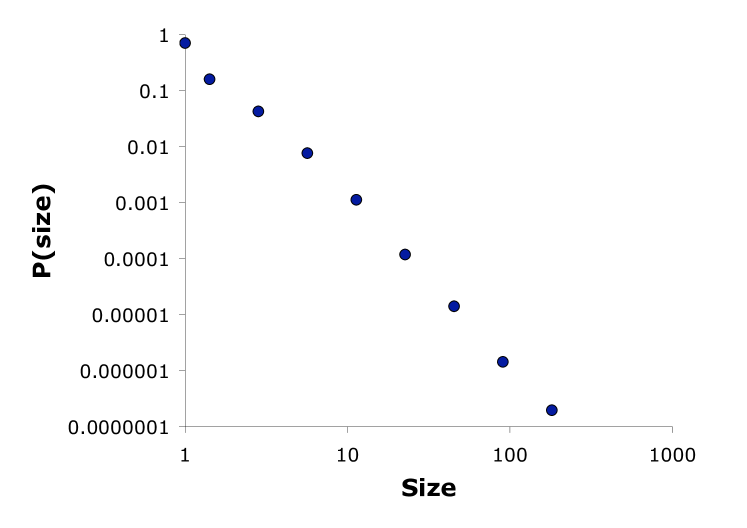
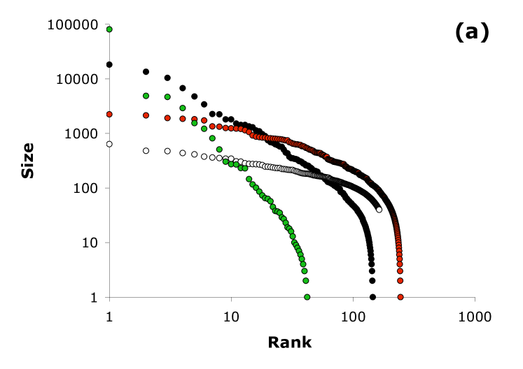
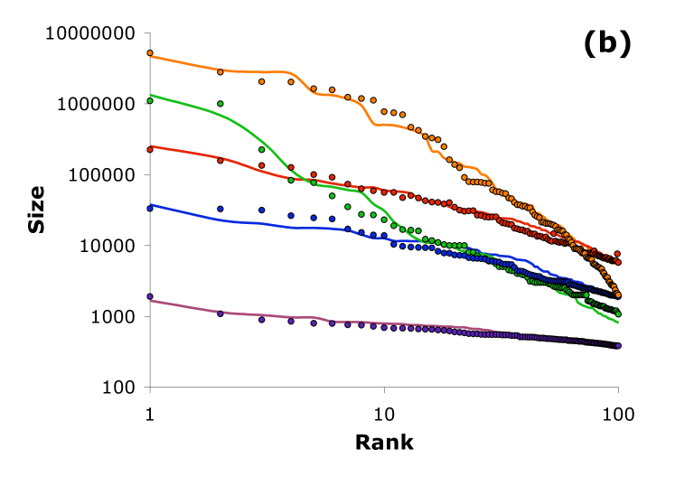
Figure 2a plots typical solutions of the model using acceptable values of $\mu$, while varying $m$ (holding $N=1000$, $n=100$ and showing the results at time step 1000). Aside from the selected results shown in this figure, the model produces additional results ranging from a winner-take-all outcome, to a power law over the entire distribution (exponent $\alpha\sim 1.5$), to a power law fitted to the tail of varying exponent. Figure 2b illustrates how the model parameters can be selected so that the results match real-world right-skew distributions, such as religions, website subscriptions, word use, names, and author citations.

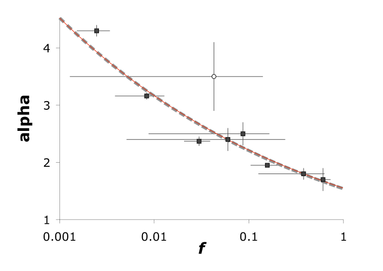
Table 1 lists power law tail exponents $\alpha$ for various recently collated social data sets 1 , 2 along with the fraction $f$($=n_{tail}/n$) of total observations in the tail. A striking, and previously unreported, feature of these estimates is the relationship between $\alpha$ and $f$, where these data reveal a clear inverse correlation. The smaller the fraction $f$ of the distribution best-fit to a power law tail 24 , the larger the exponent $\alpha$ of that tail. The least-squares fit is $\alpha\cong 1.54f^{-0.156}$ ($r^{2}=0.952$).

Figure 3 plots this relationship in the empirical data along with the least squares fit using the model, as solved 100 times, for each of $\mu=$ 0.05, 0.06 and 0.07, with $m=30$ in each case (and $N=1000$, $n=100$, $t=1,000$). The results show $\alpha\cong 1.56f^{-0.155}$ ($r^{2}=0.975$), very similar to the data-based relationship.

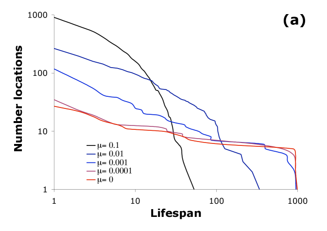
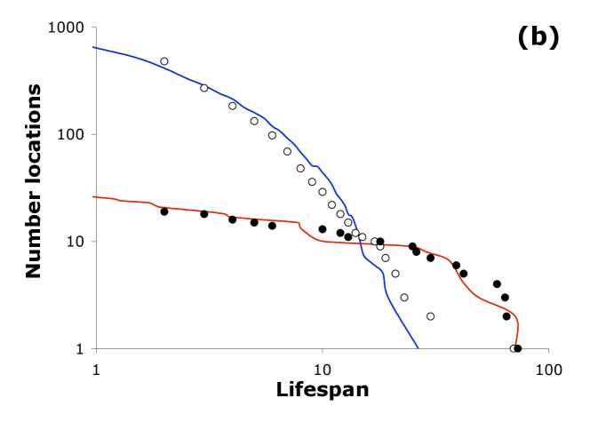
The model also produces continual turnover through time for any given distribution as demonstrated by the distributions of lifespans within ranked lists as in Figure 4a. This resembles the lifespans of real world social and economic fat-tail distributions in Figure 4b. The memory parameter $m$ again expands the power of the model. Although turnover has already been demonstrated 17 for the special case $m=1$, different values of m are needed to account for empirically observed turnover (Supplementary Information shows distributions generated for increasing memory $m$ with order of magnitude changes in the value of $\mu$).

The model we have presented can generate not only a wide range of long-tailed distributions but a constant turnover of the constituent agents within any given overall rank-size distribution. It is also able to replicate a newly-identified empirical relationship whereby the power law exponent increases as the proportion of data in the tail falls.

The model is quite general, despite using only two parameters. Varying the parameter values can yield a range of distributions, such as a power law over the whole sample, a power law only in the tail, and a winner-take-all outcome. Since the parameter $m$ represents memory and $\mu$ represents innovation in modelled decision-making, the real-world relationship between $\alpha$ and $f$ in Figure 3 may result from a variation in related parameters among the different contexts of human decision-making. We conjecture that the continuous relationship observed in Figure 3 suggests that socio-economic power law distributions may form a continuum resulting from a generalised process with limited memory. In contrast to the special $m=all$ case (Figure 1), when model runs with limited memory yield a power law over the entire distribution ($f=1$), it is only with exponent $\alpha$ close to 1.5 (Figure 3).

This combination of results makes this model unique among the many alternatives that can produce power laws. The most commonly proposed processes such as preferential attachment, proportionate effect based on Gibrat’s principle, the ‘Matthew effect’ and the Yule process 1 , 2 , 14 , 25 , 26 , produce power laws from the positive feedback introduced by interactions between individual agents. But these ‘rich get richer’ models have not been able to account for flux in the constituents of the ranked distribution 27 , either when growth is one of strict preferential attachment or even when growth is proportionate to a stochastic rate independent of size 28 . Even though “dynamical problems lie at the forefront” of network science 16 , in most network models, existing connections affect future connections such that change does not occur naturally, but only with imposed modifications.

Social scientists have been critical of modelling social and economic data by mapping onto known phenomena in physics without considering realistic behavioural motivations of the agents 12 , 29 , 30 . As a step in this direction, our model captures two fundamental motivations, the imitation of others and novelty in invention.

Compared to similar, less flexible versions of this model 15 , a crucial new variable appears to be the memory $m$, which reflects different time frames to which agents will refer in different contexts. In terms of pure fashion markets such as popular music for example Salganik2006 , agents take into account only the most recent decisions of others and hardly ever those of several months or even weeks ago. However in choosing where to locate geographically, for example, a firm or a person in a city will implicitly be using information from many previous time steps with respect to the decisions made by others.

Generating a range of long-tailed distributions with dynamic turnover, these features distinguish this model from the standard socio-economic science model of individual rational behaviour where social influence is the exception to the rule (as in, for example, ‘irrational’ stock market bubbles or real estate crises). With its unrealistic psychological assumptions Kahneman2003 and inconsistencies with experimental results Smith2003 , the standard model suffers from a neglect of social influence, even in its modern form which permits, for example, asymmetry in the amount of information possessed by different agents Akerlof1970 , Stiglitz2002 , the cost of gathering information Stigler1961 , and imperfections in gathering and processing information 3 .

Social influence is arguably ubiquitous among the human species DunbarShultz2007 . In fact, rather than the agent’s cost-benefit analysis that has served as a null hypothesis for rationality for over a century, an alternative is that each agent uses (consciously or not) the decisions of others as a basis for his or her own decisions.

The social-influence model we have presented allows choices among multiple possible alternatives, which rise and fall in relative popularity over time, rather than binary, ‘either-or’ decisions. This is truly reflective of human interactions such as the choice of a popular name for a child, the citation of an academic paper, or movement to a city where others have chosen to live. Indeed, these phenomena are inherently defined by the past decisions of others, without which there would be no cities, familiar names, or popular culture.

Batty was partially supported by the EPSRC Spatially Embedded Complex Systems Engineering Consortium (EP/C513703/1). Amy Heineike of Volterra provided programming support.

References

- [1] Newman MEJ (2005) Power laws, Pareto distributions and Zipf s law. Contemporary Physics 46: 323-351.
- [2] Clauset A, Shalizi CR, Newman MEJ (2007) ower-law distributions in empirical data. arXiv 07061062v1.
- [3] H.A. Simon (1955) A behavioral model of rational choice. Quarterly J. Economics 59: 99-118 .
- [4] G.K. Zipf (1949) Human Behavior and the Principle of Least Effort (Addison Wesley, Cambridge, MA)
- [5] Price DJD (1965) Networks of scientific papers. Science 149: 510-512.
- [6] Huberman BA, Adamic AL (1999) Growth dynamics of the World-Wide Web. Nature 401: 131.
- [7] Barabási AL, Albert R (1999) Emergence of scaling in random networks. Science 286: 509-512.
- [8] Redner, S (1998) How popular is your paper? An empirical study of the citation distribution. European Physical Journal B 4: 131-134.
- [9] Liljeros, F, Edling, CR, Amaral LAN, Stanley HE, Aberg Y (2001) The web of human sexual contacts. Nature 411: 907-908.
- [10] Axtell RL (2001) Zipf distribution of U.S. firm sizes. Science 293: 1818-1820.
- [11] Ormerod P (2006) Why Most Things Fail: Evolution, Extinction and Economics (Pantheon Books, New York).
- [12] Borgatti SP, Mehra A, Brass DJ (2009) Network analysis in the social sciences. Science 323: 892-895.
- [13] Laherrère J, Sornette D (1998) Stretched exponential distributions in nature and economy: ‘fat tails’ with characteristic scales. European Physical Journal B 2: 525-539.
- [14] Batty M (2006) Rank clocks. Nature 44: 592-596.
- [15] Bentley RA, Lipo CP, Herzog HA, Hahn MW (2007) Regular rates of popular culture change reflect random copying. Evolution and Human Behaviour 28: 151-158.
- [16] Newman MEJ, Barabási A-L, Watts DJ (2005) The Structure and Dynamics of Networks (Princeton University Press, Princeton, NJ).
- [17] Evans TS (2007) Exact solutions for network rewiring models. European Physical Journal B 56: 65-69.
- [18] Gillespie JH (2004) Population Genetics (Johns Hopkins University Press, Baltimore, MD)
- [19] Eerkens JW (2000) Practice makes within 5% of perfect. Current Anthropology 41: 663-668.
- [20] Diederen P, van Meijl H, Wolters A, Bijak K (2003) Innovation adoption in agriculture. Cahiers d’économie et Sociologie Rurales 67: 30-50.
- [21] Srinivasan V, Mason CH (1986) Nonlinear least squares estimation of new product diffusion models. Marketing Science 5: 169-178.
- [22] Larsen ON (1961) Innovators and early adopters of television. Sociological Inquiry 32: 16-33.
- [23] Rogers EM (1962) Diffusion of Innovations (Free Press, New York)
- [24] Omitting one outlier (email address book sizes). This is not simply a statistical outlier, but the process underlying it may violate our definition of ‘socio-cultural’, in that many such lists are generated by automated computer algorithms.
- [25] Yule GU (1925) A mathematical theory of evolution based on the conclusions of Dr. J. C. Willis. Phil. Trans. R. Soc. London B 213: 21-87.
- [26] Simon HA (1955) On a class of skew distribution functions. Biometrica 42: 425-440.
- [27] Batty M (2008) The size, scale, and shape of cities. Science 319: 769-771.
- [28] Gibrat R (1931) Les Inégalités Économiques (Librarie du Recueil Sirey, Paris.
- [29] Gallegati M, Keen S, Lux T, Ormerod P (2006) Worrying trends in econophysics. Physica A 370: 1-6.
- [30] Bentley RA, Shennan SJ (2005) Random copying and cultural evolution. Science 309: 877-879.
- [31] Salganik MJ, Dodds PS and Watts DJ (2006) Experimental study of inequality and unpredictability in an arti cial cultural market. it Science 311: 854-856.
- [32] Kahneman D (2003) Maps of bounded rationality: psychology for behavioral economics. Am. Economic Rev. 93: 1449-1475.
- [33] Smith VL (2003) Constructivist and ecological rationality in economics. Am. Economic Rev. 93: 465-508.
- [34] Akerlof GA (1970) The market for ‘lemons’: Quality uncertainty and the market mechanism.Quarterly J. Economics 84: 488-500.
- [35] Stiglitz JE (2002) Information and the change in the paradigm in economics. Am. Economic Rev. 92: 460-501.
- [36] Stigler GJ (1961) The economics of information. J. Political Economy 69: 213-225.
- [37] Dunbar RIM, Shultz S (2007) Evolution in the social brain. Science 317: 1344-1347.
- [38] Data sources: Male baby names from www.census.gov, RSS feeds from radio.xmlstoragesystem.com/rcsPublic, English words from www.bckelk.ukfsn.org /words/uk1000n.html, cited economists from www.in-cites.com, and religious adherents from www.adherents.com.
- [39] Data: www.theofficialcharts.com.
- [40] Data: www.ssa.gov/OACT/babynames