An exponential integrator multicontinuum homogenization method for fractional diffusion problem with multiscale coefficients

Yifei Gao, Yating Wang, Wing Tat Leung, Zhengya Yang

An exponential integrator multicontinuum homogenization method for fractional diffusion problem with multiscale coefficients

Yifei Gao, Yating Wang, Wing Tat Leung, Zhengya Yang

Abstract

In this paper, we present a robust and fully discretized method for solving the time fractional diffusion equation with high-contrast multiscale coefficients. We establish the homogenized equation in a coarse mesh using a multicontinuum approach and employ the exponential integrator method for time discretization. The multicontinuum upscaled model captures the physical characteristics of the solution for the high-contrast multiscale problem, including averages and gradient effects in each continuum at the coarse scale. We use the exponential integration method to address the nonlocality induced by the time fractional derivative and the stiffness from the multiscale coefficients in the semi-discretized problem. Convergence analysis of the numerical scheme is provided, along with illustrative numerical examples. Our results demonstrate the accuracy, efficiency, and improved stability for varying order of fractional derivatives.

1 Introduction

Time fractional diffusion equations are extensively utilized to describe the subdiffusion phenomena in porous media. The fractional operators can be a useful way to include memory in the dynamical process. It is modeled through fractional order derivatives carries information about its present as well as past states. Due to the highly heterogeneous nature of the underlying media, the multiscale coefficients in these equations often exhibit high-contrast and nonlocality characteristics. Such features are prevalent in various applications, including composite materials, groundwater modeling, and reservoir simulations. It is essential to consider the heterogeneities of porous media and the phenomena of subdiffusion and we could achieve more accurate modeling in practical applications. However, the time fractional derivative and multiscale feature of the semilinear problems pose significant challenges in simulation.

Indeed, the presence of high-contrast/multicontinuum fields leads to the lack of smoothness in the exact solution, and the fractional order of the time derivative results in long-persistent memory. Thus making it difficult to construct accurate and computationally efficient numerical schemes. To capture all scale information of the solution, small mesh size for the spatial discretization is usually needed to ensure accuracy. And the stiffness arising from the multiscale coefficients requires the use of very small time steps to meet stability requirements using conventional explicit temporal discretization methods. When the order of the time fractional derivative reaches zero, some numerical schemes turns out to be unstable due to the singularity. The nonlocality of the fractional derivative also makes long-time simulation prohibitive.

In previous works, many developed multiscale models have been proposed. These multiscale approaches include multisacle finite element methods (MsFEM) [1, 2, 3], mixed MsFEM [4], numerical homogenized methods [5, 6, 7], numerical upsacling methods [8, 9, 10], generalized multiscale finite element methods (GMsFEM) [11, 12, 13], localized orthogonal decomposition (LOD) [14], constraint energy minimizing GMsFEM (CEM-GMsFEM) [15] and nonlocal multicontinuum method (NLMC) [16], to name a few. Recently, the multicontinuum model is proposed based on the framework of multicontinuum homogenization [17, 18]. It can capture the property of the solution with multiple quantities. The main idea is to represent the solution via averages and its gradient effects in each continua. For diffusion equations, some previous works have been developed [19, 20, 21]. Researchers have developed many methods to discretize the time fractional derivative. The L1 scheme is one of the well known time stepping schemes that uses piecewise linear approximation on each time step [22, 23, 24, 25]. To overcome the difficulties caused by the stiffness and semilinear term, there has been a renewed interest in using exponential integrator methods [26, 27, 28, 29, 19].

In this work, we propose a robust and accurate scheme to solve the high-contrast time fractional diffusion equation. We derive the semi-discretized coarse scale model based on the multicontinuum homogenization method. Then we adopt the exponential integrator method for temporal discretization to ensure stability and efficiency for the semilinear problem. The convergence of our proposed approach is presented. The main contributions of this work are the following.

•

We derive time fractional multicontinuum upscaled model and analyze its convergence.
•

We then adopt exponential integrator for temporal discretization and compare it with L1 scheme for semilinear time fractional diffusion equation. We present the convergence result.
•

We perform some numerical experiments to show the accuracy and stability of our methods. We observe that the proposed method is more stable than L1 scheme when the fractional order is small for the high-contrast subdiffusion equation.

The paper is organized as follows. In Section 2, we will introduce the problem setting and some preliminary definitions for the latter discussion. In Section 3, we will discuss the spatial discretization and present the analysis of semi-discretized problems. We discuss the temporal discretization and present the analysis of full-discretized scheme in Section 4. We present numerical results in Section 5 and give concluding remarks in the final section.

2 Problem setup

We focus on the following time fractional diffusion equation

\left\{\begin{aligned} {}^{C}_{0}{D}_{t}^{\alpha}u-\mathrm{div}(\kappa\nabla u)&=f(u)\ &\mathrm{in}\,&\Omega\times\bigl{(}0,T\bigr{]},\\ u(t,x)&=0\ &\mathrm{on}\,&\partial\Omega\times\bigl{(}0,T\bigr{]},\\ u(0,x)&=u_{0}(x)\ &\mathrm{in}\,&\Omega,\end{aligned}\right.

(1)

where ${}^{C}_{0}{D}_{t}^{\alpha}u$ is defined as the Caputo fractional derivatives of order $\alpha\in(0,1)$ [24]

{}^{C}_{0}{D}_{t}^{\alpha}u(x,t)=\frac{1}{\Gamma(1-\alpha)}\int_{0}^{t}\frac{\partial u(x,s)}{\partial s}\frac{1}{(t-s)^{\alpha}}\,\mathrm{d}s.

(2)

We assume that $\kappa$ is a high-contrast heterogeneous permeability field. It is uniformly positive and bounded in $\Omega,\ \,\mathrm{i}.\mathrm{e}.\,\ \exists\,0<\kappa_{0}<\kappa_{1}<\infty$ such that $\kappa_{0}\leq\kappa\leq\kappa_{1},\ \mathrm{in}\,\overline{\Omega}$ .

There are three distinct scales which is highly related to our proposed homogenization method:

•

The physical microscopic scale $\varepsilon$ , which represents the behavior and microscopic structure with high-contrast;
•

The computational upscaling scale $H$ , where the homogenized problem is posed;
•

The observing scale $h$ , where the multicontinuum quantities, such as local averages of the multiscale solution, are defined.

These scale parameter satisfies $\varepsilon\leq h<H$ .

We start with the weak form of (1): find $u\in H_{0}^{1}(\Omega)$ satisfying

\bigl{(}\,_{0}^{C}D_{t}^{\alpha}u,v\,\bigr{)}+a_{\varepsilon}(u,v)=(f,v)\quad\forall\,v\in H_{0}^{1}(\Omega),

(3)

where $(\cdot,\cdot)$ represent the standard $L^{2}$ inner product and $a_{\varepsilon}(\cdot,\cdot)$ is defined as $a_{\varepsilon}(u,v)=\int_{\Omega}\kappa\nabla u\cdot\nabla v$ . Let $\omega_{i}$ be disjoint and $\Omega=\bigcup\limits_{i}\omega_{i}$ . We then extent the definition of the bilinear operator $a_{\varepsilon}(\cdot,\cdot)$ to $H^{1}(\Omega)$ as follows

a_{\varepsilon}(u,v)=\sum\limits_{i}\int_{\omega_{i}}\kappa\nabla u|_{\omega_{i}}\cdot\nabla v|_{\omega_{i}}.

Moreover, we define $\bigl{\lVert}\,u\,\bigr{\rVert}_{a(\omega)}\coloneqq\bigl{(}\,\int_{\omega}\kappa\bigl{\lvert}\,\nabla u\,\bigr{\rvert}^{2}\,\bigr{)}^{\frac{1}{2}}$ and denote $\bigl{\lVert}\,\cdot\,\bigr{\rVert}_{a}=\bigl{\lVert}\,\cdot\,\bigr{\rVert}_{a(\Omega)}$ . Let $\bigl{\lVert}\,\cdot\,\bigr{\rVert}$ be the standard $L^{2}$ norm of the domain $\Omega$ . We also assume the domain $\Omega$ can be divided into two subregions $\Omega=\Omega_{0}\cup\Omega_{1}$ . The subdomains $\Omega_{0}$ and $\Omega_{1}$ represent the region with high and low conductivity respectively.

3 Time fractional multicontinuum upscaling model

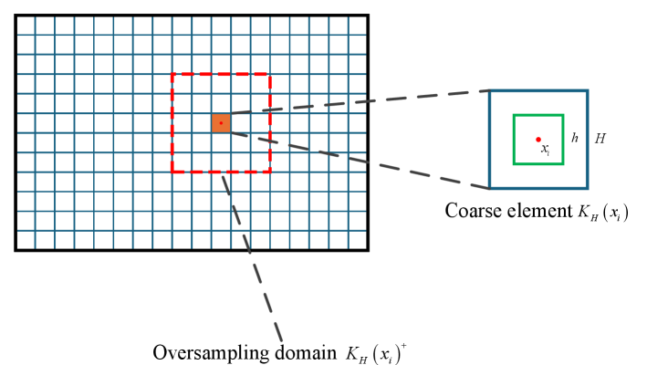
In this section, we would like to derive the multicontinuum upscaling model. We start with the construction of local basis and present the related convergence analysis. The computational domain $\Omega$ can be partitioned with respect to different scales. Given $z\in[0,H]^{d}$ ( $d=2,3$ ), we define a rectangular partition $\mathcal{T}_{H}(z)$ with mesh size $H$

\mathcal{T}_{H}(z)=\bigl{\{}\,K\subset\Omega\mid K=x_{i}+(-\frac{H}{2},\frac{H}{2})^{d}\cap\Omega,\frac{x_{i}-z}{H}\in\mathbb{Z}^{d}\,\bigr{\}},\ i=1,2,\cdots

For each coarse block $K_{H}(x_{i})=K_{z,H}(x_{i})\coloneqq x_{i}+(-\frac{H}{2},\frac{H}{2})^{d}\cap\Omega\in\mathcal{T}_{H}(z)$ , we can separate the element into two subregions, $K_{H,0}(x_{i})=K_{H}(x_{i})\cap\Omega_{0},\ K_{H,1}(x_{i})=K_{H}(x_{i})\cap\Omega_{1}$ . The index set is defined as $I_{H}=I_{z,H}=\bigl{\{}\,x_{i}\mid K_{H}(x_{i})\in\mathcal{T}_{H}(z)\,\bigr{\}}$ , it contains all of the center points of the coarse elements in the partition $\mathcal{T}_{H}(z)$ . Similarly, we can define the other partition $\mathcal{T}_{h}$ and its index set $I_{h}$ with the mesh size $h$ . An illustration of the mesh grid is shown in Figure 1.

Refer to caption — Fig. 1: The fine grid, coarse grid $K_{H}(x_{i})$ , oversampling domain $K_{H}(x_{i})^{+}$ .

3.1 Construction of local problems

In this subsection, we construct the local problems for the multicontinuum upscaling model. We define the auxiliary basis $\psi_{i,j}=\chi_{K_{H}(x_{i})}=1\quad\mathrm{in\ continuum\ }i$ and $\ 0\quad\mathrm{otherwise}$ . Based on CEM-GMsFEM/NLMC, the global basis functions $\varphi_{l,j}\in H_{0}^{1}(\Omega)\quad j=0,1$ can be obtained by solving the constrained energy minimization problems

	$\displaystyle a_{\varepsilon}(\varphi_{l,i},v)+\sum\limits_{x_{k}\in I_{z,h}}\sum\limits_{j=0,1}\eta^{k,j}(\psi_{k,j},v)$	$\displaystyle=0,$		(4)
	$\displaystyle(\varphi_{l,i},\psi_{k,j})$	$\displaystyle=\delta_{ij}\delta_{lk}\int_{\Omega}\psi_{k,j},$		(4)

where $\eta^{k,j}$ represents the energy constraint constant. We set the global multiscale space as $V_{glo,h}=\mathop{\mathrm{span}}_{l,j}\bigl{\{}\,\varphi_{l,j}\,\bigr{\}}=\bigl{\{}\,v\in H_{0}^{1}(\Omega)\mid v=\sum_{l,j}v_{l,j}\varphi_{l,j}\,\bigr{\}}$ . The convergence of the CEM-GMsFEM method with global basis is as follows [16], and it will be used in our latter discussions.

Lemma 3.1.

Let $f\in L^{2}(\Omega)$ and $u_{glo,h}\in V_{glo,h}$ be the solution of $a_{\varepsilon}(u_{glo,h},v)=(f,v)\quad\forall\,v\in V_{glo,h}$ . We have $\int_{\Omega}(u_{glo,h}-u)\psi_{k,j}=0\quad\forall\,k,j$ and $\bigl{\lVert}\,u_{glo,h}-u\,\bigr{\rVert}_{a}=O(h)$ .

We can denote $u_{glo,h}=\sum_{x_{l}\in I_{z}}U_{l,i}\,\varphi_{l,i}$ where the coefficients $U_{l,i}=\dfrac{(u,\psi_{l,i})}{\int_{\Omega}\psi_{l,i}}$ are the local average of the solution $u$ in the coarse elements $K_{H}(x_{l})$ .

In this work, we would like to introduce a time fractional multicontinuum model based on [17, 18], where the local problems correspond to the average and the gradient effect of the solution. To be more specific, to derive the homogenized equation on coarse scale, we first need to find $\phi_{i}$ and $\phi_{i}^{m}$ in $i$ -th coarse region from the following two cell problems with constraints

\left\{\begin{aligned} \int_{K_{H}^{+}(x)}\kappa(y)\nabla_{y}\phi_{i}(x,y)\nabla_{y}v&=\sum\limits_{k=0,1}\sum\limits_{x_{j}\in I_{H}\cap K_{H}(x)^{+}}d_{jk}\bigl{(}\,\psi_{k}(x_{j},y),v\,\bigr{)},\\ \bigl{(}\,\phi_{i}(x,y),\psi_{k}(x_{j},y)\,\bigr{)}&=\delta_{ki}\int_{K_{H}(x)^{+}}\psi_{k}(x_{j},y)\quad\forall\,x_{j}\in I_{H}\cap K_{H}(x)^{+},\end{aligned}\right.

(5)

\left\{\begin{aligned} \int_{K_{H}^{+}(x)}\kappa(y)\nabla_{y}\phi_{i}^{m}(x,y)\nabla_{y}v&=\sum\limits_{k=0,1}\sum\limits_{x_{j}\in I_{H}\cap K_{H}(x)^{+}}d_{jk}\bigl{(}\,\psi_{k}(x_{j},y),v\,\bigr{)},\\ \bigl{(}\,\phi_{i}^{m}(x,y),\psi_{k}(x_{j},y)\,\bigr{)}&=\delta_{ki}\int_{K_{H}(x)^{+}}(y^{m}-c_{x}^{(l)})\psi_{k}(x_{j},y)\quad\forall\,x_{j}\in I_{H}\cap K_{H}(x)^{+},\end{aligned}\right.

(6)

where $K_{H}(x)^{+}$ is the oversampling domain which enrich $K_{H}(x)$ by $k\ h$ -layer, $y^{(m)}$ is the $l$ -th coordinate of $y\in\mathbb{R}^{d}$ and $c_{x}^{(m)}$ are some constants such that $\int_{K_{H}(x)}(y^{(m)}-c_{x}^{(m)})=0$ . The solution $\phi_{i}$ of the cell problem (5) describe the averages in each continua while the solution $\phi_{i}^{m}$ of (6) represents the linear basis function. The upsacling model with the following scaling holds

\bigl{\lVert}\,\phi_{i}\,\bigr{\rVert}=O(1),\ \bigl{\lVert}\,\nabla\phi_{i}\,\bigr{\rVert}=O(\frac{1}{\varepsilon}),\ \bigl{\lVert}\,\phi_{i}^{m}\,\bigr{\rVert}=O(\varepsilon),\ \bigl{\lVert}\,\nabla\phi_{i}^{m}\,\bigr{\rVert}=O(1).

(7)

3.2 Multi-continuum upscaling model

Now we present the construction of the multiscale upscaling model. We assume that in each coarse block $K_{H}(x)$ , the solution $u$ could be approximated by $u=\phi_{i}U_{i}+\phi_{i}^{m}\nabla_{m}U_{i}$ , where $U_{i}$ can be view as a limit of $\frac{\int_{K_{H}(x)}u\psi_{i}}{\int_{K_{H}(x)}\psi_{i}}$ as the block size goes to zero. It represents the average solution in $i$ -th continua. With this expression of $u$ , we can write

\int_{K_{H}(x)}\kappa\nabla u\cdot\nabla v=\int_{K_{H}(x)}\kappa\nabla(\phi_{i}U_{i})\cdot\nabla v+\int_{K_{H}(x)}\kappa\nabla(\phi_{i}^{m}\nabla_{m}U_{i})\cdot\nabla v.

(8)

Approximately, we have

	$\displaystyle\int_{K_{H}(x)}\kappa\nabla(\phi_{i}U_{i})\cdot\nabla v$	$\displaystyle=\int_{K_{H}(x)}\kappa(\nabla\phi_{i})U_{i}\cdot\nabla v=U_{i}(x)\int_{K_{H}(x)}\kappa\nabla\phi_{i}\cdot\nabla v,$
	$\displaystyle\int_{K_{H}(x)}\kappa\nabla(\phi_{i}^{m}\nabla_{m}U_{i})\cdot\nabla v$	$\displaystyle=\int_{K_{H}(x)}\kappa\nabla(\phi_{i}^{m})\nabla_{m}U_{i}\cdot\nabla v=\nabla_{m}U_{i}(x)\int_{K_{H}(x)}\kappa\nabla\phi_{i}^{m}\cdot\nabla v.$

We take $v=\phi_{j}V_{j}+\phi_{j}^{n}\nabla_{n}V_{j}$ . Substitute the above equations into (8), we obtain

		$\displaystyle\int_{K_{H}(x)}\kappa\nabla u\cdot\nabla v=\int_{K_{H}(x)}\kappa\nabla(\phi_{i}U_{i})\cdot\nabla v+\int_{K_{H}(x)}\kappa\nabla(\phi_{i}^{m}\nabla_{m}U_{i})\cdot\nabla v$
	$\displaystyle=$	$\displaystyle\nabla_{m}U_{i}(x)\nabla_{n}V_{j}(x)\int_{K_{H}(x)}\kappa\nabla\phi_{i}^{m}\cdot\nabla\phi_{j}^{n}+\nabla_{m}U_{i}(x)V_{j}(x)\int_{K_{H}(x)}\kappa\nabla\phi_{i}^{m}\cdot\nabla\phi_{j}$
		$\displaystyle+U_{i}(x)\nabla_{n}V_{j}(x)\int_{K_{H}(x)}\kappa\nabla\phi_{i}\cdot\nabla\phi_{j}^{n}+U_{i}(x)V_{j}(x)\int_{K_{H}(x)}\kappa\nabla\phi_{i}\cdot\nabla\phi_{j}.$

Denote by $\alpha_{ij}^{mn}=\int_{K_{H}(x)}\kappa\nabla\phi_{i}^{m}\cdot\nabla\phi_{j}^{n},\ \beta_{ij}^{m}=\int_{K_{H}(x)}\kappa\nabla\phi_{i}^{m}\cdot\nabla\phi_{j},\ \gamma_{ij}=\int_{K_{H}(x)}\kappa\nabla\phi_{i}\cdot\nabla\phi_{j}$ . The above equations can be simplified as

\int_{K_{H}(x)}\kappa\nabla u\cdot\nabla v=\nabla_{m}U_{i}\alpha_{ij}^{mn}\nabla_{n}V_{j}+\nabla_{m}U_{i}\beta_{ij}^{m}V_{j}+U_{i}\beta_{ji}^{n}\nabla_{n}V_{j}+U_{i}\gamma_{ij}V_{j}.

Assume the cell problems do not depend on time $t$ , for the time fractional problem (3), we have ${}^{C}_{0}{D}_{t}^{\alpha}u=\phi_{i}\,{}_{0}^{C}D_{t}^{\alpha}U_{i}+\phi_{i}^{m}\,{}_{0}^{C}D_{t}^{\alpha}\nabla_{m}U_{i}$

	$\displaystyle\int_{K_{H}(x)}\,{}_{0}^{C}D_{t}^{\alpha}u\,v=$	$\displaystyle{}_{0}^{C}D_{t}^{\alpha}U_{i}V_{j}\int_{K_{H}(x)}\phi_{i}\phi_{j}+\,_{0}^{C}D_{t}^{\alpha}\nabla_{m}U_{i}V_{j}\int_{K_{H}(x)}\phi_{i}^{m}\phi_{j}$
		$\displaystyle+_{0}^{C}D_{t}^{\alpha}U_{i}\nabla_{n}V_{j}\int_{K_{H}(x)}\phi_{i}\phi_{j}^{n}+\,_{0}^{C}D_{t}^{\alpha}\nabla_{m}U_{i}\nabla_{n}V_{j}\int_{K_{H}(x)}\phi_{i}^{m}\phi_{j}^{n}.$

We neglect the higher order terms based on scalings (7). Let $m_{ij}=\int_{K_{H}(x)}\phi_{i}\phi_{j}$ , we derive the time fractional derivative term as

\int_{K_{H}(x)}\,{}_{0}^{C}D_{t}^{\alpha}u\,v=\,_{0}^{C}D_{t}^{\alpha}U_{i}m_{ij}V_{j}.

We then define rescaled quantities as follows

\widehat{\alpha_{ij}^{mn}}=\frac{1}{\bigl{\lVert}\,K_{H}(x)\,\bigr{\rVert}}\alpha_{ij}^{mn},\ \widehat{\beta_{ij}^{m}}=\frac{\varepsilon}{\bigl{\lVert}\,K_{H}(x)\,\bigr{\rVert}}\beta_{ij}^{m},\ \widehat{\gamma_{ij}}=\frac{\varepsilon^{2}}{\bigl{\lVert}\,K_{H}(x)\,\bigr{\rVert}}\gamma_{ij},\ \widehat{m_{ij}}=\frac{1}{\bigl{\lVert}\,K_{H}(x)\,\bigr{\rVert}}m_{ij}.

Thus, the weak form of the time fractional homogenized problem can be wirtten as

	$\displaystyle\int_{\Omega}\widehat{m_{ij}}\,_{0}^{C}D_{t}^{\alpha}U_{i}V_{j}$	(9)
$\displaystyle+$	$\displaystyle\int_{\Omega}\widehat{\alpha_{ij}^{mn}}\nabla_{m}U_{i}\nabla_{n}V_{j}+\frac{1}{\varepsilon}\int_{\Omega}\widehat{\beta_{ij}^{m}}\nabla_{m}U_{i}V_{j}+\frac{1}{\varepsilon}\int_{\Omega}\widehat{\beta_{ji}^{n}}\nabla_{n}V_{j}U_{i}+\frac{1}{\varepsilon^{2}}\int_{\Omega}\widehat{\gamma_{ij}}U_{i}V_{j}$
$\displaystyle=$	$\displaystyle\int_{\Omega}fV_{j}.$

Let

M_{ij}=\int_{\Omega}\widehat{m_{ij}}\phi_{i}\phi_{j},\ A_{ij}=\int_{\Omega}\widehat{\alpha_{ij}^{mn}}\nabla_{m}\phi_{i}^{m}\nabla_{n}\phi_{j}^{n}+\frac{1}{\varepsilon}\widehat{\beta_{ij}^{m}}\nabla_{m}\phi_{i}^{m}\phi_{j}+\frac{1}{\varepsilon}\widehat{\beta_{ji}^{n}}\nabla_{n}\phi_{j}^{n}\phi_{i}+\frac{1}{\varepsilon^{2}}\widehat{\gamma_{ij}}\phi_{i}\phi_{j},

The matrix form of (9) is

M\,_{0}^{C}D_{t}^{\alpha}U(t)+AU(t)=f(t),

(10)

where $M=(M_{ij}),\ A=(A_{ij})$ .

3.3 Convergence of multi-continuum upscaling model

In this subsection, we will present the convergence of the semi-discretized problem. Firstly, we define the nonlocal multicontinuum (NLMC) downscaling operators

	$\displaystyle P_{h,H}\colon\bigl{(}C^{1}(\Omega)\bigr{)}^{2}$	$\displaystyle\to H^{1}(\mathcal{T}_{H}(z)),$		(11)
	$\displaystyle(U_{0},U_{1})$	$\displaystyle\mapsto\sum\limits_{i=0,1}\sum\limits_{x_{l}\in I_{H}}\chi_{K_{H}(x_{l})}\bigl{(}\,\phi_{i}U_{i}(x_{l})+\phi_{i}^{m}\nabla_{m}U_{i}(x_{l})\,\bigr{)},$		(11)

where $H^{1}(\mathcal{T}_{H}(z))\coloneqq\bigl{\{}\,u\in L^{2}(\Omega)\mid u|_{K}\in H^{1}(K),\ \forall\,K\subset\Omega\,\bigr{\}}$ . We also define another downscaling operator on the space formed by CEM-GMsFEMs’ global basis as follows

	$\displaystyle P_{h}\colon\bigl{(}C^{1}(\Omega)\bigr{)}^{2}$	$\displaystyle\to H^{1}(\Omega),$		(12)
	$\displaystyle(U_{0},U_{1})$	$\displaystyle\mapsto\sum\limits_{i=0,1}\sum\limits_{x_{l}\in I_{h}}U_{i}(x_{l})\varphi_{l,i}^{z}.$		(12)

Define the $L^{2}$ projection operator $\Pi_{i,h}$ on the auxiliary space $V_{\mathrm{aux},i}=\mathop{\mathrm{span}}_{l}\bigl{\{}\,\psi_{l,i}\,\bigr{\}}$ as

\Pi_{i,h}(v)=\sum\limits_{x_{i}\in I_{z,h}}\frac{\int_{K_{z,h}(x_{l})\cap\Omega_{i}}v}{\int_{K_{z,h}(x_{l})\cap\Omega_{i}}1}\psi_{l,i}^{z}\ i=0,1.

(13)

The $L^{2}$ projection of the exact solution $u$ might lack smoothness, we assume that $\Pi_{i,h}(u)$ can be extended to a function that belongs to $C^{1}(\Omega)$ with $h\to 0$ , and use the notation $\Pi_{i,h}(u)$ to represent a smooth function thereafter. Then, we have $P_{h}\bigl{(}\,\Pi_{0,h}u,\Pi_{1,h}u\,\bigr{)}=u_{glo,h}$ . Notice that the local average of the summation on the domain $\Omega$ with respect to the point $z$ can be represented as follows: for any $g\in C^{1}(\Omega)$ , we have

\int_{[0,H]^{d}}\sum\limits_{x_{l}\in I_{z,H}}g(x_{l})\,=\int_{\Omega}g(x)\,\mathrm{d}x.

Then a bilinear operator $\widetilde{a}_{glo,h}\colon\bigl{(}C^{1}(\Omega)\bigr{)}^{2}\times\bigl{(}C^{1}(\Omega)\bigr{)}^{2}\to\mathbb{R}$ can be defined by

\widetilde{a}_{glo,h}((U_{0},U_{1}),(V_{0},V_{1}))\coloneqq a_{\varepsilon}\bigl{(}\,P_{h}(U_{0},U_{1}),P_{h}(V_{0},V_{1})\,\bigr{)}.

By Lemma 3.1, we obtain

\widetilde{a}_{glo,h}\bigl{(}\,(\Pi_{0,h}u,\Pi_{1,h}u),(\Pi_{0,h}v,\Pi_{1,h}v)\,\bigr{)}=\bigl{(}\,f,(\Pi_{0,h}v,\Pi_{1,h}v)\,\bigr{)}\quad\forall\,v\in H_{0}^{1}(\Omega).

(14)

Furthermore, a homogenized bilinear operator $\widetilde{a}_{h,H}\colon\bigl{(}H^{1}(\Omega)\bigr{)}^{2}\times\bigl{(}H^{1}(\Omega)\bigr{)}^{2}\to\mathbb{R}$ can be defined as

$\displaystyle\widetilde{a}_{h,H}((U_{0},U_{1}),(V_{0},V_{1}))\coloneqq\int_{\Omega}\frac{1}{H^{d}}\int_{K_{H}(x)}$	$\displaystyle\kappa(y)\nabla_{y}\sum\limits_{i}\bigl{(}U_{i}(x)\phi_{i}(x,y)+\nabla_{m}U_{i}(x)\phi_{i}^{m}(x,y)\bigr{)}\cdot$	(15)
	$\displaystyle\sum\limits_{j}\nabla_{y}\bigl{(}V_{i}(x)\phi_{i}(x,y)+\nabla_{m}V_{i}(x)\phi_{i}^{m}(x,y)\bigr{)}\,\mathrm{d}y\,\mathrm{d}x$
$\displaystyle=\int_{\Omega}\sum\limits_{i,j}\bigl{(}\widehat{\alpha_{ij}^{mn}}\nabla_{m}U_{i}\nabla_{n}$	$\displaystyle V_{j}+\widehat{\beta_{ij}^{m}}\nabla_{m}U_{i}V_{j}+\widehat{\beta_{ij}^{n}}U_{i}\nabla_{n}V_{j}+\widehat{\gamma_{ij}}U_{i}V_{j}\bigr{)}.$

The following Lemma describes the property of the homogenized operator [18].

Lemma 3.2.

The operator $\widetilde{a}_{h,H}$ is an averaging of the multiscsale operator $a_{\varepsilon}$ in sense of

\widetilde{a}_{h,H}((U_{0},U_{1}),(V_{0},V_{1}))=\frac{1}{H^{d}}\int_{[0,H]^{d}}a_{\varepsilon}(P_{h,H}(U_{0},U_{1}),P_{h,H}(V_{0},V_{1}))\,.

(16)

We consider $\bigl{(}\,U_{0,h,H}(t),U_{1,h,H}(t)\,\bigr{)}\in\bigl{(}H^{1}(\Omega)\bigr{)}^{2}$ to be the solution of the following upscaled problem satisfying

	$\displaystyle\frac{1}{H^{d}}\int_{[0,H]^{d}}\bigl{(}\,_{0}^{C}D_{t}^{\alpha}P_{h,H}((U_{0,h,H}(t),U_{1,h,H}(t))),P_{h,H}(V_{0},V_{1})\,\bigr{)}$	(17)
$\displaystyle+$	$\displaystyle\widetilde{a}_{h,H}\bigl{(}\,(U_{0,h,H}(t),U_{1,h,H}(t)),(V_{0},V_{1})\,\bigr{)}$
$\displaystyle=$	$\displaystyle\frac{1}{H^{d}}\int_{[0,H]^{d}}(f,P_{h,H}(V_{0},V_{1}))\quad\forall\,(V_{0},V_{1})\in\bigl{(}H^{1}(\Omega)\bigr{)}^{2}.$

For a given $s>0$ , we define a norm $\bigl{\lVert}\,\cdot\,\bigr{\rVert}_{a,1+s}$ for the space $\bigl{(}H^{1+s}(\Omega)\bigr{)}^{2}$ where

\bigl{\lVert}\,(U_{0},U_{1})\,\bigr{\rVert}_{a,1+s}^{2}=\bigl{\lVert}\,U_{0}\,\bigr{\rVert}_{H^{1+s}}^{2}+\kappa_{\max}\bigl{\lVert}\,U_{1}\,\bigr{\rVert}_{H^{1+s}}^{2}.

The following lemma demonstrate the approximation of the two downscaling operators with the scale $h\ll H$ if $U_{0},U_{1}$ is smooth sufficiently. We notice that the global basis $\varphi_{l,i}^{z}$ shows exponential decaying property [15].

Lemma 3.3.

Given $U_{0},U_{1}\in H^{1+s}(\Omega)$ with $0<s\leq 1$ . If the number of the oversampling layer $k$ satisfies $2kh<H=O(kh)$ . For some constant $C_{0}\geq k=O(\log(H^{-1}))$ , we have [18]

\bigl{\lVert}\,P_{h,H}(U_{0},U_{1})-P_{h}(U_{0},U_{1})\,\bigr{\rVert}\leq C\log(\frac{1}{H})H^{1+s}\bigl{\lVert}\,(U_{0},U_{1})\,\bigr{\rVert}.

(18)

The relationship between the solution $u$ and the $L^{2}$ projection $P_{h}(\Pi_{i,h}u)$ can be described as

a_{\varepsilon}\bigl{(}\,u-\frac{1}{H^{d}}\int_{[0,H]^{d}}P_{h}(\Pi_{0,h}u,\Pi_{1,h}u)\,,v\,\bigr{)}=0\quad\forall\,v\in V_{glo,h}.

(19)

Moreover, for the time fractional derivative, we have the folloiwng lemma.

Lemma 3.4.

For any function $v(t)$ absolutely continuous on $[0,T]$ , we have [25]

v(t)\,_{0}^{C}D_{t}^{\alpha}v(t)\geq\frac{1}{2}\,_{0}^{C}D_{t}^{\alpha}v^{2}(t)\quad 0<\alpha<1.

(20)

With the approximation of the two downscaling operators and by the assumption of the smoothness of $U_{0,h,H}$ and $U_{1,h,H}$ , we derive the convergence of semi-discretize problem as following theorem based on above lemmas.

Theorem 3.1.

Let $f\in L^{2}(\Omega)$ and $u$ be the solution to (1). With the same condition in Lemma 3.3, we have following estimates

		$\displaystyle\bigl{\lVert}\,u(t)-\frac{1}{H^{d}}\int_{[0,H]^{d}}P_{h,H}\bigl{(}\,U_{0,h,H}(t),U_{1,h,H}(t)\,\bigr{)}\,\bigr{\rVert}$		(21)
	$\displaystyle\leq$	$\displaystyle Ch^{2}\log(\frac{1}{H})H^{1+s}\biggl{(}\,\bigl{\lVert}\,f\,\bigr{\rVert}+\int_{0}^{t}\frac{1}{(t-s)^{1-\alpha}}\bigl{\lVert}\,_{0}^{C}D_{t}^{\alpha+2}u(s)\,\bigr{\rVert}^{2}\,\mathrm{d}s\,\biggr{)}^{\tfrac{1}{2}}.$		(21)

Proof.

We estimate the error by three parts

		$\displaystyle\bigl{\lVert}\,u-\frac{1}{H^{d}}\int_{[0,H]^{d}}P_{h,H}\bigl{(}\,U_{0,h,H},U_{1,h,H}\,\bigr{)}\,\bigr{\rVert}$
	$\displaystyle\leq$	$\displaystyle\bigl{\lVert}\,u-\frac{1}{H^{d}}\int_{[0,H]^{d}}P_{h}(\,\Pi_{0,h}u,\Pi_{1,h}u\,)\,\bigr{\rVert}$
		$\displaystyle+\bigl{\lVert}\,\frac{1}{H^{d}}\int_{[0,H]^{d}}(P_{h,H}-P_{h})(\,\Pi_{0,h}u,\Pi_{1,h}u\,)\,\bigr{\rVert}$
		$\displaystyle+\bigl{\lVert}\,\frac{1}{H^{d}}\int_{[0,H]^{d}}P_{h,H}\bigl{(}\,(\Pi_{0,h}u,\Pi_{1,h}u)-(U_{0,h,H},U_{1,h,H})\,\bigr{)}\,\bigr{\rVert}$
	$\displaystyle\ =$	$\displaystyle\bigl{\lVert}\,e_{1}\,\bigr{\rVert}+\bigl{\lVert}\,e_{2}\,\bigr{\rVert}+\bigl{\lVert}\,e_{3}\,\bigr{\rVert},$

where $e_{1}$ represents the error between the exact solution and its projection on global CEM-GMsFEM space, $e_{2}$ measures the difference between two downscaling operators. We have already obtained these estimates in Lemma 3.1. We will then focus on estimating the remaining error $e_{3}$ . By upscaled problems (17), we have

		$\displaystyle\frac{1}{H^{d}}\int_{[0,H]^{d}}\bigl{(}\,_{0}^{C}D_{t}^{\alpha}e_{3},P_{h,H}(V_{0},V_{1})\,\bigr{)}+\frac{1}{H^{d}}\int_{[0,H]^{d}}a_{\varepsilon}\bigl{(}\,e_{3},P_{h,H}(V_{0},V_{1})\,\bigr{)}$
	$\displaystyle=$	$\displaystyle\frac{1}{H^{d}}\int_{[0,H]^{d}}\bigl{(}\,_{0}^{C}D_{t}^{\alpha}e_{2},P_{h,H}(V_{0},V_{1})\,\bigr{)}+\frac{1}{H^{d}}\int_{[0,H]^{d}}a_{\varepsilon}\bigl{(}\,e_{2},P_{h,H}(V_{0},V_{1})\,\bigr{)}$
		$\displaystyle+\frac{1}{H^{d}}\int_{[0,H]^{d}}\bigl{(}\,_{0}^{C}D_{t}^{\alpha}(\,P_{h}(\Pi_{0,h}u,\Pi_{1,h}u\,)-P_{h,H}(U_{0,h,H},U_{1,h,H})\,),P_{h,H}(V_{0},V_{1})\,\bigr{)}$
		$\displaystyle+\frac{1}{H^{d}}\int_{[0,H]^{d}}a_{\varepsilon}\bigl{(}\,(P_{h}(\,\Pi_{0,h}u,\Pi_{1,h}u\,)-P_{h,H}(U_{0,h,H},U_{1,h,H})),P_{h,H}(V_{0},V_{1})\,\bigr{)}.$

According to the definition of downscaling operators (11) and weak form (3), we have

		$\displaystyle\frac{1}{H^{d}}\int_{[0,H]^{d}}\bigl{(}\,_{0}^{C}D_{t}^{\alpha}(\,P_{h}(\Pi_{0,h}u,\Pi_{1,h}u\,)-P_{h,H}(U_{0,h,H},U_{1,h,H})\,),P_{h,H}(V_{0},V_{1})\,\bigr{)}$
		$\displaystyle+\frac{1}{H^{d}}\int_{[0,H]^{d}}a_{\varepsilon}\bigl{(}\,(P_{h}(\,\Pi_{0,h}u,\Pi_{1,h}u\,)-P_{h,H}(U_{0,h,H},U_{1,h,H})),P_{h,H}(V_{0},V_{1})\,\bigr{)}$
	$\displaystyle=$	$\displaystyle\frac{1}{H^{d}}\int_{[0,H]^{d}}\bigl{(}\,_{0}^{C}D_{t}^{\alpha}(P_{h}(\,\Pi_{0,h}u,\Pi_{1,h}u)\,),(P_{h,H}-P_{h})(V_{0},V_{1})\,\bigr{)}$
		$\displaystyle+\frac{1}{H^{d}}\int_{[0,H]^{d}}a_{\varepsilon}\bigl{(}\,P_{h}(\,\Pi_{0,h}u,\Pi_{1,h}u),(P_{h,H}-P_{h})(V_{0},V_{1})\,\bigr{)}$
		$\displaystyle-\frac{1}{H^{d}}\int_{[0,H]^{d}}\bigl{(}\,f,(P_{h,H}-P_{h})(V_{0},V_{1})\,\bigr{)}$
	$\displaystyle=$	$\displaystyle\frac{1}{H^{d}}\int_{[0,H]^{d}}\bigl{(}\,_{0}^{C}D_{t}^{\alpha}(P_{h}(\,\Pi_{0,h}u,\Pi_{1,h}u)\,),(P_{h,H}-P_{h})(V_{0},V_{1})\,\bigr{)}$
		$\displaystyle+\frac{1}{H^{d}}\int_{[0,H]^{d}}a_{\varepsilon}\bigl{(}\,P_{h}(\,\Pi_{0,h}u,\Pi_{1,h}u),P_{h,H}(V_{0},V_{1})\,\bigr{)}\,-a_{\varepsilon}(u,\frac{1}{H^{d}}\int_{[0,H]^{d}}P_{h}(V_{0},V_{1}))$
		$\displaystyle-\bigl{(}\,f,\frac{1}{H^{d}}\int_{[0,H]^{d}}(P_{h,H}-P_{h})(V_{0},V_{1})\,\bigr{)}.$

By (19)

		$\displaystyle\bigl{(}\,_{0}^{C}D_{t}^{\alpha}e_{3},\frac{1}{H^{d}}\int_{[0,H]^{d}}P_{h,H}(V_{0},V_{1})\,\bigr{)}+a_{\varepsilon}(e_{3},\frac{1}{H^{d}}\int_{[0,H]^{d}}P_{h,H}(V_{0},V_{1}))$
	$\displaystyle=$	$\displaystyle-\bigl{(}\,_{0}^{C}D_{t}^{\alpha}e_{1},\frac{1}{H^{d}}\int_{[0,H]^{d}}P_{h}(V_{0},V_{1})\,\bigr{)}$
	$\displaystyle=$	$\displaystyle-\bigl{(}\,_{0}^{C}D_{t}^{\alpha}e_{1},\frac{1}{H^{d}}\int_{[0,H]^{d}}P_{h,H}(V_{0},V_{1})\,\bigr{)}+\bigl{(}\,_{0}^{C}D_{t}^{\alpha}e_{1},\frac{1}{H^{d}}\int_{[0,H]^{d}}(P_{h,H}-P_{h})(V_{0},V_{1})\,\bigr{)}.$

Take $(V_{0},V_{1})=(\,\Pi_{0,h}u,\Pi_{1,h}u\,)-(U_{0,h,H},U_{1,h,H})$ , then we obtain

		$\displaystyle\bigl{(}\,_{0}^{C}D_{t}^{\alpha}e_{3},e_{3}\,\bigr{)}+a_{\varepsilon}(e_{3},e_{3})$
	$\displaystyle=$	$\displaystyle-\bigl{(}\,_{0}^{C}D_{t}^{\alpha}e_{1},e_{3}\,\bigr{)}$
		$\displaystyle+\bigl{(}\,_{0}^{C}D_{t}^{\alpha}e_{1},\frac{1}{H^{d}}\int_{[0,H]^{d}}(P_{h,H}-P_{h})(\,(\Pi_{0,h}u,\Pi_{1,h}u)-(U_{0,h,H},U_{1,h,H}))\,\bigr{)}.$

By the Young’s inequality and Lemma 3.3

	$\displaystyle\frac{1}{2}\,_{0}^{C}D_{t}^{\alpha}\bigl{\lVert}\,e_{3}\,\bigr{\rVert}^{2}+\bigl{\lVert}\,e_{3}\,\bigr{\rVert}_{a}^{2}$	$\displaystyle\leq\bigl{\lVert}\,_{0}^{C}D_{t}^{\alpha}e_{1}\,\bigr{\rVert}\cdot\bigl{\lVert}\,e_{3}\,\bigr{\rVert}+C\log(\frac{1}{H})H^{1+s}\bigl{\lVert}\,_{0}^{C}D_{t}^{\alpha}e_{1}\,\bigr{\rVert}\cdot\bigl{\lVert}\,e_{3}\,\bigr{\rVert}$
		$\displaystyle\leq\bigl{\lVert}\,e_{3}\,\bigr{\rVert}^{2}+C\bigl{(}\,\log(\frac{1}{H})\,\bigr{)}^{2}H^{2+2s}\bigl{\lVert}\,_{0}^{C}D_{t}^{\alpha}e_{1}\,\bigr{\rVert}^{2}.$

The following inequality can be derived by Poincaré inequality

\,{}_{0}^{C}D_{t}^{\alpha}\bigl{\lVert}\,e_{3}\,\bigr{\rVert}^{2}\leq C\bigl{(}\,\log(\frac{1}{H})\,\bigr{)}^{2}H^{2+2s}\bigl{\lVert}\,_{0}^{C}D_{t}^{\alpha}e_{1}\,\bigr{\rVert}^{2}.

We conduct Riemann-Liouville fractional integration and square both sides and obtain

\bigl{\lVert}\,e_{3}\,\bigr{\rVert}\leq Ch^{2}\log(\frac{1}{H})H^{1+s}\biggl{(}\,\int_{0}^{t}\frac{1}{(t-s)^{1-\alpha}}\bigl{\lVert}\,_{0}^{C}D_{t}^{\alpha+2}u(t)\,\bigr{\rVert}^{2}\,\mathrm{d}s\,\biggr{)}^{\frac{1}{2}}.

This completes the proof.

∎

4 Time discretization

In this section, we focus on the approximation of the time fractional derivative ${}^{C}_{0}{D}_{t}^{\alpha}U(t)$ . We divide the time interval $[0,T]$ into $N$ equidistant parts and denote $t_{n}=n\tau,\ n=0,1,\cdots,N$ , where $\tau=\frac{T}{N}$ is the time step size. One of the common way to approximate the time fractional derivative ${}^{C}_{0}{D}_{t}^{\alpha}U(t)$ is the L1 scheme [22]

{}^{C}_{0}{D}_{t}^{\alpha}U(t_{n+1})=\frac{1}{\Gamma(2-\alpha)}\sum\limits_{j=0}^{n}\frac{U(t_{j+1})-U(t_{j})}{\tau}b_{j},\ n=0,1,\cdots,N,

(22)

where $b_{j}=(j+1)^{1-\alpha}-j^{1-\alpha},j=0,1,\cdots,N$ . For all $n=0,1,\cdots,N$ , the full discretized scheme of the matrix form (10) based on the above approximation can be described as

(M+\alpha_{0}A)U^{n+1}=\alpha_{0}f^{n+1}+(1-b_{1})MU^{n}+M\sum\limits_{j=1}^{n-1}(b_{j}-b_{j+1})U^{n-j}+b_{n}MU^{0},

(23)

where $\alpha_{0}=\Gamma(2-\alpha)\tau^{\alpha}$ and $U^{n}$ is the approximation of $U(t_{n})$ .

4.1 Exponential Integrator

Instead of classic L1 scheme, we introduce the exponential integrator approach in this work. Exponential integrator method has shown to be stable for stiff problems [28] and more efficient for semilinear problems. Thus is suitable for our semi-discretized equation (9). We rewrite the semilinear problem (10) as ${}^{C}_{0}{D}_{t}^{\alpha}U(t)+KU(t)=F(U(t))$ where $K=M^{-1}A$ and $F(U(t))=M^{-1}f(t)$ , and let $\widehat{f}$ be the Laplace transform of a function $f$

\widehat{f}(s)=\int_{0}^{\infty}f(t)\mathrm{e}^{-st}\,\mathrm{d}t.

Perform the Laplace transform on the matrix equation, we have

\widehat{{}^{C}_{0}{D}_{t}^{\alpha}U}(s)+K\widehat{U}(s)=\widehat{F(U)}(s).

The Laplace transform of the Caputo fractional derivative can be written as $\widehat{{}^{C}_{0}{D}_{t}^{\alpha}U}(s)=s^{\alpha}\widehat{U}(s)-s^{\alpha-1}\widehat{U}(0)$ [24]. Thus, we have

\widehat{U}(s)=(s^{\alpha}I+K)^{-1}\bigl{(}\,\widehat{F(U)}(s)+s^{\alpha-1}\widehat{U}(0)\,\bigr{)}.

Utilizing the inverse Laplace transform, we obtain

	$\displaystyle U(t)$	$\displaystyle=e_{\alpha,1}(t,K)U(0)+\int_{0}^{t}e_{\alpha,\alpha}(t-r,K)F(U(r))\,\mathrm{d}r$		(24)
		$\displaystyle=e_{\alpha,1}(t,K)U(0)+\sum\limits_{j=0}^{n-1}\int_{t_{j}}^{t_{j+1}}e_{\alpha,\alpha}(t-r,K)F(U(r))\,\mathrm{d}r,$		(24)

where the function $e_{\alpha,\beta}(t,\lambda)$ denotes the generalization of the inverse of the Laplace transform $(s^{\alpha}+\lambda)^{-1}s^{\alpha-\beta}$ to the matrix argument $K$ . Note that $e_{\alpha,\beta}(t,\lambda)$ can be computed by $e_{\alpha,\beta}(t,\lambda)=t^{\beta-1}E_{\alpha,\beta}(-t^{\alpha}\lambda)$ , where $E_{\alpha,\beta}(z)$ is the Mittag-Leffler function [24]

E_{\alpha,\beta}(z)=\sum\limits_{k=0}^{\infty}\frac{z^{k}}{\Gamma(\alpha k+\beta)}.

We approximate $F(U(r))$ by the constant $F(U_{j})$ , then the integral can be approximated by

		$\displaystyle\int_{t_{j}}^{t_{j+1}}e_{\alpha,\alpha}(t_{n}-r,K)F(U(r))\,\mathrm{d}r$
	$\displaystyle=$	$\displaystyle F(U_{j})\int_{t_{j}}^{t}e_{\alpha,\alpha}(t_{n}-r,K)\,\mathrm{d}r+F(U_{j+1})\int_{t}^{t_{j+1}}e_{\alpha,\alpha}(t_{n}-r,K)\,\mathrm{d}r$
	$\displaystyle=$	$\displaystyle F(U_{j})e_{\alpha,\alpha+1}(t_{n}-t_{j},K)-F(U_{j+1})e_{\alpha,\alpha+1}(t_{n}-t_{j+1},K).$

This leads to the numerical scheme

U^{n}=e_{\alpha,1}(t_{n},K)U^{0}+\sum\limits_{j=0}^{n-1}W_{n,j}F^{j},

(25)

where the weights $W_{n,j}=e_{\alpha,\alpha+1}(t_{n}-t_{j},K)-e_{\alpha,\alpha+1}(t_{n}-t_{j+1},K)$ and $F^{j}=F(U^{j})$ represent the approximation of the semilinear term $F(U(t_{j}))$ .

To compute the $e_{\alpha,\beta}(t,K)$ , we take the eigenvalue of the matrix $K=Q^{-1}\Lambda Q$ for $e_{\alpha,\beta}(t,K)=Qe_{\alpha,\beta}(t,\Lambda)Q^{-1}$ , where $\Lambda$ is a diagonal matrix with the characteristic value of $K$ . Thus, the discretized scheme with exponential integrator (EI) can be described as

Q^{-1}{U}^{n}=e_{\alpha,1}(n\tau,\Lambda)Q{U}^{0}+e_{\alpha,\alpha+1}(n\tau,\Lambda)Q{F}^{0}+\sum\limits_{j=1}^{n-1}e_{\alpha,\alpha+1}\bigl{(}(n-j)\tau,\Lambda\bigr{)}Q({F}^{j}-{F}^{j-1}).

(26)

4.2 Error estimate for the discretized scheme

In this subsection, we discuss the convergence of the numerical scheme (26). The error between the numerical solution and the exact solution mainly comes from the multicontinuum model and the exponential integrator scheme. We have already obtained the former in Section 3 and the latter, $\,\mathrm{i}.\mathrm{e}.\,$ temporal discretization error, results from the numerical integration. We first give the estimate of the weight $W_{n,j}$ of (25) in the following Lemma by the property of Mittag-Leffler function.

Lemma 4.1.

There exists a constant $C^{\prime}$ only depending on $\alpha,\ K$ such that for any $n\geq 1$ [28]

\bigl{\lVert}\,W_{n,j}\,\bigr{\rVert}\leq C^{\prime}\tau^{\alpha}(n-j)^{\alpha-1}\ \ j=1,2,\cdots,n-1.

Assume the homogenized solution $\bigl{(}\,U_{0,h,H}(x,t),U_{1,h,H}(x,t)\,\bigr{)}$ is sufficiently smooth at time $t_{n}$ . We could obtain the convergence of the exponential integrator scheme (26) from the following theorem.

Theorem 4.1.

Let $u(x,t)$ be the solution to (1) and $(U_{0}^{n},U_{1}^{n})$ be the approximation of homogenized solution $(U_{0,h,H}(x,t_{n}),U_{1,h,H}(x,t_{n}))$ . If the number of the oversampling layer $k$ satisfies $2kh<H=O(kh)$ and let $f$ satisfies the Lipschitz condition, we have following error estimates

	$\displaystyle\bigl{\lVert}\,u(x,t_{n})-\frac{1}{H^{d}}\int_{[0,H]^{d}}P_{h,H}(U_{0}^{n},U_{1}^{n})\,\bigr{\rVert}$	(27)
$\displaystyle\leq$	$\displaystyle Ch^{2}\log(\frac{1}{H})H^{1+s}\biggl{(}\,\bigl{\lVert}\,f\,\bigr{\rVert}+\int_{0}^{t}\frac{1}{(t-s)^{1-\alpha}}\bigl{\lVert}\,_{0}^{C}D_{t}^{\alpha+2}u(t)\,\bigr{\rVert}^{2}\,\mathrm{d}s\,\biggr{)}$
	$\displaystyle+C\bigl{(}\,\tau+t_{n}^{\alpha-1}\tau^{1+\alpha}\,\bigr{)}.$

Proof.

Since

		$\displaystyle\bigl{\lVert}\,u(x,t_{n})-\frac{1}{H^{d}}\int_{[0,H]^{d}}P_{h,H}(U_{0}^{n},U_{1}^{n})\,\bigr{\rVert}$
	$\displaystyle\leq$	$\displaystyle\bigl{\lVert}\,u(t_{n})-\frac{1}{H^{d}}\int_{[0,H]^{d}}P_{h,H}(U_{0,h,H}(t_{n}),U_{1,h,H}(t_{n}))\,\bigr{\rVert}$
		$\displaystyle+\bigl{\lVert}\,\frac{1}{H^{d}}\int_{[0,H]^{d}}P_{h,H}\bigl{(}\,(U_{0,h,H}(t_{n}),U_{1,h,H}(t_{n}))-(U_{0}^{n},U_{1}^{n})\,\bigr{)}\,\bigr{\rVert},$

and the estimate of the first term has been proved in Theorem 3.1. We denote $U(t)=\bigl{(}\,U_{0,h,H}(t),U_{1,h,H}(t)\,\bigr{)}$ and $U^{n}=(U_{0}^{n},U_{1}^{n})$ . For the second term, by the definition of the NLMC downscaling operator $P_{h,H}$ , we derive that

		$\displaystyle\bigl{\lVert}\,\frac{1}{H^{d}}\int_{[0,H]^{d}}P_{h,H}\bigl{(}\,(U_{0,h,H}(t_{n}),U_{1,h,H}(t_{n}))-(U_{0}^{n},U_{1}^{n})\,\bigr{)}\,\,\bigr{\rVert}$
	$\displaystyle\leq$	$\displaystyle C\bigl{\lVert}\,(U_{0,h,H}(t_{n}),U_{1,h,H}(t_{n}))-(U_{0}^{n},U_{1}^{n})\,\bigr{\rVert}=C\bigl{\lVert}\,U(t_{n})-U^{n}\,\bigr{\rVert}.$

By (24), we have

U(t)=e_{\alpha,1}(t,K)U(0)+\sum\limits_{j=0}^{n-1}W_{n,j}F(U(t_{j}))+E_{n},

where $E_{n}$ is the error included by numerical integration

E_{n}=\sum\limits_{j=0}^{n-1}\int_{t_{j}}^{t_{j+1}}e_{\alpha,\alpha}(t_{n}-a;K)\bigl{(}\,F(U(r))-F(U(t_{j}))\,\bigr{)}\,\mathrm{d}r,

and

	$\displaystyle\bigl{\lVert}\,E_{n}\,\bigr{\rVert}$	$\displaystyle\leq L\,\mathrm{cond}(Q)\sum\limits_{j=0}^{n-1}\int_{t_{j}}^{t_{j+1}}\bigl{\lVert}\,e_{\alpha,\alpha}(t_{n}-r;\Lambda)\,\bigr{\rVert}\,\cdot\,\bigl{\lVert}\,U(r)-U(t_{j})\,\bigr{\rVert}\,\mathrm{d}r$
		$\displaystyle\leq C_{1}\sum\limits_{j=0}^{n-1}\int_{t_{j}}^{t_{j+1}}(t_{n}-r)^{\alpha-1}\bigl{\lVert}\,U(r)-U(t_{j})\,\bigr{\rVert}\,\mathrm{d}r,$

where $L$ represents the Lipschitz constant. Assume the exact solution $U(t)$ can be expanded in mix powers of integer and fractional order [6] according to $U(t)=C_{0,0}+C_{0,1}t^{\alpha}+C_{0,2}t^{2\alpha}+C_{1,0}t+C_{1,1}t^{1+\alpha}+C_{1,2}t^{1+2\alpha}+\cdots$ . This indicates that $\bigl{\lVert}\,U(t_{j+1})-U(t_{j})\,\bigr{\rVert}$ can be bounded by the order $\tau^{\alpha}$ in $[0,T]$ . Then we have

\bigl{\lVert}\,E_{n}\,\bigr{\rVert}\leq C_{1}\tau^{1+\alpha}t_{n}^{\alpha-1}+C_{2}\tau.

With the help of Lemma 4.1 and the discrete Gronwall inequality [5]

	$\displaystyle\bigl{\lVert}\,U(t_{n})-U^{n}\,\bigr{\rVert}$	$\displaystyle\leq\bigl{\lVert}\,E_{n}\,\bigr{\rVert}+\sum\limits_{j=0}^{n-1}\bigl{\lVert}\,W_{n,j}\,\bigr{\rVert}\,\bigl{\lVert}\,F(U(t_{j}))-F(U^{j})\,\bigr{\rVert}$
		$\displaystyle\leq\bigl{\lVert}\,E_{n}\,\bigr{\rVert}+LC^{\prime}\tau^{\alpha}\sum\limits_{j=0}^{n-1}(n-j)^{\alpha-1}\bigl{\lVert}\,U(t_{j})-U^{j}\,\bigr{\rVert}$
		$\displaystyle\leq C\bigl{\lVert}\,E_{n}\,\bigr{\rVert}\leq C\bigl{(}\,\tau+t_{n}^{\alpha-1}\tau^{1+\alpha}\,\bigr{)}.$

Combining all the results above, we give the final estimate (27).

∎

5 Numerical Experiments

In this section, we will show some numerical tests for the time fractional parabolic equation with the multiscale permeability field $\kappa(x)$ . We take the domain $\Omega=[0,1]\times[0,1]$ . For the reference solution, we utilize the L1 scheme where the time intevral $[0,T]$ is divided into uniform parts $\widehat{N}=5N$ for time discretization, and finite element method with mesh size $\frac{1}{400}$ for spatial discretization. We will discuss the linear problem with source term $f(x)$ and semilinear source term $f(x;u(x))$ with two different media respectively. In our examples, we take

\kappa(x)=\frac{\varepsilon}{10^{5}}\quad\mathrm{in}\ \Omega_{0},\quad\kappa(x)=\frac{1}{100\varepsilon}\quad\mathrm{in}\ \Omega_{1}.

In all examples, we set the coarse mesh grid size as $H=\frac{1}{20}$ , $T=0.001$ and $N=100$ . The relative errors between the reference solutions and numerical solutions at each time $t=t_{n}$ are defined as follows

e_{i}^{n}=\frac{\bigl{\lVert}\,\Pi_{i,h}u(x,t_{n})-U_{i}^{n}(x)\,\bigr{\rVert}}{\bigl{\lVert}\,\Pi_{i,h}u(x,t_{n})\,\bigr{\rVert}},\quad i=0,1

(28)

where $\Pi_{i,h}u(x,t_{n})$ is the average of reference solutions $u(x,t_{n})$ (solved by finite element method in the fine grid) while $U_{i}^{n}$ denotes the approximated solution from our proposed method at $t_{n}$ for a specific continua $i$ . A logarithmic scale has been used for error-axis in all relative error figures.

5.1 Smooth source term

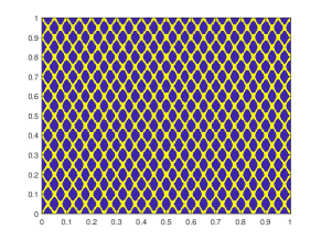
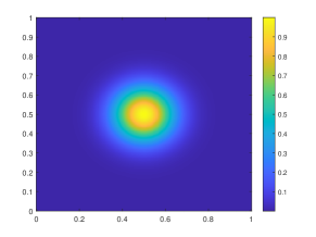
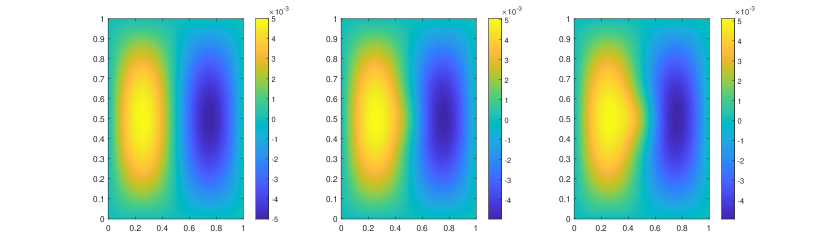
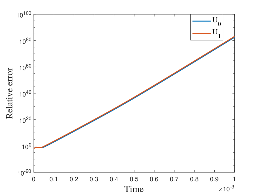
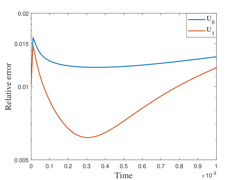
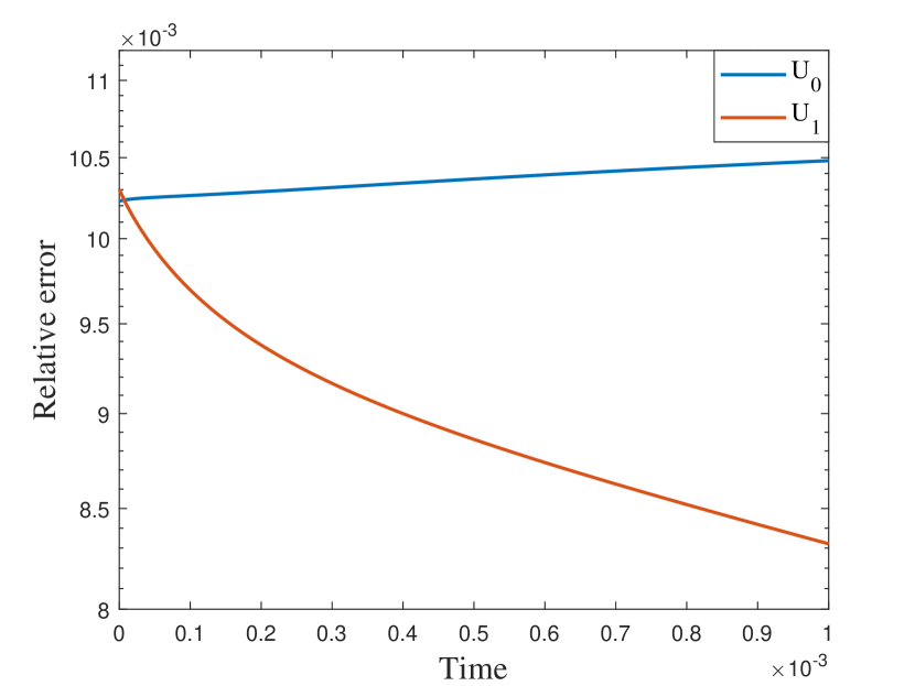
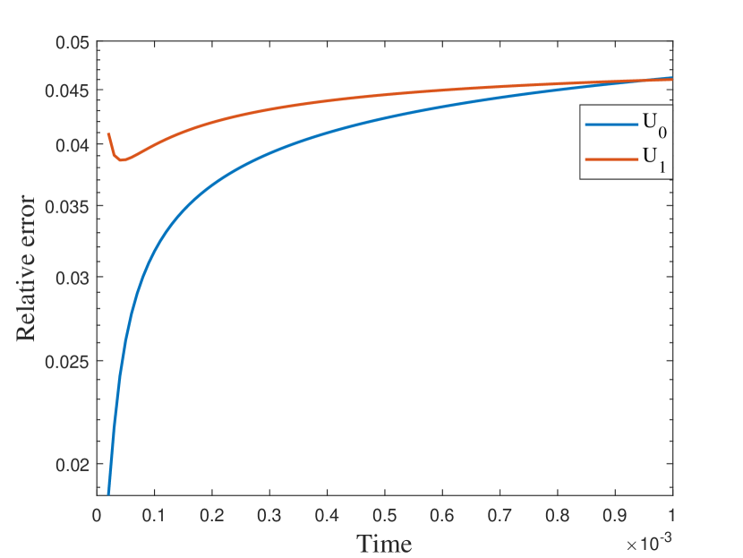
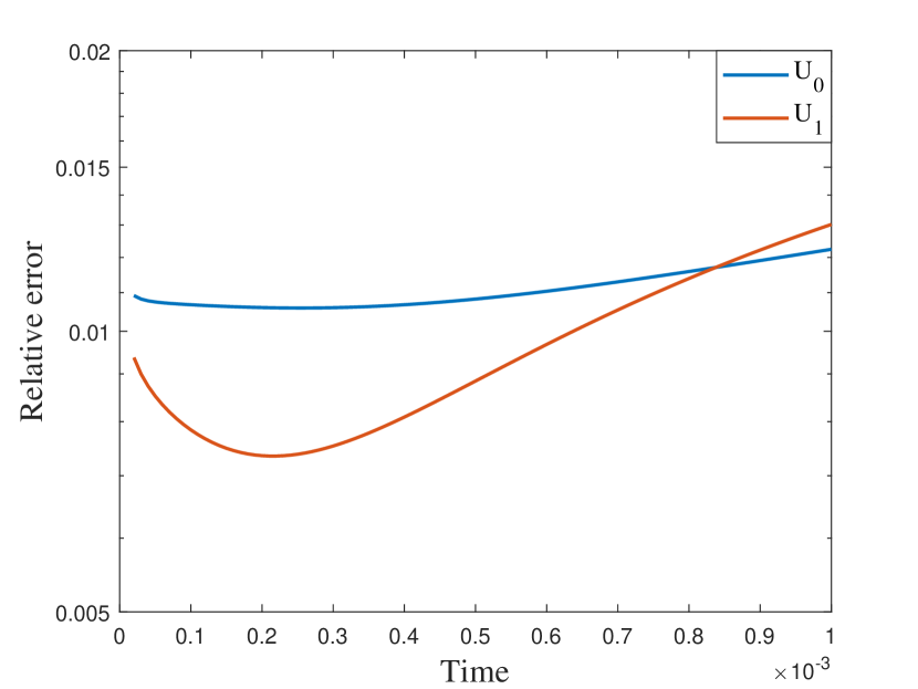
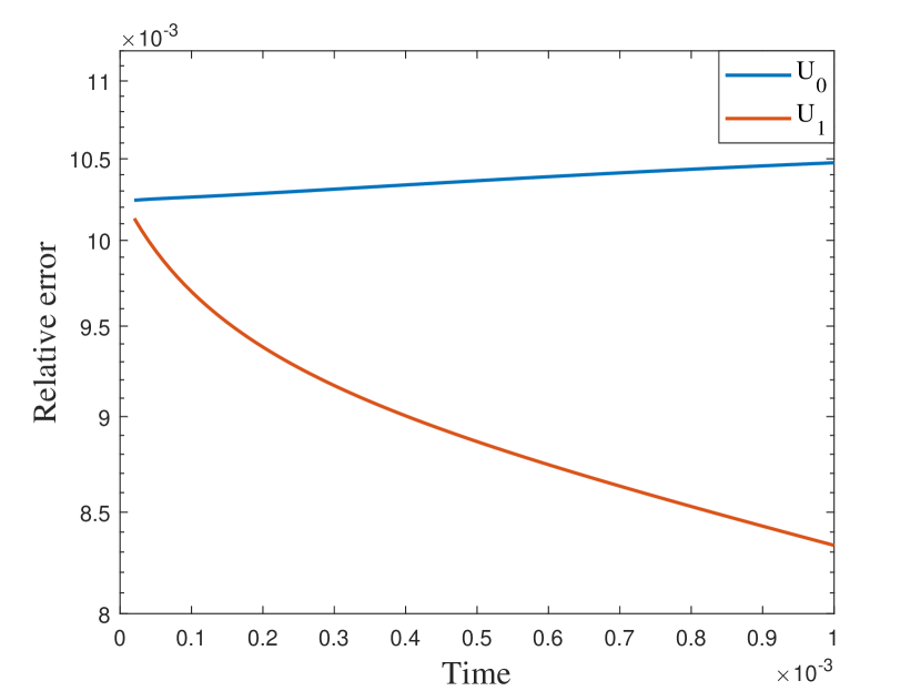
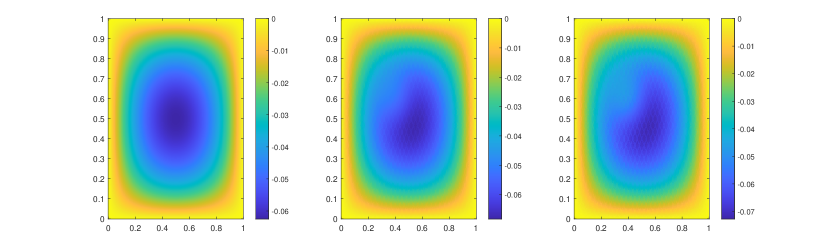
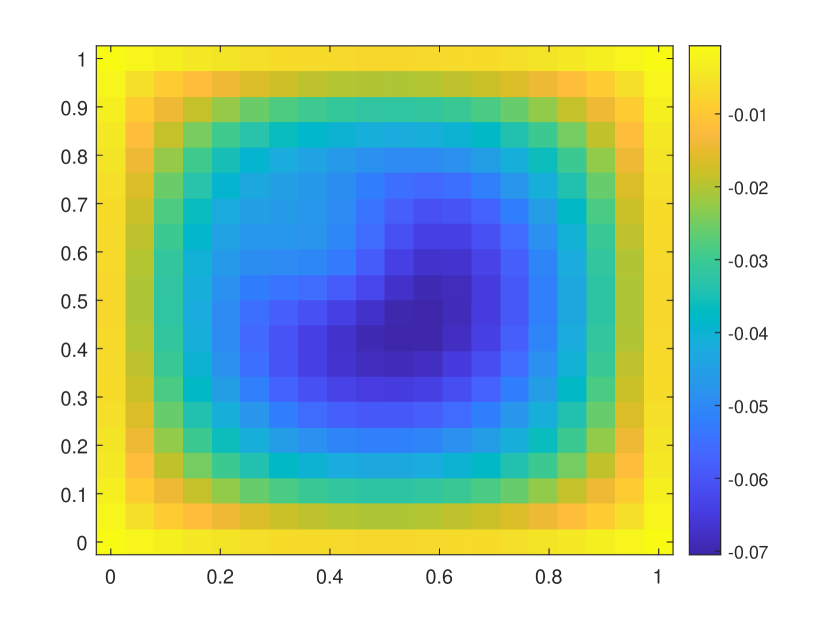
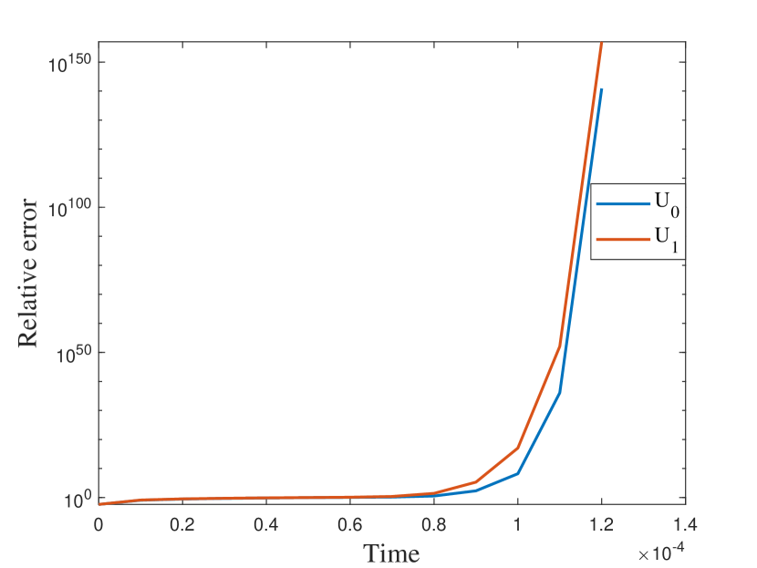
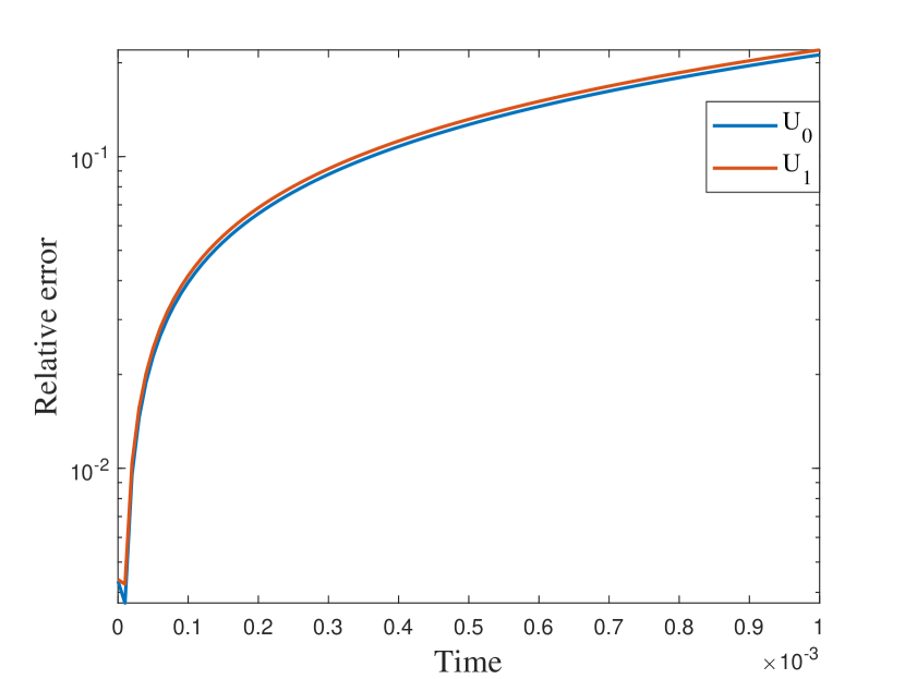
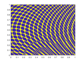
We first take a smooth source term $f(x_{1},x_{2})=\exp\bigl{(}\,-50((x_{1}-0.5)^{2}+(x_{2}-0.5)^{2})\,\bigr{)}$ and the initial condition $u_{0}(x_{1},x_{2})=5\times 10^{-3}\sin(2\pi x_{1})\sin(\pi x_{2})$ . In this example, we set $\alpha=0.9,0.6,0.3$ and $\varepsilon=\frac{1}{10}$ . The permeability field $\kappa$ is depicted in the left of Figure 2, which is a periodic field. The blue region represent the low conductivity region $\Omega_{0}$ while the yellow region represent the high conductivity region $\Omega_{1}$ . We plot the reference solution snapshots at $t=0,\ t=\frac{T}{2},\ t=T$ respectively in Figure 3. In Figure 4, we show the upscaled solutions and the corresponding averaged reference solutions for $\alpha=0.9$ at the final time. We note that our proposed approach provides an accurate approximation of the averaged reference solution for different $\alpha$ . Figure 5 shows the error history in the temporal direction corresponding to different $\alpha$ . Using same time step size, we compare the approximate solution obtained using explicit L1 and our proposed method. The relative errors at $t=T$ are shown in Table 1. It can be seen that for both methods, the approximation performs better when $\alpha$ is closer to $1$ . However, we observe that the explicit L1 scheme does not converge to the reference solutions when $\alpha$ goes to $0$ , while our method still gives good results, which demonstrates the effectiveness and stability of our proposed method.

$\alpha$	$U_{0}$		$U_{1}$
$\alpha$	Explicit L1	EI method	Explicit L1	EI method
0.9	0.0105	0.0105	0.0083	0.0083
0.6	0.0133	0.0122	0.0115	0.0130
0.3	NaN	0.0462	NaN	0.0460

Table 1: Relative errors at

t=T

5.2 Semilinear problems

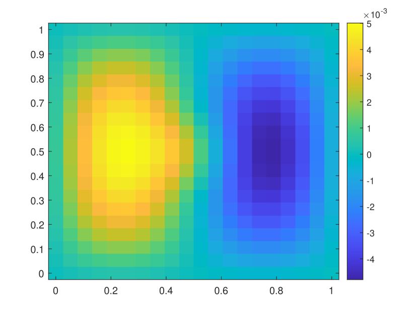
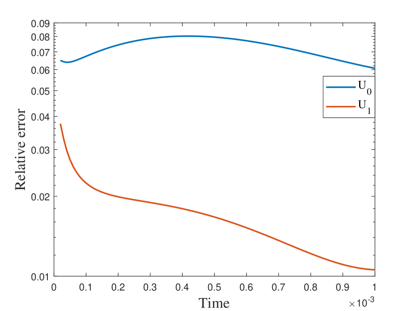
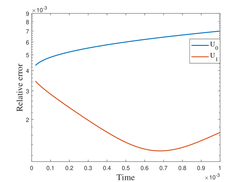
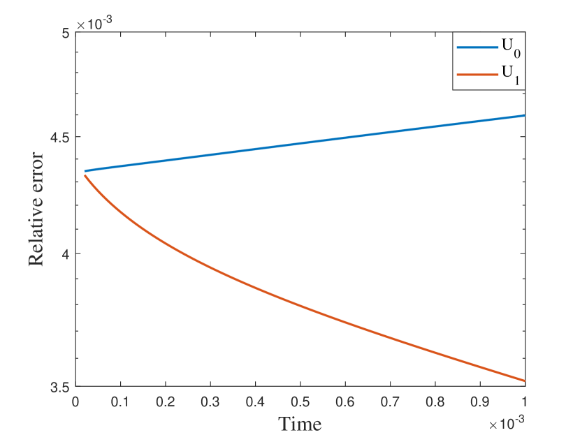
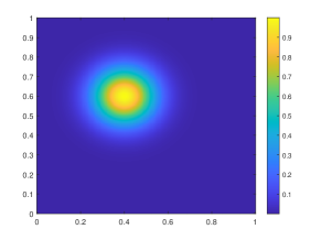
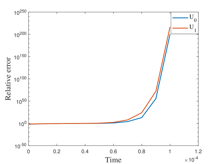
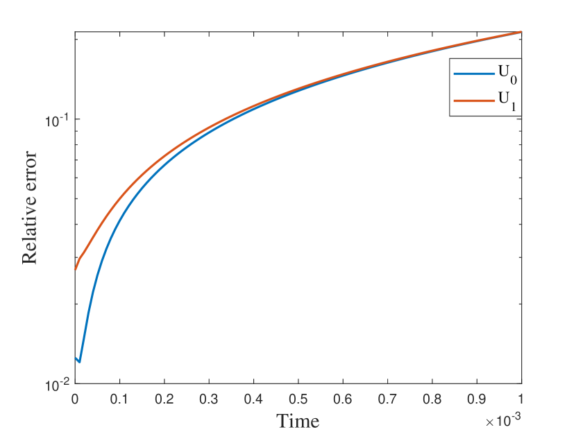
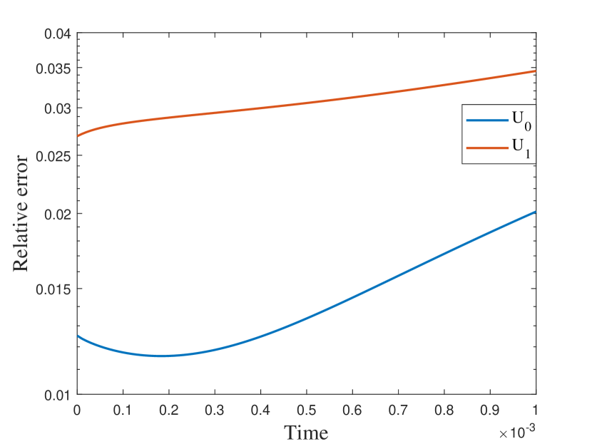
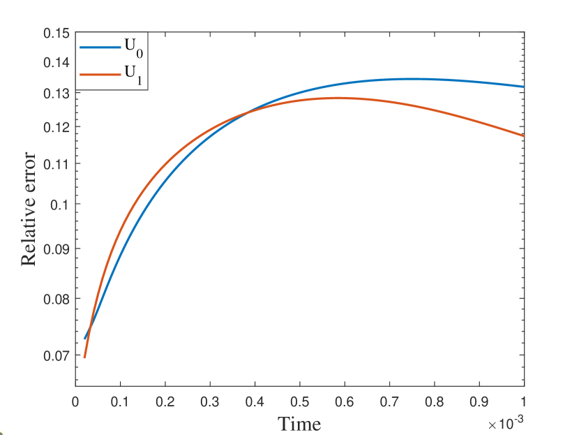
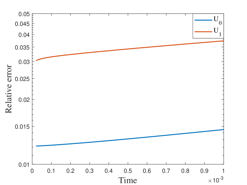
In this numerical test, we consider the semilinear problems and use the same media as in the first experiment. The results of the semilinear problems are also computed with different $\alpha$ by our proposed method. We take $f=u-u^{3}+f_{0}(x_{1},x_{2})$ with the initial condition $u_{0}(x_{1},x_{2})=-x_{1}(1-x_{1})x_{2}(1-x_{2})$ , where $f_{0}(x_{1},x_{2})=\exp\bigl{(}\,-50\bigl{(}\,(x_{1}-0.4)^{2}+(x_{2}-0.6)^{2}\,\bigr{)}\,\bigr{)}$ is the smooth source term shown in the right of Figure 9. We present the relative errors for different $\alpha=0.9,0.6,0.3$ . When $\alpha$ tends to $0$ , the explicit L1 scheme turns to be unstable while the EI method performs well. Moreover, for the semilinear problems, the L1 scheme needs iterative methods at each time step while the exponential integrator method does not. The reference solution snapshots are depicted in Figure 6. The Figure 7 illustrates the numerical solutions by L1 scheme and exponential integrator method compared to the average of the reference solutions. We figure out that our proposed method also works well for semilinear diffusion problems. We represent the relative errors in Figure 8 and Table 2 with different $\alpha$ .

$\alpha$	$U_{0}$		$U_{1}$
$\alpha$	Explicit L1	EI method	Explicit L1	EI method
0.9	0.0165	0.0046	0.0035	0.0176
0.6	0.2125	0.0070	0.2203	0.0019
0.3	NaN	0.0607	NaN	0.0106

Table 2: Relative errors at

t=T

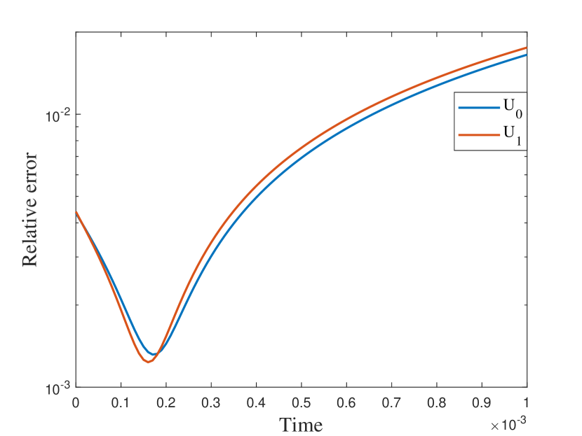
5.3 A more complicated media

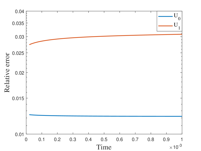
In our final example, we take nonperiodic media $\kappa$ as shown in the left of Figure 9. The other settings are the same as the previous semilinear case. We also represent the reference solution snapshots in Figure 10 with $\alpha=0.6$ . By the relative errors in Figure 11 and Table 3, the similar findings has been observed as in the previous cases. The errors of the numerical solutions is slightly larger compared to the previous examples, but they still converge to the reference solution.

$\alpha$	$U_{0}$		$U_{1}$
$\alpha$	Explicit L1	EI method	Explicit L1	EI method
0.9	0.0201	0.0122	0.0345	0.0308
0.6	0.2133	0.0145	0.2137	0.0374
0.3	NaN	0.1318	NaN	0.1173

Table 3: Relative errors at

t=T

6 Conclusions

In this paper, we present a time fractional multicontinuum upscaled model for solving the high-contrast fractional diffusion equation. The multicontinuum homogenization method is used to derive a coarse scale model, where the solutions are approximated through averages and accounts for gradient effects within each continuum, while incorporating microscale information in the upscaled quantities. We conduct a semi-discretized error analysis. We demonstrate that the nonlocal multicontinuum downscaling (NLMC) operator can be effectively approximated by the CEM-GMsFEM downscaling operator. Additionally, we utilize an exponential integrator approach for the time fractional derivative term and prove the convergence of the full discrete scheme. Numerical examples show that our method exhibits greater stability compared to the L1 scheme, while maintaining a similar convergence order. We explore various high-contrast heterogeneous media and source terms in our numerical experiments. It is noted that our proposed approach can be extended to scenarios involving two continua under appropriate assumptions. Future research would consist of addressing the singularity of the time fractional derivative and extended current approach to the high-order exponential integrator.

Acknowledgments

Y. Wang’s work is partially supported by the NSFC grant 12301559. W.T. Leung is partially supported by the Hong Kong RGC Early Career Scheme 21307223.

References

[1] Yalchin Efendiev and Thomas Y Hou. Multiscale finite element methods: theory and applications, volume 4. Springer Science & Business Media, 2009.
[2] Thomas Y Hou and Xiao-Hui Wu. A multiscale finite element method for elliptic problems in composite materials and porous media. Journal of computational physics, 134(1):169–189, 1997.
[3] Thomas Hou, Xiao-Hui Wu, and Zhiqiang Cai. Convergence of a multiscale finite element method for elliptic problems with rapidly oscillating coefficients. Mathematics of computation, 68(227):913–943, 1999.
[4] Zhiming Chen and Thomas Hou. A mixed multiscale finite element method for elliptic problems with oscillating coefficients. Mathematics of Computation, 72(242):541–576, 2003.
[5] Jennifer Dixon. On the order of the error in discretization methods for weakly singular second kind non-smooth solutions. BIT Numerical Mathematics, 25:623–634, 1985.
[6] Ch Lubich. Runge-kutta theory for volterra integrodifferential equations. Numerische Mathematik, 40:119–135, 1982.
[7] Alain Bourgeat. Homogenized behavior of two-phase flows in naturally fractured reservoirs with uniform fractures distribution. Computer Methods in Applied Mechanics and Engineering, 47(1-2):205–216, 1984.
[8] Louis J Durlofsky. Numerical calculation of equivalent grid block permeability tensors for heterogeneous porous media. Water resources research, 27(5):699–708, 1991.
[9] Yuguang Chen, Louis J Durlofsky, M Gerritsen, and Xian-Huan Wen. A coupled local–global upscaling approach for simulating flow in highly heterogeneous formations. Advances in water resources, 26(10):1041–1060, 2003.
[10] Xiao-Hui Wu, Yalchin Efendiev, and Thomas Y Hou. Analysis of upscaling absolute permeability. Discrete and Continuous Dynamical Systems Series B, 2(2):185–204, 2002.
[11] Yalchin Efendiev, Juan Galvis, and Thomas Y Hou. Generalized multiscale finite element methods (gmsfem). Journal of computational physics, 251:116–135, 2013.
[12] Yalchin Efendiev, Juan Galvis, and Xiao-Hui Wu. Multiscale finite element methods for high-contrast problems using local spectral basis functions. Journal of Computational Physics, 230(4):937–955, 2011.
[13] Eric T Chung, Yalchin Efendiev, and Wing Tat Leung. Residual-driven online generalized multiscale finite element methods. Journal of Computational Physics, 302:176–190, 2015.
[14] Axel Målqvist and Daniel Peterseim. Localization of elliptic multiscale problems. Mathematics of Computation, 83(290):2583–2603, 2014.
[15] Eric T Chung, Yalchin Efendiev, and Wing Tat Leung. Constraint energy minimizing generalized multiscale finite element method. Computer Methods in Applied Mechanics and Engineering, 339:298–319, 2018.
[16] Eric T Chung, Yalchin Efendiev, Wing Tat Leung, Maria Vasilyeva, and Yating Wang. Non-local multi-continua upscaling for flows in heterogeneous fractured media. Journal of Computational Physics, 372:22–34, 2018.
[17] Yalchin Efendiev and Wing Tat Leung. Multicontinuum homogenization and its relation to nonlocal multicontinuum theories. Journal of Computational Physics, 474:111761, 2023.
[18] Wing Tat Leung. Some convergence analysis for multicontinuum homogenization. arXiv preprint arXiv:2401.12799, 2024.
[19] Luis F Contreras, David Pardo, Eduardo Abreu, Judit Muñoz-Matute, Ciro Díaz, and Juan Galvis. An exponential integration generalized multiscale finite element method for parabolic problems. Journal of Computational Physics, 479:112014, 2023.
[20] Bangti Jin, Raytcho Lazarov, and Zhi Zhou. Numerical methods for time-fractional evolution equations with nonsmooth data: a concise overview. Computer Methods in Applied Mechanics and Engineering, 346:332–358, 2019.
[21] Guanglian Li. Wavelet-based edge multiscale parareal algorithm for subdiffusion equations with heterogeneous coefficients in a large time domain. Journal of Computational and Applied Mathematics, 440:115608, 2024.
[22] Yumin Lin and Chuanju Xu. Finite difference/spectral approximations for the time-fractional diffusion equation. Journal of computational physics, 225(2):1533–1552, 2007.
[23] Mengnan Li, Eric Chung, and Lijian Jiang. A constraint energy minimizing generalized multiscale finite element method for parabolic equations. Multiscale Modeling & Simulation, 17(3):996–1018, 2019.
[24] Igor Podlubny. Fractional differential equations: an introduction to fractional derivatives, fractional differential equations, to methods of their solution and some of their applications. elsevier, 1998.
[25] Zhengya Yang, Xuejuan Chen, Yanping Chen, and Jing Wang. Accurate numerical simulations for fractional diffusion equations using spectral deferred correction methods. Computers & Mathematics with Applications, 153:123–129, 2024.
[26] Steven M Cox and Paul C Matthews. Exponential time differencing for stiff systems. Journal of Computational Physics, 176(2):430–455, 2002.
[27] Roberto Garrappa and Marina Popolizio. Generalized exponential time differencing methods for fractional order problems. Computers & Mathematics with Applications, 62(3):876–890, 2011.
[28] Roberto Garrappa. Exponential integrators for time–fractional partial differential equations. The European Physical Journal Special Topics, 222(8):1915–1927, 2013.
[29] S Mohammed Hosseini and Zohreh Asgari. Solution of stochastic nonlinear time fractional pdes using polynomial chaos expansion combined with an exponential integrator. Computers & Mathematics with Applications, 73(6):997–1007, 2017.