An impossibility result for Markov Chain Monte Carlo sampling
from micro-canonical bipartite graph ensembles

Testing the statistical significance of properties of an observed network is a fundamental problem in network science [1]. The significance of the observed value is tested against a null model, an ensemble $\mathcal{H}=(\mathcal{G},{\color[rgb]{0,0,0}\pi})$ composed of the set $\mathcal{G}$ of possible graphs that can be realized under the null hypothesis and a probability distribution ${\color[rgb]{0,0,0}\pi}$ over $\mathcal{G}$. One typically selects some descriptive characteristics of the observed network, and either defines $\mathcal{G}$ and ${\color[rgb]{0,0,0}\pi}$ in such a way that the expectations w.r.t. ${\color[rgb]{0,0,0}\pi}$ of these characteristics over $\mathcal{G}$ are the same as the observed ones (a.k.a. the canonical model), or defines $\mathcal{G}$ as the set of all and only the graphs with exactly the same values for the characteristics as the observed network, and ${\color[rgb]{0,0,0}\pi}$ can be any distribution, often the uniform. Once the null model is defined, one proceeds by sampling several graphs from this ensemble. These graphs are used to approximate the distribution of the test statistic of interest under the null hypothesis. By comparing the observed statistic to this distribution one can compute an empirical $p$-value.

For example, the widely used “configuration model” [2] considers the set of graphs with the same degree sequence as the observed network and the uniform distribution. This model has been instrumental in determining that clustering, assortativity, and community structure in real networks are not solely dependent on node degrees, hence highlighting their significance [3]. However, the configuration model fails to generate graphs with a local structure similar to the observed graph [4]. Researchers have thus explored alternative null models that sample from graph families defined by more complex characteristics of the observed graph, such as joint degree distribution  [5, 4, 6, 7], core-value sequence [8], and local triangle-count sequence [9].

In this work, we focus on bipartite graphs, i.e., networks whose nodes can be partitioned into two classes such that all edges go from one class to the other. Formally, a bipartite graph is a tuple $G\doteq(L,R,E)$, where $L$ and $R$ are disjoint sets of nodes called left and right nodes, respectively, and $E\subseteq L\times R$ is a set of edges connecting nodes in $L$ to nodes in $R$. We consider undirected bipartite graphs, but for ease of presentation, we denote any edge $(u,a)$ so that $u\in L$ and $a\in R$. For any vertex $v\in L\cup R$ we denote with $\Gamma_{G}\lparen v\rparen$ the set of neighbors of $v$, i.e., the vertices to which $v$ is connected by an edge in $G$, and we define the degree $\mathsf{d}_{G}\lparen v\rparen$ of $v$ in $G$ as $\mathsf{d}_{G}\lparen v\rparen\doteq\left\lvert\Gamma_{G}\lparen v\rparen\right\rvert$. Assuming an arbitrary but fixed labeling $u_{1},\dotsc,u_{\left\lvert L\right\rvert}$ (resp. $a_{1},\dotsc,a_{\left\lvert R\right\rvert}$) of the nodes in $L$ (resp. $R$), the vector $\langle\mathsf{d}_{G}\lparen u_{1}\rparen,\dotsc,\mathsf{d}_{G}\lparen u_{\left\lvert L\right\rvert}\rparen\rangle$ (resp. $\langle\mathsf{d}_{G}\lparen a_{1}\rparen,\dotsc,\mathsf{d}_{G}\lparen a_{\left\lvert R\right\rvert}\rparen\rangle$) is known as the left (resp. right) degree sequence of $G$.

Bipartite networks occur naturally in many applications: when representing words and documents [10], items and itemsets [11], higher-order networks such as hypergraphs and simplicial complexes [12], and many more. Null models and graph ensembles can also be defined on bipartite graphs [13, 11, 14]. For example, Preti et al. [11] introduce a null model that preserves the bipartite joint adjacency matrix (i.e., the matrix whose $(i,j)$-th entry is the number of edges connecting nodes from $L$ with degree $i$ to nodes in $R$ with degree $j$), of an observed network (thus the degree sequences and the number of caterpillars, i.e., paths of length 3), and give Markov Chain Monte Carlo (MCMC) algorithms to sample from this null model. Null models for bipartite graphs are also of particular interest because they align with null models for 0–1 binary matrices [15, Ch. 6]. For example, preserving the degree sequences in a bipartite graph corresponds to preserving the row and column marginals of the corresponding bi-adjacency matrix, and several MCMC algorithms have been developed to sample from this null model [16, 17, 18, 19, 20].

We consider graph ensembles for which $\mathcal{G}$ is the set of all bipartite graphs $G\doteq(L,R,E)$ that share the same degree sequences and the same number of butterflies, i.e., $k_{2,2}$ bi-cliques , defined as follows.

The following result, whose proof is immediate, gives an expression for the number of butterflies to which two nodes both belong.

For $u\in L$, we denote with $\mathsf{b}_{G}\lparen u\rparen$ the number of butterflies in $G$ to which $u$ belongs. It holds

The total number $\mathsf{b}\lparen G\rparen$ of butterflies in $G$ is then

The butterfly, being the smallest complete subgraph in a bipartite graph, is the most basic building block for composing more complex structures, analogous to the triangle in unipartite graphs. Consequently, preserving the number of butterflies emerges as a natural choice when defining null models that retain more graph properties beyond just the degree sequences. This concept finds applications in studying, e.g., clustering patterns [21].

MCMC methods are a popular approach to sample from an ensemble $\mathcal{H}=(\mathcal{G},{\color[rgb]{0,0,0}\pi})$. They define a suitable Markov chain on the space $\mathcal{G}$ of all possible graphs, such that, after a sufficient burn-in period, the state of the Markov chain is approximately distributed according to ${\color[rgb]{0,0,0}\pi}$. The correctness of this process requires the Markov chain to be finite, irreducible, and aperiodic [2]. Efficient sampling requires not only that the Markov chain has a fast mixing time, but also that the space can be explored quickly, i.e., that obtaining a neighbor from the current state is efficient. The double edge swap technique, also known as degree-preserving rewiring [22], checkerboard swap [23], or tetrad [17], is a simple yet fundamental randomization technique used to generate a new graph with the same degree sequence as a given graph. Its efficiency stems from the fact that it involves the rewiring of a small number of edges. In bipartite graphs, the most basic rewiring technique is known as the bipartite swap operation (BSO).

A more sophisticated operation is the $q$-edge bipartite swap operation ($q$-BSO), which may involve the simultaneous swapping of multiple edges, potentially between a large set of nodes, similar to the $q$-switch operation defined by Tabourier et al. [24].

According to this definition, a BSO involving $(u,a)$ and $(v,b)$ can be seen as the $2$-BSO $(\langle(u,a),(v,b)\rangle,(2\ 1))$. Algorithms such as Verhelst’s [17] and Curveball [20] aim to speed up the sampling from the ensemble of bipartite graphs with fixed degree sequences. They execute multiple BSO operations at each step by selecting nodes $u$ and $v$ from $L$ (or $R$) and exchanging multiple edges originating from $u$ with edges originating from $v$. Conversely, a $q$-BSO may involve the simultaneous swapping of multiple edges originating from multiple source nodes. Thus, the moves considered by Curveball and Verhelst’s can be expressed as $q$-BSOs, but $q$-BSOs are more expressive, in the sense that there are $q$-BSOs that do not correspond to possible moves for these algorithms.

A key requirement to use an MCMC method for sampling from a graph ensemble is that the state space, where each state corresponds to a graph in the ensemble, is strongly connected , i.e., for any two states $G^{\prime}$ and $G^{\prime\prime}$ there is a sequence $\langle\rho_{1},\rho_{2},\dotsc,\rho_{\ell}\rangle$ of graph-transforming operations for some $\ell$ (which may depend on the chosen $G^{\prime}$ and $G^{\prime\prime})$, such that $\rho_{1}$ transforms $G^{\prime}$ into some $G_{1}$ that belongs to the state space, $\rho_{i}$ for $1<i<\ell$ transforms $G_{i}$ into $G_{i+1}$ that also belongs to the state space, and $\rho_{\ell}$ transforms $G_{\ell-1}$ into $G^{\prime\prime}$. In other words, a class $\mathcal{C}$ of graph-transforming operations defines a neighborhood structure of the state space as follows: given any $G$ in the state space, a neighbor of $G$ is any state that can be obtained by applying a single operation from $\mathcal{C}$, provided that the operation is applicable to $G$. With this neighborhood structure, the state space is strongly connected if there is a path from any state to any other state.

We can immediately see that the state space $\mathcal{G}$ we consider is strongly connected by sequences of $q$-BSOs when $q$ is large enough, for any left and right degree sequences, and any number of butterflies (see also [24, Sect. 3.2.2]). In fact, there is always a $\left\lvert E^{\prime}\setminus E^{\prime\prime}\right\rvert$-BSO that transforms any bipartite graph $G^{\prime}\doteq(L,R,E^{\prime})$ into another bipartite graph $G^{\prime\prime}\doteq(L,R,E^{\prime\prime})$ with the same left and right degree sequences, and number of butterflies (see Supplementary Material [25] for details). While this fact ensures the strong connectivity of the state space via the union of all $q$-BSOs for $q=2,\dotsc,\left\lvert E^{\prime}\right\rvert$, it has little practical relevance, as we now explain. If we use all these $q$-BSOs to define the neighborhood structure of the state space, the resulting space would be a complete graph, i.e., a clique. Consequently, drawing, according to any distribution, a neighbor of a given state would require a procedure to build an entirely new bipartite graph with the same degree sequences and the same number of butterflies from scratch. Developing such a procedure seems even harder than the problem we are attempting to solve, in the same way as devising algorithms for building a bipartite graph with prescribed degree sequences from scratch [26, 27, 28, 29, 30] is much harder than devising algorithms for sampling such a graph using MCMC approaches starting from an existing one [17, 20, 16, 18, 19].

The correct question to ask is therefore the following: is there a fixed, universal, constant $q^{*}$ such that, for any left and right degree sequences, and any number of butterflies, any two bipartite graphs with those left and right degree sequences, and that number of butterflies, are connected by sequences $\langle\mathsf{sw}^{p_{1}}_{1}=(S_{1},\sigma_{1}),\dotsc,\mathsf{sw}^{p_{z}}_{z}=(S_{z},\sigma_{z})\rangle$ of $p_{i}$-BSOs, with $p_{i}\leq q^{*}$, $i=1,\dotsc,z$, where $z$ may depend on the two graphs? By “universal”, we mean a quantity that in no way depends on properties of the ensemble $(\mathcal{G},\pi)$, including properties of the observed network.

Asking this question is reasonable: it is known that $q^{*}=2$ when one is only interested in preserving the degree sequences [15, Ch. 6], and it is also known that $q^{*}=2$ for the case of preserving the degree sequences and the number of paths of length 3 (a.k.a. caterpillars), in which case the rewiring operations slightly differ from the traditional BSOs [11, 31].

Additionally, we would like $q^{*}$ to be small, because sampling a $q$-BSO is not necessarily efficient: the naïve approach of independently sampling $q$ edges and then verifying whether they form a valid $q$-BSO has an increasing probability of failure as $q$ increases [24]. As a result, the Markov chain would exhibit a high probability of staying in the same state for many consecutive steps, greatly increasing the mixing time.

For unipartite graphs, it has been proved that $q^{*}=2$ is not always sufficient to ensure strong connectivity of spaces of graphs that share more complex properties [24, 31]. In this work, we demonstrate the nonexistence of a fixed, universal, constant $q^{*}$ for the ensemble of bipartite graphs with the same left and right degree sequences and the same number of butterflies.

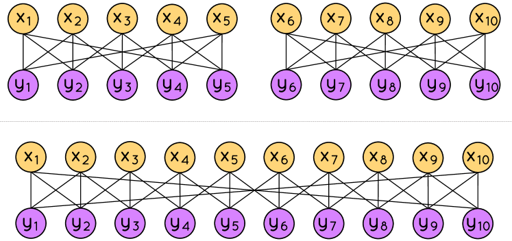
Let us give some intuition with an example, which shows that it cannot be $q^{*}<4$. Figure 1 shows two bipartite graphs $G_{1}$ (upper) and $G_{2}$ (lower) with the same left and right degree sequences, and the same number of butterflies $\mathsf{b}\lparen G_{1}\rparen=\mathsf{b}\lparen G_{2}\rparen=10$. There is no sequence of $q$-BSO s for $q<4$ that, when applied to $G_{1}$, generates a graph isomorphic to $G_{2}$: any $q$-BSO for $q<4$ applied to $G_{1}$ either generates a graph with a different number of butterflies, or generates a graph isomorphic to $G_{1}$. On the other hand, the $4$-BSO $([(x_{1},y_{5}),(x_{5},y_{1}),(x_{6},y_{10}),(x_{10},y_{6})],\sigma)$ with $\sigma(1)=3$, $\sigma(2)=4$, $\sigma(3)=1$, and $\sigma(4)=2$ ensures that the two butterflies $\{x_{1},x_{5},y_{1},y_{5}\}$ and $\{x_{6},x_{10},y_{6},y_{10}\}$ disappear, while the two new butterflies $\{x_{1},x_{10},y_{1},y_{10}\}$ and $\{x_{5},x_{6},y_{5},y_{6}\}$ appear, hence preserving the total count $\mathsf{b}\lparen G_{1}\rparen$.

Our main result is the following theorem (proof in Supplementary Material [25]).

Our proof consists of two parts. First, we construct two bipartite graphs $G_{\mathrm{b}}$ and $G_{\mathrm{e}}$ with the same left and right degree sequences (which will depend on $\bar{q}$ as the second largest left degree will be greater than $\bar{q}$), and the same number of butterflies. Second, we demonstrate that any sequence of $q$-BSOs applied to $G_{\mathrm{b}}$ to obtain a graph isomorphic to $G_{\mathrm{e}}$ must involve at least one $q$-BSO for $q>\bar{q}$. Since $\bar{q}$ can be arbitrarily large, a universal constant $q^{*}$ as above cannot exist.

This theorem proves that it is impossible to design efficient MCMC algorithms that sample from ensembles $\mathcal{H}=(\mathcal{G},{\color[rgb]{0,0,0}\pi})$ of bipartite graphs with the same degree sequences and the same number of butterflies, because the state space is not strongly connected by edge swap operations that involve only up to a fixed, universal, number of edges, as is instead the case for simpler null models. Rather, the minimum number of edges that must be involved depends on properties of the state space $\mathcal{G}$ , not just of the observed network. These may not be easily computable, as they may not depend just on the observed network, if any.

This result has profound implications for the design of network null models and for network science in general. If it is unfeasible to preserve the occurrences of the simplest building block of bipartite graphs (the butterfly), it becomes unfeasible to preserve larger structures. When dealing with bipartite graphs and complex observed characteristics, ensembles with “soft” constraints, where the constraints are retained on average over all the graphs sampled from the ensemble [32], might be the only viable option.

The algorithm to construct the graphs $G_{\mathrm{b}}$ and $G_{\mathrm{e}}$ is delineated in the Supplementary Material [25]. We now describe the main characteristics of such graphs.

Let $s$ and $t$ be two naturals with $s>t\geq 2$ and $2(s-1)>\bar{q}$. We define $n\doteq\binom{s}{2}+\binom{t}{2}$ and $a\doteq((s+1)\ \text{mod}\ 2)+((t+1)\ \text{mod}\ 2)$. The graphs $G_{\mathrm{b}}$ and $G_{\mathrm{e}}$ output by the algorithm with inputs $s$ and $t$ have the following properties:

1. 1.

   $G_{\mathrm{b}}$ and $G_{\mathrm{e}}$ have $7+a$ left nodes (denoted with the letter $x$) and $s+t+n+2+a$ right nodes (denoted with the letter $y$);

2. 2.

   $G_{\mathrm{b}}$ and $G_{\mathrm{e}}$ have the same left and right degree sequences. In particular, $x_{1}$ and $x_{2}$ have degree $s$, $x_{3}$ and $x_{4}$ have degree $t$, $x_{5}$ and $x_{6}$ have degree $n+1$, $y_{i}$ has degree 2 for $1\leq i\leq s+t+n+1$, and all the other left and right nodes have degree $1$;

3. 3.

   $\mathsf{b}\lparen G_{\mathrm{b}}\rparen=\mathsf{b}\lparen G_{\mathrm{e}}\rparen=n+\binom{n}{2}$;

4. 4.

   $\left\lvert\Gamma_{G_{\mathrm{e}}}\lparen x_{5}\rparen\cap\Gamma_{G_{\mathrm{e}}}\lparen x_{6}\rparen\right\rvert=n+1$, which, with the previous point, implies that $x_{5}$ and $x_{6}$ belong to all butterflies in $G_{\mathrm{e}}$, and every other node $y\in R$ belongs to no butterfly;

5. 5.

   $\left\lvert\Gamma_{G_{\mathrm{b}}}\lparen x_{5}\rparen\cap\Gamma_{G_{\mathrm{b}}}\lparen x_{6}\rparen\right\rvert=n$, $\left\lvert\Gamma_{G_{\mathrm{b}}}\lparen x_{1}\rparen\cap\Gamma_{G_{\mathrm{b}}}\lparen x_{2}\rparen\right\rvert=s$, $\left\lvert\Gamma_{G_{\mathrm{b}}}\lparen x_{3}\rparen\cap\Gamma_{G_{\mathrm{b}}}\lparen x_{4}\rparen\right\rvert=t$, which implies, with point 2, that $x_{5}$ and $x_{6}$ do not belong to all butterflies in $G_{\mathrm{b}}$.

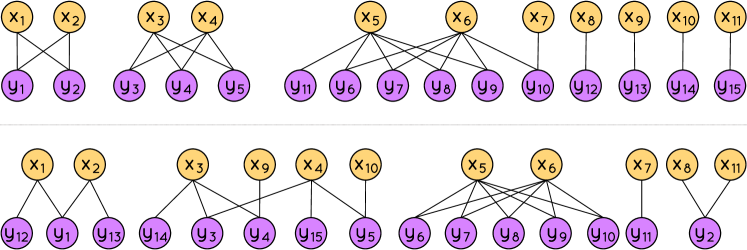
Figure 2 shows the bipartite graphs generated for $s=2$ and $t=3$.

MCMC approaches based on swaps of pairs of edges can efficiently sample graphs from simple ensembles, such as those including graphs with prescribed degree sequences, or fixed number of paths of length up to three [11]. The correctness of these approaches relies on the fact that pairwise edge swaps create a strongly connected state space. They are efficient because proposing a neighbor to move to is relatively easy, requiring only to be able to efficiently sample pairs of edges.

In the case of ensembles preserving more complex properties of the networks, the strong connectivity of the state space may require more than two edges to be swapped at every step, i.e., performing $q$-switches [24], or $q$-BSOs, for some value of $q$.

In this work, we consider the ensemble of bipartite graphs with fixed degree sequences and fixed number of butterflies ($k_{2,2}$ bi-cliques), for its important role in a variety of applications, e.g., investigating clustering patterns [21]. We show that the state space is not strongly connected by sequences of $q$-BSOs for any fixed, universal, constant $q$. In other words, the number of edges to be rewired at each step is upper bounded by a quantity that depends on properties of the graphs in the ensemble. This result is in strong contrast with the cases for the space of bipartite graphs with fixed degree sequences, and for that of bipartite graphs with fixed degree sequences and fixed number of paths of length three (a.k.a. caterpillars), where $q=2$ is sufficient for all ensembles [11, 31].

This discovery has far-reaching implications for network science. First and foremost, we rule out the possibility of designing efficient MCMC algorithms for sampling from the space of bipartite graphs with fixed degree sequences and fixed number of butterflies, specifically, from the micro-canonical ensemble that maintains these properties exactly. In fact, we demonstrate the necessity of swaps with size dependent on the characteristics of the graph space $\mathcal{G}$, not necessarily just on the observed network. Finding what this size $q^{*}_{\mathcal{G}}$ is may not even be feasible. It may perhaps be possible to develop an efficient procedure to find this quantity, but then one also needs an efficient procedure to, at each step of the Markov chain, generate a $q$-BSO for $q\leq q^{*}_{\mathcal{G}}$, to propose a neighbor to move to. Solving both these algorithmic questions seem challenging. Moreover, the lower bound $\bar{q}$ to the size of the BSOs needed to connect the two graphs $G_{\mathrm{b}}$ and $G_{\mathrm{e}}$ from Thm. 1 gives only a necessary condition for the strong connectivity of the graph space, not a sufficient one: we only know that one of the BSOs to connect these two graphs must contain more than $\bar{q}$ edges, but not how exactly how many. Even if we knew exactly this number $\hat{q}$, there may be other pairs of graphs in the same ensemble (i.e., with the same degree sequences and number of butterflies) such that any sequence of BSOs connecting these two graphs must have size even greater than $\hat{q}$. Therefore the situation might be even more dire than our findings suggest.

Given that sampling from a null model that preserves the number of butterflies is impractical, preserving larger structures seems an even more unattainable task. A butterfly is at the same time the smallest cycle and the smallest non-trivial bi-clique, hence it is a basic building block of bipartite graphs. Thus, our findings present a large obstacle to developing efficient algorithms to sample from more complex ensembles, and therefore to testing network properties under more descriptive null models.

What other options are then available, if any? If one wishes to maintain the number of butterflies as a hard constraint (i.e., to sample from the micro-canonical ensemble), one potential approach involves avoiding MCMC algorithms and opting for a direct-sampling algorithm like stub matching [33]. However, such algorithms are already limited to small graph instances, for the case of sampling from the space of graphs with the same degree sequence, due to their complexity scaling quadratically or cubically with the number of nodes, depending on the graph density [34, 35]. The straightforward application of existing stub-matching techniques may also suffer from generating graphs with a different number of butterflies, thus leading to a high rejection rate. Thus, we need to explore alternative methodologies or refine existing stub-matching algorithms to better accommodate these more complex constraints. Finally, implementations of canonical methods such as the Chung-Lu model [36] offer a more efficient alternative, albeit at the cost of imposing a soft constraint. Indeed, while the ensemble average aligns precisely with the desired value of each constraint, individual graph instances may lie far from the desired constraints. The canonical ensemble brings other challenges, including difficulties in generating graphs that closely match the desired expectations for certain degree distributions (degeneracy problem) [37, 38, 39, 40, 41].

Overall, our findings represent a strong negative result that the network science community needs to reckon with. By showing that this research avenue is not fruitful, we hope to spur alternative and innovative approaches to designing null models for graphs, and algorithms for sampling from them.

References

- Newman [2003] M. E. Newman, SIAM review 45, 167 (2003).
- Fosdick et al. [2018] B. K. Fosdick, D. B. Larremore, J. Nishimura, and J. Ugander, Siam Review 60, 315 (2018).
- Cimini et al. [2019] G. Cimini, T. Squartini, F. Saracco, D. Garlaschelli, A. Gabrielli, and G. Caldarelli, Nature Reviews Physics 1, 58 (2019).
- Stanton and Pinar [2012] I. Stanton and A. Pinar, Journal of Experimental Algorithmics (JEA) 17, 3 (2012).
- Mahadevan et al. [2006] P. Mahadevan, D. Krioukov, K. Fall, and A. Vahdat, ACM SIGCOMM Computer Communication Review 36, 135 (2006).
- Orsini et al. [2015] C. Orsini, M. M. Dankulov, P. Colomer-de Simón, A. Jamakovic, P. Mahadevan, A. Vahdat, K. E. Bassler, Z. Toroczkai, M. Boguná, G. Caldarelli, et al., Nature communications 6, 8627 (2015).
- Bassler et al. [2015] K. E. Bassler, C. I. Del Genio, P. L. Erdős, I. Miklós, and Z. Toroczkai, New Journal of Physics 17, 083052 (2015).
- Van Koevering et al. [2021] K. Van Koevering, A. Benson, and J. Kleinberg, in The Web Conference 2021 (2021) pp. 367–378.
- Newman [2009] M. E. Newman, Physical review letters 103, 058701 (2009).
- Zha et al. [2001] H. Zha, X. He, C. Ding, H. Simon, and M. Gu, in CIKM (2001) pp. 25–32.
- Preti et al. [2022] G. Preti, G. de Francisci Morales, and M. Riondato, in ICDM (IEEE, 2022) pp. 418–427.
- Berge [1970] C. Berge, in Combinatorial Theory and its Applications I, Colloquia Mathematica Societatis János Bolyai, Vol. 4 (1970) pp. 119–133.
- Saracco et al. [2015] F. Saracco, R. Di Clemente, A. Gabrielli, and T. Squartini, Scientific reports 5, 1 (2015).
- Neal et al. [2023] Z. Neal, A. Cadieux, D. Garlaschelli, N. J. Gotelli, F. Saracco, T. Squartini, S. T. Shutters, W. Ulrich, G. Wang, and G. Strona (2023), arXiv 2310.01284.
- Ryser [1963] H. J. Ryser, Combinatorial mathematics, Vol. 14 (American Mathematical Soc., 1963).
- Carstens [2015] C. J. Carstens, Physical Review E 91, 042812 (2015).
- Verhelst [2008] N. D. Verhelst, Psychometrika 73, 705 (2008).
- Wang [2020] G. Wang, Electronic Journal of Statistics 14, 1690 (2020).
- Kannan et al. [1999] R. Kannan, P. Tetali, and S. Vempala, Random Structures & Algorithms 14, 293 (1999).
- Strona et al. [2014] G. Strona, D. Nappo, F. Boccacci, S. Fattorini, and J. San-Miguel-Ayanz, Nature communications 5, 1 (2014).
- Nishimura [2017] J. Nishimura, arXiv preprint arXiv:1704.01951 (2017).
- Cafieri et al. [2010] S. Cafieri, P. Hansen, and L. Liberti, Physical Review E 81, 046102 (2010).
- Artzy-Randrup and Stone [2005] Y. Artzy-Randrup and L. Stone, Physical Review E 72, 056708 (2005).
- Tabourier et al. [2011] L. Tabourier, C. Roth, and J.-P. Cointet, ACM Journal of Experimental Algorithmics 16, 7:1 (2011).
- [25] See Supplemental Material at URL-will-be-inserted-by-publisher for proofs and algorithmic details.
- Chen et al. [2005] Y. Chen, P. Diaconis, S. P. Holmes, and J. S. Liu, Journal of the American Statistical Association 100, 109 (2005).
- Miller and Harrison [2013] J. W. Miller and M. T. Harrison, The Annals of Statistics 41, 10.1214/13-aos1131 (2013).
- Holmes and Jones [1996] R. Holmes and L. Jones, The Annals of Statistics , 64 (1996).
- Miklós and Podani [2004] I. Miklós and J. Podani, Ecology 85, 86 (2004).
- Snijders [1991] T. A. Snijders, Psychometrika 56, 397 (1991).
- Czabarka et al. [2015] É. Czabarka, A. Dutle, P. L. Erdős, and I. Miklós, Discrete Applied Mathematics 181, 283 (2015).
- Robins et al. [2007] G. Robins, P. Pattison, Y. Kalish, and D. Lusher, Social networks 29, 173 (2007).
- Bollobás [1980] B. Bollobás, European Journal of Combinatorics 1, 311 (1980).
- Erdős et al. [2009] P. L. Erdős, I. Miklós, and Z. Toroczkai, arXiv preprint arXiv:0905.4913 (2009).
- Kim et al. [2012] H. Kim, C. I. Del Genio, K. E. Bassler, and Z. Toroczkai, New Journal of Physics 14, 023012 (2012).
- Chung and Lu [2002] F. Chung and L. Lu, Proceedings of the National Academy of Sciences 99, 15879 (2002).
- Squartini and Garlaschelli [2011] T. Squartini and D. Garlaschelli, New Journal of Physics 13, 083001 (2011).
- Squartini et al. [2015] T. Squartini, R. Mastrandrea, and D. Garlaschelli, New Journal of Physics 17, 023052 (2015).
- Brissette and Slota [2022] C. Brissette and G. Slota, in Proceedings of the Tenth International Conference on Complex Networks and Their Applications (Springer, 2022) pp. 451–462.
- Snijders et al. [2006] T. A. Snijders, P. E. Pattison, G. L. Robins, and M. S. Handcock, Sociological methodology 36, 99 (2006).
- Vallarano et al. [2021] N. Vallarano, M. Bruno, E. Marchese, G. Trapani, F. Saracco, G. Cimini, M. Zanon, and T. Squartini, Scientific Reports 11, 10.1038/s41598-021-93830-4 (2021).
Appendix A Proofs
Our main result, Theorem 1, relies on the following lemma.
Lemma 1.
For any bipartite graph with , for each , and any , it holds
with equality if and only if there exists , s.t. .
The meaning of this Lemma is that, when all nodes in have degree at most 2 , each node can be part of at most one butterfly for each unordered pair of ’s neighbors. Specifically, if either or has degree , then there can be no butterfly involving , , and another node in . If both and have degree , there may be at most one butterfly involving , , and another node in . If any node in has degree , a pair of neighbors of could be part of more than one butterfly together with (at most ).
We use the following technical lemma in the proof of Lemma 1.
Lemma 2.
Let , . For any sequence of strictly positive naturals s.t. , it holds
Proof.
Assume by contradiction that there exists a sequence of strictly positive naturals s.t. and for which