An Improved Square-root Algorithm for V-BLAST Based on Efficient Inverse Cholesky Factorization

Multiple-input multiple-output (MIMO) wireless communication systems can achieve huge channel capacities [1] in rich multi-path environments through exploiting the extra spatial dimension. Bell Labs Layered Space-Time architecture (BLAST) [2], including the relative simple vertical BLAST (V-BLAST) [3], is such a system that maximizes the data rate by transmitting independent data streams simultaneously from multiple antennas. V-BLAST often adopts the ordered successive interference cancellation (OSIC) detector [3], which detects the data streams iteratively with the optimal ordering. In each iteration, the data stream with the highest signal-to-noise ratio (SNR) among all undetected data streams is detected through a zero-forcing (ZF) or minimum mean-square error (MMSE) filter. Then the effect of the detected data stream is subtracted from the received signal vector.

Some fast algorithms have been proposed [4, 5, 6, 7, 10, 11, 8, 9] to reduce the computational complexity of the OSIC V-BLAST detector [3]. An efficient square-root algorithm was proposed in [4] and then improved in [5], which also partially inspired the modified decorrelating decision-feedback algorithm [6]. In additon, a fast recursive algorithm was proposed in [7] and then improved in [8, 9, 10, 11]. The improved recursive algorithm in [8] requires less multiplications and more additions than the original recursive algorithm [7]. In [9], the author gave the “fastest known algorithm” by incorporating improvements proposed in [10, 11] for different parts of the original recursive algorithm [7], and then proposed a further improvement for the “fastest known algorithm”.

On the other hand, most future cellular wireless standards are based on MIMO Orthogonal Frequency Division Multiplexing (OFDM) systems, where the OSIC V-BLAST detectors [3, 4, 5, 6, 7, 10, 11, 8, 9] require an excessive complexity to update the detection ordering and the nulling vectors for each subcarrier. Then simplified V-BLAST detectors with some performance degradation are proposed in [12, 13], which update the detection [12] or the detection ordering [13] per group of subcarriers to reduce the required complexity.

In this letter, a fast algorithm for inverse Cholesky factorization [14] is deduced to compute a triangular square-root of the estimation error covariance matrix for V-BLAST. Then it is employed to propose an improved square-root V-BLAST algorithm, which speedups several steps in the previous square-root V-BLAST algorithm [5], and can offer further computational savings in MIMO OFDM systems.

This letter is organized as follows. Section \@slowromancapii@ describes the V-BLAST system model. Section \@slowromancapiii@ introduces the previous square-root algorithm [5] for V-BLAST. In Section \@slowromancapiv@, we deduce a fast algorithm for inverse Cholesky factorization. Then in Section \@slowromancapv@, we employ it to propose an improved square-root algorithm for V-BLAST. Section \@slowromancapvi@ evaluates the complexities of the presented V-BLAST algorithms. Finally, we make conclusion in Section \@slowromancapvii@.

In the following sections, $(\bullet)^{T}$, $(\bullet)^{*}$ and $(\bullet)^{H}$ denote matrix transposition, matrix conjugate, and matrix conjugate transposition, respectively. ${\bf{0}}_{M}$ is the $M\times 1$ zero column vector, while ${\bf{{\rm I}}}_{M}$ is the identity matrix of size $M$.

The considered V-BLAST system consists of $M$ transmit antennas and $N(\geq M)$ receive antennas in a rich-scattering and flat-fading wireless channel. The signal vector transmitted from $M$ antennas is ${\bf{a}}=[a_{1},a_{2},\cdots,a_{M}]^{T}$ with the covariance $E({\bf{aa}}^{H})=\sigma_{a}^{2}{\bf{{\rm I}}}_{M}$. Then the received signal vector

where ${\bf{w}}$ is the $N\times 1$ complex Gaussian noise vector with the zero mean and the covariance $\sigma_{w}^{2}{\bf{{\rm I}}}_{N}$, and

is the $N\times M$ complex channel matrix. Vectors ${\bf{h}}_{m}$ and ${\bf{\underline{h}}}_{n}^{H}$ represent the $m^{th}$ column and the $n^{th}$ row of ${\bf{H}}$, respectively.

Define $\alpha=\sigma_{w}^{2}/\sigma_{a}^{2}$. The linear MMSE estimate of $\bf{a}$ is

As in [4, 5, 7, 10, 11, 8, 9], we focus on the MMSE OSIC detector, which usually outperforms the ZF OSIC detector [7]. Let

Then the estimation error covariance matrix [4]

The OSIC detection detects $M$ entries of the transmit vector ${\bf{a}}$ iteratively with the optimal ordering. In each iteration, the entry with the highest SNR among all the undetected entries is detected by a linear filter, and then its interference is cancelled from the received signal vector [3]. Suppose that the entries of ${\bf{a}}$ are permuted such that the detected entry is $a_{M}$, the $M^{th}$ entry. Then its interference is cancelled by

where $a_{M}$ is treated as the correctly detected entry, and the initial ${\bf{x}}^{(M)}={\bf{x}}$. Then the reduced-order problem is

where the deflated channel matrix ${\bf{H}}_{M-1}=[{\bf{h}}_{1},{\bf{h}}_{2}\,\cdots,{\bf{h}}_{M-1}]$, and the reduced transmit vector ${\bf{a}}_{M-1}=[a_{1},a_{2},\cdots,a_{M-1}]^{T}$. Correspondingly we can deduce the linear MMSE estimate of ${\bf{a}}_{M-1}$ from (6). The detection will proceed iteratively until all entries are detected.

The square-root V-BLAST algorithms [4],[5] calculate the MMSE nulling vectors from the matrix ${\bf{F}}$ that satisfies

Correspondingly ${\bf{F}}$ is a square-root matrix of ${\bf{P}}$. Let

denote the first $m$ columns of ${\bf{H}}$. From ${\bf{H}}_{m}$, we define the corresponding ${\bf{R}}_{m}$, ${\bf{P}}_{m}$ and ${\bf{F}}_{m}$ by (3), (4) and (7), respectively. Then the previous square-root V-BLAST algorithm in [5] can be summarized as follows.

The Previous Square-Root V-BLAST Algorithm

Initialization:

1. P1)

   Let $m=M$. Compute an initial ${\bf{F}}={\bf{F}}_{M}$: Set ${\bf{\underline{P}}}_{0}^{1/2}=({1}/{{\sqrt{\alpha}}}){\bf{I}}_{M}$. Compute ${\bf{\Pi}}_{i}=\left[{\begin{array}[]{*{20}c}1&{{\bf{\underline{h}}}_{i}^{H}{\bf{\underline{P}}}_{i-1}^{1/2}}\\ {{\bf{0}}_{M}}&{{\bf{\underline{P}}}_{i-1}^{1/2}}\\ \end{array}}\right]$ and ${\bf{\Pi}}_{i}{\bf{\Theta}}_{i}=\left[{\begin{array}[]{*{20}c}\times&{{\bf{0}}_{M}^{T}}\\ \times&{{\bf{\underline{P}}}_{i}^{1/2}}\\ \end{array}}\right]$ iteratively for $i=1,2,\cdots,N$, where “$\times$” denotes irrelevant entries at this time, and ${\bf{\Theta}}_{i}$ is any unitary transformation that block lower-triangularizes the pre-array ${\bf{\Pi}}_{i}$. Finally ${\bf{F}}={\bf{\underline{P}}}_{N}^{1/2}$.

Iterative Detection:

1. P2)

   Find the minimum length row of ${\bf{F}}_{m}$ and permute it to the last row. Permute ${\bf{a}}_{m}$ and ${\bf{H}}_{m}$ accordingly.

2. P3)

   Block upper-triangularize ${\bf{F}}_{m}$ by

   $${\bf{F}}_{m}{\bf{\Sigma}}=\left[{\begin{array}[]{*{20}c}{{\bf{F}}_{m-1}}&{{\bf{u}}_{m-1}}\\ {{\bf{0}}_{m-1}^{T}}&{\lambda_{m}}\\ \end{array}}\right],$$

   (9)

   where ${\bf{\Sigma}}$ is a unitary transformation, ${\bf{u}}_{m-1}$ is an $(m-1)\times 1$ column vector, and $\lambda_{m}$ is a scalar.

3. P4)

   Form the linear MMSE estimate of $a_{m}$, i.e.,

   $${\hat{a}}_{m}=\lambda_{m}\left[{\begin{array}[]{*{20}c}{{\bf{u}}_{m-1}^{H}}&{\left({\lambda_{m}}\right)^{*}}\\ \end{array}}\right]{\bf{H}}_{m}^{H}{\bf{x}}^{(m)}.$$

   (10)

4. P5)

   Obtain $a_{m}$ from $\hat{a}_{m}$ via slicing.

5. P6)

   Cancel the interference of $a_{m}$ in ${\bf{x}}^{(m)}$ by (5), to obtain the reduced-order problem (6) with the corresponding ${\bf{x}}^{(m-1)}$, ${\bf{a}}_{m-1}$, ${\bf{H}}_{m-1}$ and ${\bf{F}}_{m-1}$.

6. P7)

   If $m>1$, let $m=m-1$ and go back to step P2.

The previous square-root algorithm [5] requires extremely high computational load to compute the initial ${\bf{F}}$ in step P1. So we propose a fast algorithm to compute an initial ${\bf{F}}$ that is upper triangular.

If ${\bf{F}}_{m}$ satisfies (7), any ${\bf{F}}_{m}{\bf{\Sigma}}$ also satisfies (7). Then there must be a square-root of ${\bf{P}}_{m}$ in the form of

as can be seen from (9). We apply (11) to compute ${\bf{F}}_{m}$ from ${\bf{F}}_{m-1}$, while the similar equation (9) is only employed to compute ${\bf{F}}_{m-1}$ from ${\bf{F}}_{m}$ in [4] and [5].

From (11), we obtain

On the other hand, it can be seen that ${{\bf{R}}_{m}}$ defined from ${\bf{H}}_{m}$ by (3) is the $m\times m$ leading principal submatrix of ${\bf{R}}$ [7]. Then we have

Now let us substitute (13) and (12) into

which is deduced from (7) and (4). Then we obtain

where “$\times$” denotes irrelevant entries. From (15), we deduce

From (16b), finally we can derive

We derive (17b) from (16a). Then (17b) is substituted into (16b) to derive

while a $\lambda_{m}$ satisfying (18) can be computed by (17a).

We can use (17b) and (11) to compute ${\bf{F}}_{m}$ from ${\bf{F}}_{m-1}$ iteratively till we get ${\bf{F}}_{M}$. The iterations start from ${\bf{F}}_{1}$ satisfying (14), which can be computed by

Correspondingly instead of step P1, we can propose step N1 to compute an initial upper-triangular ${\bf{F}}$, which includes the following sub-steps.

The Sub-steps of Step N1

1. N1-a)

   Assume the successive detection order to be $t_{M},t_{M-1},\cdots,t_{1}$. Correspondingly permute $\bf H$ to be ${\bf{H}}={\bf{H}}_{M}=[{\bf{h}}_{t_{1}},{\bf{h}}_{t_{2}},\cdots,{\bf{h}}_{t_{M}}]$, and permute ${\bf{a}}$ to be ${\bf{a}}={\bf{a}}_{M}=[a_{t_{1}},a_{t_{2}},\cdots,a_{t_{M}}]^{T}$.

2. N1-b)

   Utilize the permuted $\bf H$ to compute ${\bf{R}}_{M}$, where we can obtain all ${\bf{R}}_{m-1}$s, ${\bf{v}}_{m-1}$s and $\beta_{m}$s [7] (for $m=M,M-1,\cdots,2$), as shown in (13).

3. N1-c)

   Compute ${\bf{F}}_{1}$ by (19). Then use (17b) and (11) to compute ${\bf{F}}_{m}$ from ${\bf{F}}_{m-1}$ iteratively for $m=2,3,\cdots,M$, to obtain the initial ${\bf{F}}={\bf{F}}_{M}$.

The obtained upper triangular ${\bf{F}}_{M}$ is equivalent to a Cholesky factor [14] of ${\bf{P}}_{M}={\bf{R}}_{M}^{-1}$, since ${\bf{F}}_{M}$ and ${\bf{P}}_{M}$ can be permuted to the lower triangular ${\bf{F}}_{M}$ and the corresponding ${\bf{P}}_{M}$, which still satisfy (7). Notice that the ${\bf{F}}_{M}$ with columns exchanged still satisfies (7), while if two rows in ${\bf{F}}_{M}$ are exchanged, the corresponding two rows and columns in ${\bf{P}}_{M}$ need to be exchanged.

Now from (13), (7) and (4), it can be seen that (9) (proposed in [4]) and (11) actually reveal the relation between the $m^{th}$ and the $(m-1)^{th}$ order inverse Cholesky factor of the matrix ${\bf{R}}$. This relation is also utilized to implement adaptive filters in [15, 16], where the $m^{th}$ order inverse Cholesky factor is obtained from the $m^{th}$ order Cholesky factor [15, equation (12)], [16, equation (16)]. Thus the algorithms in [15, 16] are still similar to the conventional matrix inversion algorithm [17] using Cholesky factorization, where the inverse Cholesky factor is computed from the Cholesky factor by the back-substitution (for triangular matrix inversion), an inherent serial process unsuitable for the parallel implementation [18]. Contrarily, the proposed algorithm computes the inverse Cholesky factor of ${\bf{R}}_{m}$ from ${\bf{R}}_{m}$ directly, as shown in (17b) and (11). Then it can avoid the conventional back substitution of the Cholesky factor.

In a word, although the relation between the $m^{th}$ and the $(m-1)^{th}$ order inverse Cholesky factor (i.e. (9) and (11)) has been mentioned [4, 15, 16], our contributions in this letter include substituting this relation into (14) to find (18) and (17b). Specifically, to compute the $m^{th}$ order inverse Cholesky factor, the conventional matrix inversion algorithm using Cholesky factorization [17] usually requires $2m$ divisions (i.e. $m$ divisions for Cholesky factorization and the other $m$ divisions for the back-substitution), while the proposed algorithm only requires $m$ divisions to compute (19) and (17a).

Now ${\bf{R}}_{M}$ has been computed in sub-step N1-b. Thus as the recursive V-BLAST algorithm in [11], we can also cancel the interference of the detected signal $a_{m}$ in

by

where ${\bf{z}}_{m}^{[-1]}$ is the permuted ${\bf{z}}_{m}$ with the last entry removed, and ${\bf v}_{m-1}$ is in the permuted ${\bf{R}}_{m}$ [11, 9], as shown in (13). Then to avoid computing ${{\bf{H}}_{m}^{H}}{\bf{x}}^{(m)}$ in (10), we form the estimate of $a_{m}$ by

It is required to compute the initial ${\bf{z}}_{M}$. So step N1 should include the following sub-step N1-d.

1. N1-d)

   Compute ${\bf{z}}_{M}={{\bf{H}}_{M}^{H}}{\bf{x}}^{(M)}={{\bf{H}}_{M}^{H}}{\bf{x}}$.

The proposed square-root V-BLAST algorithm is summarized as follows.

The Proposed Square-root V-BLAST Algorithm

Initialization:

1. N1)

   Set $m=M$. Compute ${\bf{R}}_{M}$, ${\bf{z}}_{M}$ and the initial upper triangular ${\bf{F}}={\bf{F}}_{M}$. This step includes the above-described sub-steps N1-a, N1-b, N1-c and N1-d.

Iterative Detection:

1. N2)

   Find the minimum length row in ${\bf{F}}_{m}$ and permute it to be the last $m^{th}$ row. Correspondingly permute ${\bf{a}}_{m}$, ${\bf{z}}_{m}$, and rows and columns in ${\bf{R}}_{m}$ [9].

2. N3)

   Block upper-triangularize ${\bf{F}}_{m}$ by (9).

3. N4)

   Form the least-mean-square estimate $\hat{a}_{m}$ by (22).

4. N5)

   Obtain $a_{m}$ from $\hat{a}_{m}$ via slicing.

5. N6)

   Cancel the effect of $a_{m}$ in ${\bf{z}}_{m}$ by (21), to obtain the reduced-order problem (6) with the corresponding ${\bf{z}}_{m-1}$, ${\bf{a}}_{m-1}$, ${\bf{R}}_{m-1}$ and ${\bf{F}}_{m-1}$.

6. N7)

   If $m>1$, let $m=m-1$ and go back to step N2.

Since ${\bf{F}}_{M}$ obtained in step N1 is upper triangular, step N3 requires less computational load than the corresponding step P3 (described in Section \@slowromancapiii@), which is analyzed as follows.

Suppose that the minimum length row of ${\bf{F}}_{M}$ found in step N2 is the $i^{th}$ row, which must be

with the first $i-1$ entries to be zeros. Thus in step N3 the transformation ${\bf{\Sigma}}$ can be performed by only $(M-i)$ Givens rotations [14], i.e.,

where the Givens rotation ${\bf{\Omega}}_{k,n}^{i}$ rotates the $k^{th}$ and $n^{th}$ entries in each row of ${\bf{F}}_{M}$, and zeroes the $k^{th}$ entry in the $i^{th}$ row.

In step N2, we can delete the $i^{th}$ row in ${\bf{F}}_{M}$ firstly to get ${\bf{\bar{F}}}_{M}$, and then add the deleted $i^{th}$ row to ${\bf{\bar{F}}}_{M}$ as the last row to obtain the permuted ${\bf{F}}_{M}$. Now it is easy to verify that the ${\bf{F}}_{M-1}$ obtained from ${\bf{F}}_{M}{\bm{\Sigma}}^{g}_{M}$ by (9) is still upper triangular. For the subsequent $m=M-1,M-2,\cdots,2$, we also obtain ${\bf{F}}_{m-1}$ from ${\bf{F}}_{m}{\bm{\Sigma}}^{g}_{m}$ by (9), where ${\bm{\Sigma}}^{g}_{m}$ is defined by (23) with $M=m$. Correspondingly we can deduce that ${\bf{F}}_{m-1}$ is also triangular. Thus ${\bf{F}}_{m}$ is always triangular, for $m=M,M-1,\cdots,1$.

To sum up, our contributions in this letter include steps N1, N3, N4 and N6 that improve steps P1, P3, P4 and P6 (of the previous square-root V-BLAST algorithm [5]), respectively. Steps N4 and N6 come from the extension of the improvement in [11] (for the recursive V-BLAST algorithm) to the square-root V-BLAST algorithm. However, it is infeasible to extend the improvement in [11] to the existing square-root V-BLAST algorithms in [4, 5], since they do not provide ${\bf{R}}_{M}$ that is required to get ${\bf v}_{m-1}$ for (21).

In this section, ($j$, $k$) denotes the computational complexity of $j$ complex multiplications and $k$ complex additions, which is simplified to ($j$) if $j=k$. Similarly, $\left\langle{{\chi}_{1},{\chi}_{2},{\chi}_{3}}\right\rangle$ denotes that the speedups in the number of multiplications, additions and floating-point operations (flops) are ${\chi}_{1}$, ${\chi}_{2}$ and ${\chi}_{3}$, respectively, which is simplified to $\left\langle{{\chi}_{1}}\right\rangle$ if ${\chi}_{1}={\chi}_{2}={\chi}_{3}$. Table \@slowromancapi@ compares the expected complexity of the proposed square-root V-BLAST algorithm and that of the previous one in [5]. The detailed complexity derivation is as follows.

In sub-step N1-c, the dominant computations come from (17b). It needs a complexity of $\left(\frac{(m-1)m}{2}\right)$ to compute ${\bf{y}}_{m-1}={\bf{F}}_{m-1}^{H}{\bf{v}}_{m-1}$ firstly, where ${\bf{F}}_{m-1}$ is triangular. Then to obtain the $m^{th}$ column of ${\bf{F}}$, we compute (17b) by

In (24b), the complexity to compute ${\bf{F}}_{m-1}{\bf{y}}_{m-1}$ is $\left(\frac{(m-1)m}{2}\right)$, and that to compute the other parts is $\left(O(m)\right)$. So sub-step N1-c totally requires a complexity of $\left(\sum\limits_{m=2}^{M}{\frac{(m-1)m}{2}\times 2}+O(m)\right)=\left(\frac{{M^{3}}}{3}+O(M^{2})\right)$ to compute (17b) for $M-1$ iterations, while sub-step N1-b requires a complexity of ($\frac{M^{2}N}{2}$) [7] to compute the Hermitian ${\bf{R}}_{M}$. As a comparison, in each of the $N(>M-1)$ iterations, step P1 computes ${{\bf{\underline{h}}}_{i}^{H}{\bf{\underline{P}}}_{i-1}^{1/2}}$ to form the $(M+1)\times(M+1)$ pre-array ${\bf{\Pi}}_{i}$, and then block lower-triangularizes ${\bf{\Pi}}_{i}$ by the $(M+1)\times(M+1)$ Householder transformation [5]. Thus it can be seen that step P1 requires much more complexity than the proposed step N1.

In steps N3 and P3, we can apply the efficient complex Givens rotation [19] ${\bf{\Phi}}=\frac{1}{q}\left[{\begin{array}[]{*{20}c}c&s\\ {-s^{*}}&c\\ \end{array}}\right]$ to rotate $\left[{\begin{array}[]{*{20}c}d&e\\ \end{array}}\right]$ into $\left[{\begin{array}[]{*{20}c}0&{\left({e/\left|e\right|}\right)q}\\ \end{array}}\right]$, where $c=\left|e\right|$ and $q=\sqrt{\left|e\right|^{2}+\left|d\right|^{2}}$ are real, and $s=\left({e/\left|e\right|}\right)d^{*}$ is complex. The efficient Givens rotation equivalently requires [7] $3$ complex multiplications and $1$ complex additions to rotate a row. Correspondingly the complexity of step P3 is $(M^{3},\frac{1}{3}M^{3})$. Moreover, step P3 can also adopt a Householder reflection, and then requires a complexity of $(\frac{2}{3}M^{3})$ [5]. On the other hand, the Givens rotation ${{\bf{\Omega}}_{j,j+1}^{i}}$ in (23) only rotates non-zero entries in the first $j+1$ rows of the upper-triangular ${\bf{F}}_{M}$. Then (23) requires a complexity of $\left(\sum\limits_{j=i}^{m-1}{3(j+1)}\approx\frac{{3(m^{2}-i^{2})}}{2},\frac{{(m^{2}-i^{2})}}{2}\right)$. When the detection order assumed in sub-step N1-a is statistically independent of the optimal detection order, the probabilities for $i=1,2,\cdots,m$ are equal. Correspondingly the expected (or average) complexity of step N3 is $\left(\sum\limits_{m=1}^{M}{{\frac{1}{m}\sum\limits_{i=1}^{m}{\frac{{3(m^{2}-i^{2})}}{2}}}}\approx\frac{{M^{3}}}{3},\frac{{M^{3}}}{9}\right)$. Moreover, when the probability for $i=1$ is 100%, step N3 needs the worst-case complexity, which is $\left(\sum\limits_{m=1}^{M}{{{\frac{{3(m^{2}-1^{2})}}{2}}}}\approx\frac{{M^{3}}}{2},\frac{{M^{3}}}{6}\right)$. Correspondingly we can deduce that the worst-case complexity of the proposed V-BLAST algorithm is $(\frac{2}{3}M^{3}+\frac{M^{2}N}{2},\frac{M^{3}}{3}+\frac{7}{2}M^{2}N)-(\frac{{M^{3}}}{3},\frac{{M^{3}}}{9})+(\frac{{M^{3}}}{2},\frac{{M^{3}}}{6})=(\frac{5}{6}M^{3}+\frac{1}{2}M^{2}N,\frac{1}{2}M^{3}+\frac{1}{2}M^{2}N)$. The ratio between the worst-case and expected flops of the proposed square-root algorithm is only $1.125$, while recently there is a trend to study the expected, rather than worst-case, complexity of various algorithms [20]. Thus only the expected complexity is considered in Table \@slowromancapi@ and in what follows.

In MIMO OFDM systems, the complexity of step N3 can be further reduced, and can even be zero. In sub-step N1-a, we assume the detection order to be the optimal order of the adjacent subcarrier, which is quite similar or even identical to the actual optimal detection order [13]. Correspondingly the required Givens rotations are less or even zero. So the expected complexity of step N3 ranges from $(\frac{1}{3}M^{3},\frac{1}{9}M^{3})$ to zero, while the exact mean value depends on the statistical correlation between the assumed detection order and the actual optimal detection order.

The complexities of the ZF-OSIC V-BLAST algorithm in [6] and the MMSE-OSIC V-BLAST algorithms in [4, 7, 8, 9] are $(\frac{1}{2}M^{3}+2M^{2}N)$, $(\frac{2}{3}M^{3}+4M^{2}N+MN^{2})$[5], $(\frac{2}{3}M^{3}+3M^{2}N,\frac{1}{2}M^{3}+\frac{5}{2}M^{2}N)$, $(\frac{2}{3}M^{3}+\frac{5}{2}M^{2}N)$ and $(\frac{2}{3}M^{3}+\frac{1}{2}M^{2}N)$, respectively. Let $M=N$. Also assume the transformation ${\bf{\Sigma}}$ in [5] to be a sequence of efficient Givens rotations [19] that are hardware-friendly [4]. Then the expected speedups of the proposed square-root algorithm over the previous one [5] range from $\left\langle{\frac{9}{2}/\frac{7}{6}=3.86,\frac{23}{6}/\frac{17}{18}=4.06,3.9}\right\rangle$ to $\left\langle{\frac{9}{2}/\frac{5}{6}=5.4,\frac{23}{6}/\frac{5}{6}=4.6,5.2}\right\rangle$, while the expected speedups of the proposed algorithm over the fastest known recursive algorithm [9] range from $\left\langle{\frac{7}{6}/\frac{7}{6}=1,\frac{7}{6}/\frac{17}{18}=1.24,1.05}\right\rangle$ to $\left\langle{\frac{7}{6}/\frac{5}{6}=1.4}\right\rangle$.

For more fair comparison, we modify the fastest known recursive algorithm [9] to further reduce the complexity. We spend extra memories to store each intermediate ${\bf{P}}_{m}$ ($m=1,2,\cdots,M-1$) computed in the initialization phase, which may be equal to the ${\bf{P}}_{m}$ required in the recursion phase [9]. Assume the successive detection order and permute $\bf H$ accordingly, as in sub-step N1-a. When the assumed order is identical to the actual optimal detection order, each ${\bf{P}}_{m}$ required in the recursion phase is equal to the stored ${\bf{P}}_{m}$. Thus we can achieve the maximum complexity savings, i.e. the complexity of $\left(\frac{1}{6}M^{3}+O(M^{2})\right)$ [9, equations (23) and (24)] to deflate ${\bf{P}}_{m}$s. On the other hand, when the assumed order is statistically independent of the actual optimal detection order, there is an equal probability for the $m$ undetected antennas to be any of the ${C_{m}^{M}}$ possible antenna combinations. Correspondingly $1/{C_{m}^{M}}=\frac{{(M-m)!m!}}{{M!}}$ is the probability for the stored ${\bf{P}}_{m}$ to be equal to the ${\bf{P}}_{m}$ required in the recursion phase. Thus we can obtain the minimum expected complexity savings, i.e. [9, equations (23) and (24)],

The ratio of the minimum expected complexity savings to the maximum complexity savings is 22% when $M=4$, and is only 1.2% when $M=16$. It can be seen that the minimum expected complexity savings are negligible when $M$ is large. The minimum complexity of the recursive V-BLAST algorithm [9] with the above-described modification, which is $(\frac{2}{3}M^{3}+\frac{1}{2}M^{2}N-\frac{1}{6}M^{3})=(\frac{1}{2}M^{3}+\frac{1}{2}M^{2}N)$, is still more than that of the proposed square-root V-BLAST algorithm. When $M=N$, the ratio of the former to the latter is ${1/\frac{5}{6}=1.2}$.

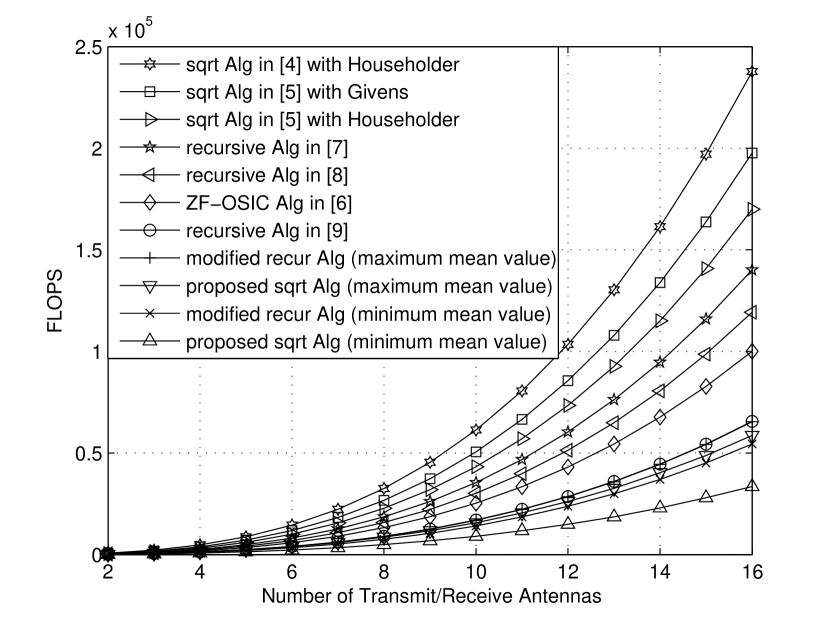
Assume $M=N$. For different number of transmit/receive antennas, we carried out some numerical experiments to count the average flops of the OSIC V-BLAST algorithms in [4, 7, 8, 9, 6, 5], the proposed square-root V-BLAST algorithm, and the recursive V-BLAST algorithm [9] with the above-described modification. The results are shown in Fig. 1. It can be seen that they are consistent with the theoretical flops calculation.

We propose a fast algorithm for inverse Cholesky factorization, to compute a triangular square-root of the estimation error covariance matrix for V-BLAST. Then it is employed to propose an improved square-root algorithm for V-BLAST, which speedups several steps in the previous one [5], and can offer further computational savings in MIMO OFDM systems. Compared to the conventional inverse Cholesky factorization, the proposed one avoids the back substitution (of the Cholesky factor), an inherent serial process unsuitable for the parallel implementation [18], and then requires only half divisions. The proposed V-BLAST algorithm is faster than the existing efficient V-BLAST algorithms in [4, 5, 6, 7, 10, 11, 8, 9]. Assume $M$ transmitters and the equal number of receivers. In MIMO OFDM systems, the expected speedups (in the number of flops) of the proposed square-root V-BLAST algorithm over the previous one [5] and the fastest known recursive V-BLAST algorithm [9] are $3.9\sim 5.2$ and $1.05\sim 1.4$, respectively. The recursive algorithm [9] can be modified to further reduce the complexity at the price of extra memory consumption, while the minimum expected complexity savings are negligible when $M$ is large. The speedups of the proposed square-root algorithm over the fastest known recursive algorithm [9] with the above-mentioned modification are $1.2$, when both algorithms are assumed to achieve the maximum complexity savings. Furthermore, as shown in [21], the proposed square-root algorithm can also be applied in the extended V-BLAST with selective per-antenna rate control (S-PARC), to reduce the complexity even by a factor of $M$.

References

- [1] G. J. Foschini and M. J. Gans, “On limits of wireless communications in a fading environment when using multiple antennas,” Wireless Personal Commun., pp. 311-335, Mar. 1998.
- [2] G. J. Foschini, “Layered space-time architecture for wireless communication in a fading environment using multi-element antennas,” Bell Labs. Tech. J.,, vol. 1, no. 2, pp. 41 C59, 1996.
- [3] P. W. Wolniansky, G. J. Foschini, G. D. Golden and R. A. Valenzuela, “V-BLAST: an architecture for realizing very high data rates over the rich-scattering wireless channel”, Proc. Int. Symp. Signals, Syst., Electron. (ISSSE 98), pp. 295-300, Sept. 1998.
- [4] B. Hassibi, “An efficient square-root algorithm for BLAST”, Proc. IEEE Int. Conf. Acoustics, Speech, and Signal Processing, (ICASSP ’00), pp. 737-740, June 2000.
- [5] H. Zhu, Z. Lei and F. P. S. Chin, “An improved square-root algorithm for BLAST”, IEEE Signal Processing Letters, vol. 11, no. 9, pp. 772-775, Sept. 2004.
- [6] W. Zha and S. D. Blostein, “Modified decorrelating decision-feedback detection of BLAST space-time system”, Proc. IEEE ICC, vol. 4, pp. 59-63, 2002.
- [7] J. Benesty, Y. Huang and J. Chen, “A fast recursive algorithm for optimum sequential signal detection in a BLAST system”, IEEE Trans. on Signal Processing, pp. 1722-1730, July 2003.
- [8] Z. Luo, S. Liu, M. Zhao and Y. Liu, “A Novel Fast Recursive MMSE-SIC Detection Algorithm for V-BLAST Systems”, IEEE Transactions on Wireless Communications, vol. 6, Issue 6, pp. 2022 - 2025, June 2007.
- [9] Y. Shang and X. G. Xia, “On Fast Recursive Algorithms For V-BLAST With Optimal Ordered SIC Detection”, IEEE Transactions on Wireless Communications, vol. 8, pp. 2860-2865, June 2009.
- [10] L. Szczeci nski, and D. Massicotte, “Low complexity adaptation of MIMO MMSE receivers, Implementation aspects”, Proc. IEEE Global Commun. Conf. (Globecom 05), St. Louis, MO, USA, Nov. 28 - Dec. 2, 2005.
- [11] H. Zhu, Z. Lei, and F. P. S. Chin, “An improved recursive algorithm for BLAST”, Signal Process., vol. 87, no. 6, pp. 1408-1411, Jun. 2007.
- [12] N. Boubaker, K.B. Letaief and R.D. Murch, “A low complexity multicarrier BLAST architecture for realizing high data rates over dispersive fading channels,” IEEE Vehicular Technology Conference (VTC), 2001 Spring, May 2001.
- [13] W. Yan, S. Sun and Z. Lei, “A low complexity VBLAST OFDM detection algorithm for wireless LAN systems”, IEEE Communications Letters, vol. 8, no. 6, pp. 374-376, June 2004.
- [14] G. H. Golub and C. F. Van Loan, Matrix Computations, Johns Hopkins University Press, Baltimore, MD, 3rd edition, 1996.
- [15] A. A. Rontogiannis and S. Theodoridis, “New fast QR decomposition least squares adaptive algorithms”, IEEE Trans. on Signal Processing, vol. 46, no. 8, pp. 2113-2121, Aug. 1998.
- [16] A. A. Rontogiannis, V. Kekatos and K. Berberidis, “A square-root adaptive V-BLAST algorithm for fast time-varying MIMO channels”, IEEE Signal Processing Letters, vol. 13, no. 5, pp. 265-268, May 2006.
- [17] A. Burian, J. Takala and M. Ylinen, “A fixed-point implementation of matrix inversion using Cholesky decomposition”, Micro-NanoMechatronics and Human Science, 2003 IEEE International Symposium on, 27-30 Dec. 2003, vol. 3, pp. 1431-1434.
- [18] E. J. Baranoski, “Triangular factorization of inverse data covariance matrices”, International Conference on Acoustics, Speech, and Signal Processing, 1991 (ICASSP-91), 14-17 Apr 1991, pp. 2245 - 2247, vol.3.
- [19] D. Bindel, J. Demmel, W. Kahan and O. Marques, “On Computing Givens rotations reliably and efficiently”, ACM Transactions on Mathematical Software (TOMS) archive, vol. 28 , Issue 2, June 2002. Available online at: www.netlib.org/lapack/lawns/downloads/.
- [20] B. Hassibi and H. Vikalo, “On the sphere decoding algorithm: Part I, the expected complexity”, IEEE Transactions on Signal Processing, vol 53, no 8, pages 2806-2818, Aug. 2005.
- [21] H. Zhu, W. Chen and B. Li, “Efficient Square-root Algorithms for the Extended V-BLAST with Selective Per-Antenna Rate Control”, IEEE Vehicular Technology Conference (VTC), 2010 Spring, May 2010.