An Inversion Formula for Horizontal Conical Radon Transform

Duy N. Nguyen¹¹1High School for the Gifted, Ho Chi Minh City, Vietnam. Email: nnduy@ptnk.edu.vn. and Linh V. Nguyen²²2University of Idaho, 875 Perimeter Dr, Moscow, ID 83844, USA. Email: lnguyen@uidaho.edu.

Abstract

In this paper, we consider the conical Radon transform on all cones with horizontal central axis whose vertices are on a straight line. We derive an explicit inversion formula for such transform. The inversion makes use of the vertical slice transform on a sphere and V-line transform on a plane.

1 Introduction

Let us denote by $\mathscr{C}$ the set all cones in $\mathbb{R}^{n}$ . Then, a (weighted) conical Radon transform of a function $f\in C^{\infty}(\mathbb{R}^{n})$ is the function $\mathbf{T}(f):\mathcal{M}\subset\mathscr{C}\to\mathbb{R}$ defined by

\mathbf{T}(f)(\mathbf{c})=\int_{\mathbf{c}}f(x)\,w(x,\mathbf{c})\,d\sigma(x),\quad c\in\mathcal{M},

where $w(x,\mathbf{c})$ is a positive smooth weight function. The conical Radon transform has been actively studied the thanks to its applications in Compton camera imaging (see, [6, 21]). In Compton camera imaging, one has to invert a conical Radon transform in order to find the interior image of a biological object from the measurement of Compton scattering.

In the two dimensional space ( $n=2$ ), the conical Radon transform becomes the V-line transform, which also arises in optical tomography [8]. There exist quite a few inversion formulas for the V-line transform (e.g. [3, 18, 23, 7, 2, 14]). In the three dimensional space ( $n=3$ ), $\mathscr{C}$ is a six dimensional manifold and there are many practical choices of $\mathcal{M}$ . Taking advantage of redundancy, i.e. by choosing $dim(\mathcal{M})>3$ , was the topic of several works (see, e.g., [22, 16]). One, however, may wish to study the case $dim(\mathcal{M})=3$ for the mathematical interest and practical setups for Compton camera imaging [5, 19, 1, 11, 17]. Several papers (e.g.,[10, 12, 22]) gave the inversion formula for conical transform in general dimensional space. We mention that using spherical harmonics to compute series solutions is also a popular approach for inversion (see, e.g., [4, 15, 20]).

Refer to caption — Figure 1: Our setups: the conical Radon transform over all cones with horizontal central line and the vertex in z-axis.

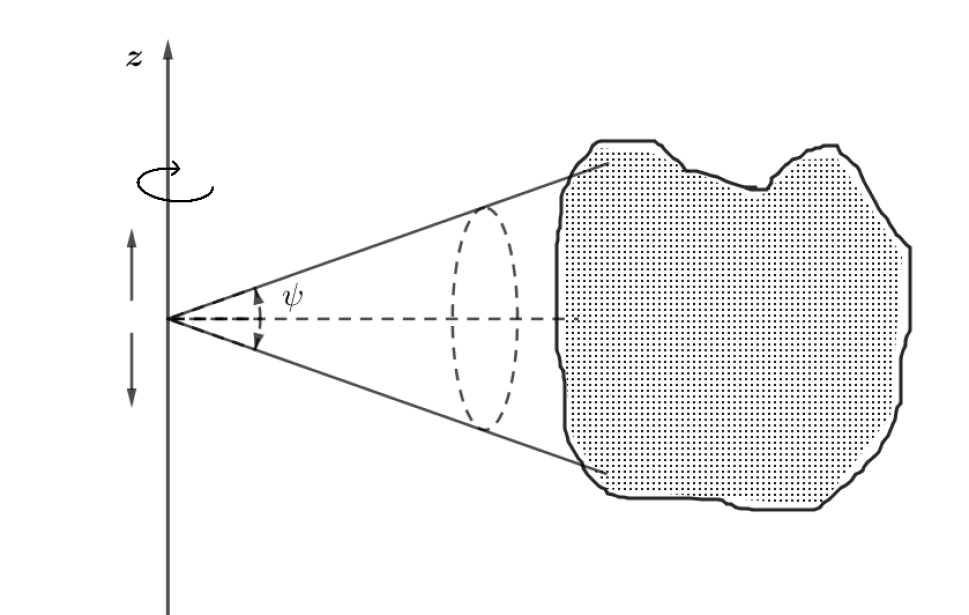
In this paper, we aim to reconstruct a function $f\in C^{\infty}(\mathbb{R}^{3})$ from all cones whose vertices are in a vertical line and central lines are horizontal, see Fig. 1. The manifold $\mathcal{M}$ of such cones is of three dimensions. This formulation corresponds to the Compton camera imaging with detectors on a line.

Let us now describe the problem in more detail. We introduce the following notations: $b\left(z\right)=\left(0,0,z\right)\in\mathbb{R}^{3}$ be a point in the $z$ -axis, ${{e}_{\varphi}}:=\left(\cos\varphi,\sin\varphi,0\right)$ is a horizontal unit vector in the $xyz$ -space, and

\mathbf{c}\left(z,\beta,\psi\right):=\left\{b\left(z\right)+r\omega|r\geq 0,\omega\in{{\mathbb{S}}^{2}},{{e}_{\beta}}\cdot\omega=\cos\psi\right\}

is the one-side circular cone, having vertex $b\left(z\right)$ and the symmetry axis $\left\{b(z)+r\cdot{{e}_{\beta}}|r>0\right\}$ .

We define our (weighted) conical Radon transform of a function $f\in C_{0}^{\infty}\left(\mathbb{R}^{3}\right)$ as follows.

	$\displaystyle\mathbf{T}_{k}(f)$	$\displaystyle:$	$\displaystyle\mathbb{R}\times\left[0,2\pi\right)\times\left(0,\frac{\pi}{2}\right)\longrightarrow\mathbb{R},$
			$\displaystyle\left(z,\beta,\psi\right)\longmapsto\int\limits_{\mathbf{c}\left(z,\beta,\psi\right)}{f\left(x\right){{\left\\|x-b\left(z\right)\right\\|}^{k-1}}dS\left(x\right)},$

where $k\in\mathbb{N}$ is fixed. In this paper, we investigate the inversion of $\mathbf{T}_{k}$ .

2 The main results

In order to invert the conical introduced in the previous section, we introduce the weighted X-ray and vertical slice transforms.

Definition 2.1 (The weighted X-Ray transform).

Let $k\in\mathbb{N}$ and $f\in C_{0}^{\infty}\left({\mathbb{R}^{3}}\right)$ . We define the weighted X-Ray transform

	$\displaystyle{{\chi}_{k}}f$	$\displaystyle:$	$\displaystyle\mathbb{R}\times({{\mathbb{R}}^{3}}\backslash\left\{0\right\})\longrightarrow\mathbb{R},$
	$\displaystyle\left(z,\omega\right)$	$\displaystyle\longmapsto$	$\displaystyle\int\limits_{0}^{\infty}{f\left(b\left(z\right)+r\omega\right){{r}^{k}}dr}.$

The weighted X-ray transform has been used in inverting the conical transform in other setups [17].

Definition 2.2 (The vertical slice transform).

Let $g\in C_{0}^{\infty}\left(\mathbb{S}^{2}\right)$ . We define the transform $\Gamma g:\left[0,2\pi\right)\times\mathbb{R}\longrightarrow\mathbb{R}$ by the formula

\displaystyle\Gamma g\left(\varphi,t\right)=\left\{\begin{array}[]{l}\frac{1}{2\pi\sqrt{1-{{t}^{2}}}}\int\limits_{{{e}_{\varphi}}\cdot\omega=t}{g\left(\omega\right)\,d\omega},\mbox{ for }-1<t<1,\\[12.0pt] g\left(\pm e_{\varphi}\right),\mbox{ for }t=\pm 1,\\[6.0pt] 0,\mbox{ for }|t|>1.\end{array}\right.

Vertical slice transform was investigated Gindikin [9]. It has the following inversion formula (see [9, Theorem 2.1]):

Theorem 2.3.

Let $\omega\in\mathbb{S}^{2}$ and $g:C(\mathbb{S}^{2})\longrightarrow\mathbb{R}$ is even in the third coordinate. Then

g\left(\omega\right)=\dfrac{-\sqrt{1-\omega_{1}^{2}-\omega_{2}^{2}}}{4\pi}\int\limits_{-\infty}^{+\infty}\dfrac{1}{t}\int\limits_{0}^{2\pi}\dfrac{\partial}{\partial t}\Gamma g\left(\varphi,\omega_{1}\cos\varphi+\omega_{2}\sin\varphi+t\right)\,d\varphi\,dt.

(2)

The following lemma gives us the relationship between the weighted $X$ -ray, the weighted conical Radon, and the vertical slice transforms:

Lemma 2.4.

For every $k\in\mathbb{N}$ and $f\in C_{0}^{\infty}\left(\mathbb{R}^{3}\right)$ , $z\in\mathbb{R},\beta\in\left[0,2\pi\right),\psi\in\left(0,\pi\right)$ then

\Gamma\left(\chi_{k}f\right)\left(z,\beta,\cos\psi\right)=\dfrac{\mathbf{T}_{k}(f)\left(z,\beta,\psi\right)}{2\pi\sin^{2}\psi}.

(3)

In the lemma, we have used the notation $\Gamma(\chi_{k}f)(z,\cdot)$ for the vertical slice transform of $\chi_{k}f(z,\cdot)$ . Let us now prove the lemma.

Proof.

We have

	$\displaystyle\mathbf{T}_{k}(f)\left(z,\beta,\psi\right)$	$\displaystyle=\int\limits_{\mathbf{c}\left(\varphi,z,\beta,\psi\right)}{f\left(x\right){{\left\\|x-b\left(z\right)\right\\|}^{k-1}}\,d\sigma\left(x\right)}=\sin\psi\int\limits_{{\mathbb{S}^{2}}}{\int\limits_{0}^{\infty}{f\left(b\left(z\right)+r\omega\right){{r}^{k}}\delta\left({{e}_{\beta}}\cdot\omega-\cos\psi\right)\,dr\,d\sigma\left(\omega\right)}}$
		$\displaystyle=\sin\psi\int\limits_{{{\mathbb{S}}^{2}}}{{{\chi}_{k}}f\left(z,\omega\right)\delta\left({{e}_{\beta}}\cdot\omega-\cos\psi\right)dS\left(\omega\right)}=2\pi{{\sin}^{2}}\left(\psi\right)\Gamma\left(\chi_{k}f\right)\left(z,\beta,\cos\psi\right).$

This finishes the proof. ∎

For any $\omega=\left(\omega_{1},\omega_{2},\omega_{3}\right)\in\mathbb{R}^{3}$ , we define the even and odd parts of the function $\chi_{k}f$ as follows:

	$\displaystyle(\chi_{k}f)_{e}\left(z,\omega\right)$	$\displaystyle=$	$\displaystyle\dfrac{\chi_{k}f\left(z,\omega_{1},\omega_{2},\omega_{3}\right)+\chi_{k}f\left(z,\omega_{1},\omega_{2},-\omega_{3}\right)}{2},$
	$\displaystyle(\chi_{k}f)_{o}\left(z,\omega\right)$	$\displaystyle=$	$\displaystyle\dfrac{\chi_{k}f\left(z,\omega_{1},\omega_{2},\omega_{3}\right)-\chi_{k}f\left(z,\omega_{1},\omega_{2},-\omega_{3}\right)}{2}.$

Notice that $\chi_{k}f\left(z,\omega\right)=(\chi_{k}f)_{e}\left(z,\omega\right)+(\chi_{k}f)_{o}\left(z,\omega\right)$ . Since all the circles appearing in the vertical slice transform are symmetric with respect to the $xy$ -plane and $(\chi_{k}f)_{o}$ is an odd function in the third coordinate, $\Gamma(\chi_{k}f_{o})\equiv 0$ . Therefore, from Lemma 2.4, we obtain

\Gamma(\chi_{k}f)_{e}\left(z,\beta,\cos\psi\right)=\Gamma(\chi_{k}f)\left(z,\beta,\cos\psi\right)=\dfrac{\mathbf{T}_{k}(f)\left(z,\beta,\psi\right)}{2\pi\,{{\sin}^{2}}\psi}.

(4)

Let $a\left(\varphi,\eta\right):=\left(\cos\varphi\sin\eta,\sin\varphi\sin\eta,\cos\eta\right)\in{{\mathbb{S}}^{2}}$ be the unit vector in $\mathbb{R}^{3}$ determined by the horizontal angle $\varphi$ and vertical angle $\eta$ . We denote $(\chi_{k}f)_{e}\left(z,\varphi,\eta\right)=(\chi_{k}f)_{e}\left(z,a\left(\varphi,\eta\right)\right)$ , then:

Lemma 2.5.

For $k\in\mathbb{N}$ , $f\in C_{0}^{\infty}\left(\mathbb{R}^{3}\right)$ , $z\in\mathbb{R}$ , $\varphi\in\left[0,2\pi\right]$ , $\eta\in\left(0,\pi\right)$ ,

	$\displaystyle(\chi_{0}f)_{e}$	$\displaystyle\left(z,\varphi,\eta\right)=\dfrac{1}{8\pi^{2}(k-1)!}\int\limits_{\eta}^{\pi}\dfrac{\sin^{k-1}\left(\gamma-\eta\right)}{\sin^{k}\eta}\left\|\cos\gamma\right\|$
		$\displaystyle\times\left\{\int\limits_{0}^{2\pi}\left[\int\limits_{0}^{\pi}\dfrac{1}{\cos\psi-\sin\gamma\cos\left(\beta-\varphi\right)}\partial_{z}^{k}\left(\dfrac{\partial}{\partial\psi}\left(\dfrac{\mathbf{T}_{k}f\left(z,\beta,\psi\right)}{\sin^{2}\psi}\right)\right)d\psi\right]d\beta\right\}d\gamma.$		(5)

Proof.

Since $(\chi_{k}f)_{e}$ is even in the third coordinate, applying Lemma 2.4 and Theorem 2.3, we obtain

\displaystyle(\chi_{k}f)_{e}\left(z,\omega\right)

\displaystyle=\dfrac{-\sqrt{1-\omega_{1}^{2}-\omega_{2}^{2}}}{4\pi}\int\limits_{-\infty}^{+\infty}\dfrac{1}{q}\int\limits_{0}^{2\pi}\dfrac{\partial}{\partial q}\Gamma\left(\chi_{k}f_{e}\right)\left(z,\beta,\omega_{1}\cos\beta+\omega_{2}\sin\beta+q\right)d\beta dq.

For any $\omega\in{\mathbb{S}}^{2}$ , we can write $\omega=a(\varphi,\eta)=\left(\sin\eta\cos\varphi,\sin\eta\sin\varphi,\cos\eta\right)$ . Therefore,

\displaystyle(\chi_{k}f)_{e}\left(z,\omega\right)

\displaystyle=\dfrac{-\sqrt{1-\sin^{2}\eta}}{4\pi}\int\limits_{0}^{2\pi}\int\limits_{-\infty}^{+\infty}\dfrac{1}{q}\dfrac{\partial}{\partial q}\Gamma\left(\chi_{k}f_{e}\right)\left(z,\beta,\sin\eta\cos\left(\beta-\varphi\right)+q\right)dqd\beta.

Since $\Gamma(\chi_{k}f)_{e}\left(.,t\right)=0$ when $|t|>1$ , we only need to consider when the third variable in the integrand is in the interval $[-1,1]$ . We, hence, can define $\cos\psi=\sin\eta\cos\left(\beta-\varphi\right)+q$ for some $\psi\in[0,\pi]$ . We arrive at

\displaystyle(\chi_{k}f)_{e}\left(z,\varphi,\eta\right)

\displaystyle=\dfrac{\left|\cos\eta\right|}{4\pi}\int\limits_{0}^{2\pi}\int\limits_{0}^{\pi}\dfrac{1}{\cos\psi-\sin\eta\cos\left(\beta-\varphi\right)}\dfrac{\partial}{\partial\psi}\Gamma\left(\chi_{k}f_{e}\right)\left(z,\beta,\cos\psi\right)d\psi d\beta.

Using (4), we deduce

\displaystyle(\chi_{k}f)_{e}\left(z,\varphi,\eta\right)

\displaystyle=\dfrac{\left|\cos\eta\right|}{4\pi}\int\limits_{0}^{2\pi}\int\limits_{0}^{\pi}\dfrac{1}{\cos\psi-\sin\eta\cos\left(\beta-\varphi\right)}\dfrac{\partial}{\partial\psi}\left(\dfrac{\mathbf{T}_{k}(f)\left(z,\beta,\psi\right)}{2\pi\sin^{2}\psi}\right)d\psi d\beta.

On the other hand (see, e.g., [17]),

	$\displaystyle(\chi_{0}f)_{e}\left(z,\omega_{1},\omega_{2},\omega_{3}\right)$	$\displaystyle=\dfrac{1}{(k-1)!}\int\limits_{-\infty}^{\omega_{3}}\left(\omega_{3}-s\right)^{k-1}\partial_{z}^{k}\left(\chi_{k}f_{e}\right)\left(z,\omega_{1},\omega_{2},s\right)ds$
		$\displaystyle=\dfrac{1}{(k-1)!}\int\limits_{-\infty}^{\omega_{3}}\left(\omega_{3}-s\right)^{k-1}\partial_{z}^{k}\left(\chi_{k}f_{e}\right)\left(z,\left(\dfrac{\omega_{1},\omega_{2},s}{h}\right)\right)h^{-(k+1)}ds,$

for any $h>0$ .

Let us change the variable $s\to\gamma$ by the formula $s=\cot\gamma\sin\eta,\,\gamma\in\left(0,\pi\right)$ . Then, $ds=\dfrac{-\sin\eta}{\sin^{2}\gamma}d\gamma$ . Choosing $h=\dfrac{\sin\eta}{\sin\gamma}$ ,

	$\displaystyle(\chi_{0}f)_{e}\left(z,\varphi,\eta\right)=$	$\displaystyle\dfrac{1}{(k-1)!}\int\limits_{\eta}^{\pi}\left(\cos\eta-\sin\eta\cot\gamma\right)^{k-1}\partial_{z}^{k}\left(\chi_{k}f_{e}\right)\left(z,\left(\sin\gamma\theta\left(\varphi\right),\cos\gamma\right)\right)\left(\dfrac{\sin\gamma}{\sin\eta}\right)^{k+1}\dfrac{\sin\eta}{\sin^{2}\gamma}d\gamma$
	$\displaystyle=$	$\displaystyle\dfrac{1}{(k-1)!}\int\limits_{\eta}^{\pi}\dfrac{\sin^{k-1}\left(\gamma-\eta\right)}{\sin^{k}\eta}\partial_{z}^{k}\left(\chi_{k}f_{e}\right)\left(z,\left(\sin\gamma\theta\left(\varphi\right),\cos\gamma\right)\right)d\gamma$
	$\displaystyle=$	$\displaystyle\dfrac{1}{(k-1)!}\int\limits_{\eta}^{\pi}\dfrac{\sin^{k-1}\left(\gamma-\eta\right)}{\sin^{k}\eta}$
		$\displaystyle\times\partial_{z}^{k}\left\{\dfrac{\left\|\cos\gamma\right\|}{4\pi}\int\limits_{0}^{2\pi}\int\limits_{0}^{\pi}\dfrac{1}{\cos\psi-\sin\gamma\cos\left(\beta-\varphi\right)}\dfrac{\partial}{\partial\psi}\left(\dfrac{\mathbf{T}_{k}(f)\left(z,\beta,\psi\right)}{2\pi\sin^{2}\psi}\right)d\psi d\beta\right\}d\gamma$
	$\displaystyle=$	$\displaystyle\dfrac{1}{8\pi^{2}(k-1)!}\int\limits_{\eta}^{\pi}\dfrac{\sin^{k-1}\left(\gamma-\eta\right)}{\sin^{k}\eta}\left\|\cos\gamma\right\|$
		$\displaystyle\times\left\{\int\limits_{0}^{2\pi}\left[\int\limits_{0}^{\pi}\dfrac{1}{\cos\psi-\sin\gamma\cos\left(\beta-\varphi\right)}\partial_{z}^{k}\left(\dfrac{\partial}{\partial\psi}\left(\dfrac{\mathbf{T}_{k}(f)\left(z,\beta,\psi\right)}{\sin^{2}\psi}\right)\right)d\psi\right]d\beta\right\}d\gamma$

This finishes our proof. ∎

Let us note $2(X_{0}f)_{e}(z,\varphi,\eta)$ is the integral of $f$ along a V-line whose vertex is $b(z)$ , each branch makes an angle $\eta$ to the horizontal plane and is the reflection of the other via the horizontal plane. We are now ready to compute the function $f$ in $\mathbb{R}^{3}$ from its conical transform in Definition 2.1. To this end, we will decompose $\mathbb{R}^{3}$ into the union of half-planes $\mathbb{H}_{\vec{e}}$ , where $\vec{e}$ is a horizontal unit vector. Here, $\mathbb{H}_{\vec{e}}$ is the vertical half plane passing through the $z$ -axis and containing the unit vector $\vec{e}$ . We only need to compute $f$ on each such half-plane. On each such half-plane we are given the V-line transform of the function $f$ , which integrates $f$ over all V-lines with horizontal central axis whose vertices are on the boundary of $\mathbb{H}_{\vec{e}}$ . The inversion such transform can be reduced to that of the X-ray transform (see [3]). The idea will be used in our proof below for Theorem 2.6 below.

Theorem 2.6 (Inversion Formula of Conical Radon Transform).

For each $x\in\mathbb{R}^{3}$ , we write $x=\left(re_{\varphi},x_{3}\right)$ where $r\geq 0$ and $\varphi\in\left[0,2\pi\right)$ . Then,

	$\displaystyle f\left(x\right)$	$\displaystyle=\dfrac{1}{8\pi^{4}(k-1)!}\int\limits_{0}^{\pi}\int_{\mathbb{R}}\dfrac{1}{r\cos\eta+x_{3}\sin\eta-p}$
		$\displaystyle\times\left\{\int\limits_{\eta}^{\pi}\sin^{k-1}\left(\gamma-\eta\right)\|\cos\gamma\|\int\limits_{0}^{2\pi}\left[\int\limits_{0}^{\pi}\dfrac{\partial_{p}^{k+1}\left[\partial_{\psi}\left(\dfrac{\mathbf{T}_{k}(f)\left(p/\sin\eta,\beta,\psi\right)}{\sin^{2}\psi}\right)\right]}{\cos\psi-\sin\gamma\cos\left(\beta-\varphi\right)}d\psi\right]d\beta\right\}\,d\gamma\,dp\,d\eta.$

Proof.

Let $\mathbb{H}$ be the vertical half-plane passing through the z-axis and the unit vector $\vec{e}=e_{\varphi}$ . For any $x\in\mathbb{H}$ then $x=\left(r\theta\left(\varphi\right),x_{3}\right)$ . We define $f^{*}\left(r,x_{3}\right)=f\left(r\theta\left(\varphi\right),x_{3}\right),\mbox{ for }r\geq 0$ . We then extend $f^{*}$ to the whole space $(r,x_{3})\in\mathbb{R}^{2}$ by the even reflection. Then, for any $\eta\in(0,\pi),p\in\mathbb{R}$ , we have

\displaystyle(\chi_{0}f)_{e}\left(z,\varphi,\eta\right)=\dfrac{1}{2}\int\limits_{-\infty}^{+\infty}f^{*}\left(r\sin\eta,z-r\cos\eta\right)dr=\dfrac{1}{2}\mathbf{R}(f^{*})\left(\eta,z\sin\eta\right).

Here, $\mathbf{R}$ denote the standard Radon transform in two dimensional space. Choosing $z=\dfrac{p}{\sin\eta}$ , then

\mathbf{R}(f^{*})\left(\eta,p\right)=2(\chi_{0}f)_{e}\left(\dfrac{p}{\sin\eta},\varphi,\eta\right),\mbox{ for }0<\eta<\pi.

Since $f\in C_{0}^{\infty}\left(\mathbb{R}^{3}\right)$ , the value of $\mathbf{R}(f^{*})$ at $\eta=0,\pi$ can be computed by the continuous extension. Now, using the inversion of the Radon transform (see [13]) and Lemma 2.5, we conclude

	$\displaystyle f^{*}\left(r,x_{3}\right)$	$\displaystyle=\dfrac{1}{2\pi^{2}}\int\limits_{0}^{\pi}\int_{\mathbb{R}}\dfrac{\partial_{p}\mathbf{R}f^{*}\left(\eta,p\right)}{r\cos\eta+x_{3}\sin\eta-p}dpd\eta=\dfrac{1}{\pi^{2}}\int\limits_{0}^{\pi}\int_{\mathbb{R}}\dfrac{\partial_{p}\left(\chi_{0}f_{e}\right)\left(\dfrac{p}{\sin\eta},\varphi,\eta\right)}{r\cos\eta+x_{3}\sin\eta-p}dpd\eta$
		$\displaystyle=\dfrac{1}{8\pi^{4}(k-1)!}\int\limits_{0}^{\pi}\int_{\mathbb{R}}\dfrac{1}{r\cos\eta+x_{3}\sin\eta-p}$
		$\displaystyle\times\left\{\int\limits_{\eta}^{\pi}\sin^{k-1}\left(\gamma-\eta\right)\|\cos\gamma\|\int\limits_{0}^{2\pi}\left[\int\limits_{0}^{\pi}\dfrac{\partial_{p}^{k+1}\left[\partial_{\psi}\left(\dfrac{\mathbf{T}_{k}(f)\left(p/\sin\eta,\beta,\psi\right)}{\sin^{2}\psi}\right)\right]}{\cos\psi-\sin\gamma\cos\left(\beta-\varphi\right)}d\psi\right]d\beta\right\}d\gamma dpd\eta.$

This finishes our proof. ∎

Acknowlegement

Linh Nguyen’s research is partially supported by the NSF grants, DMS 1212125 and DMS 1616904.

References

[1] Moritz Allmaras, David P Darrow, Yulia Hristova, Guido Kanschat, and Peter Kuchment. Detecting small low emission radiating sources. arXiv preprint arXiv:1012.3373, 2010.
[2] Gaik Ambartsoumian. Inversion of the v-line radon transform in a disc and its applications in imaging. Computers & Mathematics with Applications, 64(3):260–265, 2012.
[3] Roman Basko, Gengsheng L Zeng, and Grant T Gullberg. Analytical reconstruction formula for one-dimensional compton camera. IEEE Transactions on Nuclear Science, 44(3):1342–1346, 1997.
[4] Roman Basko, Gengsheng L Zeng, and Grant T Gullberg. Application of spherical harmonics to image reconstruction for the compton camera. Physics in Medicine & Biology, 43(4):887, 1998.
[5] Michael J Cree and Philip J Bones. Towards direct reconstruction from a gamma camera based on compton scattering. IEEE transactions on medical imaging, 13(2):398–407, 1994.
[6] DB Everett, JS Fleming, RW Todd, and JM Nightingale. Gamma-radiation imaging system based on the compton effect. In Proceedings of the Institution of Electrical Engineers, volume 124, pages 995–1000. IET, 1977.
[7] Lucia Florescu, Vadim A Markel, and John C Schotland. Inversion formulas for the broken-ray radon transform. Inverse Problems, 27(2):025002, 2011.
[8] Lucia Florescu, John C Schotland, and Vadim A Markel. Single-scattering optical tomography. Physical Review E, 79(3):036607, 2009.
[9] S Gindikin, J Reeds, and L Shepp. Spherical tomography and spherical integral geometry. Tomography, Impedance Imaging, and Integral Geometry (South Hadley, MA, 1993), Lectures in Appl. Math, 30:83–92, 1994.
[10] Rim Gouia-Zarrad. Analytical reconstruction formula for n-dimensional conical radon transform. Computers & Mathematics with Applications, 68(9):1016–1023, 2014.
[11] Rim Gouia-Zarrad and Gaik Ambartsoumian. Exact inversion of the conical radon transform with a fixed opening angle. Inverse Problems, 30(4):045007, 2014.
[12] Markus Haltmeier. Exact reconstruction formulas for a radon transform over cones. Inverse Problems, 30(3):035001, 2014.
[13] Sigurdur Helgason and S Helgason. The radon transform, volume 2. Springer, 1999.
[14] Yulia Hristova. Inversion of a v-line transform arising in emission tomography. Journal of Coupled Systems and Multiscale Dynamics, 3(3):272–277, 2015.
[15] Chang-Yeol Jung and Sunghwan Moon. Inversion formulas for cone transforms arising in application of compton cameras. Inverse Problems, 31(1):015006, 2015.
[16] Peter Kuchment and Fatma Terzioglu. Three-dimensional image reconstruction from compton camera data. SIAM Journal on Imaging Sciences, 9(4):1708–1725, 2016.
[17] Sunghwan Moon and Markus Haltmeier. Analytic inversion of a conical radon transform arising in application of compton cameras on the cylinder. SIAM Journal on imaging sciences, 10(2):535–557, 2017.
[18] Marcela Morvidone, Maï Khuong Nguyen, Tuong T Truong, and Habib Zaidi. On the v-line radon transform and its imaging applications. Journal of Biomedical Imaging, 2010:11, 2010.
[19] Mai K Nguyen, Tuong T Truong, and Pierre Grangeat. Radon transforms on a class of cones with fixed axis direction. Journal of Physics A: Mathematical and General, 38(37):8003, 2005.
[20] Daniela Schiefeneder and Markus Haltmeier. The radon transform over cones with vertices on the sphere and orthogonal axes. SIAM Journal on Applied Mathematics, 77(4):1335–1351, 2017.
[21] Manbir Singh. An electronically collimated gamma camera for single photon emission computed tomography. part i: Theoretical considerations and design criteria. Medical Physics, 10(4):421–427, 1983.
[22] Fatma Terzioglu. Some inversion formulas for the cone transform. Inverse Problems, 31(11):115010, 2015.
[23] Tuong T Truong and Mai K Nguyen. On new v-line radon transforms in $\mathbb{R}^{2}$ and their inversion. Journal of Physics A: Mathematical and Theoretical, 44(7):075206, 2011.