An Inversion Tool for Conditional Term Rewriting Systems – A Case Study of Ackermann Inversion

	remove-index	rem(:(x,xs),0) -> <x,xs> rem(:(x,xs),s(i)) -> <y,:(x,zs)> <= rem(xs,i) -> <y,zs>
$\xRightarrow{\text{\footnotesize{Full inv.}}}$	random-insert	rem{}{1,2}(x,xs) -> <:(x,xs),0> rem{}{1,2}(y,:(x,zs)) -> <:(x,xs),s(i)> <= rem{}{1,2}(y,zs) -> <xs,i>
$\xRightarrow{\text{\footnotesize{Partial inv.}}}$	insert	rem{2}{1,2}(0,x,xs) -> <:(x,xs)> rem{2}{1,2}(s(i),y,:(x,zs)) -> <:(x,xs)> <= rem{2}{1,2}(i,y,zs) -> <xs>
$\xRightarrow{\text{\footnotesize{Semi-inv.}}}$	remove-elem	rem{1}{1}(:(x,xs),x) -> <0,xs> rem{1}{1}(:(x,xs),y) -> <s(i),:(x,zs)> <= rem{1}{1}(xs,y) -> <i,zs>

Let us illustrate our tool with three kinds of inversions of a simple remove-index function, rem (Figure 1). Given a list and a unary number $n$ , it returns the $n$ th element of the list and the list without the removed element. rem is defined by two rewrite rules: the first rule defines the base case where cons (:) is written in prefix notation and the two outputs are tupled (< $\cdot$ >). The second rule contains a so-called condition after the separator (<=) that can be read as a recursion. The input-output relation specified by rem is exemplified by the list $[a,b,b]$ and the indices 0, 1, and 2 (inputs are marked in blue).

Usually, we consider program inversion as full inversion that swaps a program’s entire input and output. In our tool, the new directionality of the desired program is specified by input and output index sets (io-sets). The user can select the input and output arguments that become the input arguments of the inverse program, so this technique is very general. Full inversion always has an empty input index set $I$ and an output index set $O$ containing all indices of the outputs.

Full inversion of rem yields a program rem{}{1,2} whose non-functional input-output relation specifies the insertion of an element into a list at an arbitrary position. The updated lists and the corresponding positions are the output. The name rem{}{1,2} indicates that none of rem’s inputs ({}) and all of rem’s outputs ({1,2}) are the new inputs.

The full inverse of a non-injective function specifies a non-functional relation. Thus, program inversion does not respect language paradigms, and this is one of the inherent difficulties when performing program inversion for a functional language. The inverted rules do not always define a functional relation because they may have overlapping left-hand sides or extra variables. The non-functional relation random-insert of rem{}{1,2} is induced by two overlapping rules.

Partial inversion swaps parts of the input and the entire output. rem{2}{1,2} is a partial inverse of rem where the original list is swapped with the entire output. It defines the insertion of an element at a position $n$ in a list, i.e., the functional relation insert. Semi-inversion, the most general form of inversion, can swap any part of the input and output. rem{1}{1} is a semi-inversion of rem where the position and the element are swapped, i.e., the non-functional relation remove-elem. While we obtain two programs for the price of one by full inversion, we can obtain several programs by partial and semi-inversion.

{myverbbox}

[]\ccsadd add(0,y) -¿ ¡y¿ add(s(x),y) -¿ ¡s(z)¿ ¡= add(x,y) -¿ ¡z¿

{myverbbox}

[]\ccsaddinv add11(0,y) -¿ ¡y¿ add11(s(x),s(z)) -¿ ¡y¿ ¡= add11(x,z) -¿ ¡y¿

Figure 2: The tool illustrated with the partial inversion of add defining the addition of unary numbers.

The contribution of the work reported here is a complete implementation of the generic inversion algorithm, together with four well-behaved rule inverters. The system is available for experimental (source code) and educational purposes (web system). We then report on the case study of Ackermann inversion repeating three experiments by A.Y. Romanenko and compare the results and provide measures of the rewrite steps and function calls. We are not aware of other investigations of Romanenko’s experiments.

We begin by giving an overview of the tool (Section 2) followed by the case study of Ackermann inversion (Section 3). This paper, the tool implementation itself, and the paper on the inversion framework are intended to complement each other. They are intended to be used together. For more details on the generic inversion algorithm and the rule inverters, interested readers are therefore referred to [7].

2 Inversion Tool

The tool is implemented in Haskell²²2The Glorious Glasgow Haskell Compilation System, version 8.10.4, and we provide both an online web-based version³³3https://topps.di.ku.dk/pirc/inversion-tool and the source code⁴⁴4https://github.com/pirc-src/inversion-tool. We demonstrate how to partially invert a function add, which defines the addition of two unary numbers, to obtain add{1}{1}, which defines the subtraction of two unary numbers. As illustrated in Figure 2, the Inversion Framework requires three inputs: (i) the original CCS rules with the add-rules, (ii) the Inversion task: add with io-set $I=\{1\}$ and $O=\{1\}$ , and (iii) an indication of which well-behaved Rule inverter the tool should apply, here, the partial rule inverter. The inversion framework provides two outputs: (i) the Inverted CCS rules, containing the add{1}{1}-rules defining subtraction, and (ii) a Diagnostics table with an overview of the systems’ paradigm characteristics. Because the program inversion does not respect language paradigms, it is useful that the tool also provides an analysis of the programs’ paradigm characteristics; see [7, Fig.2] for definitions and interrelations.

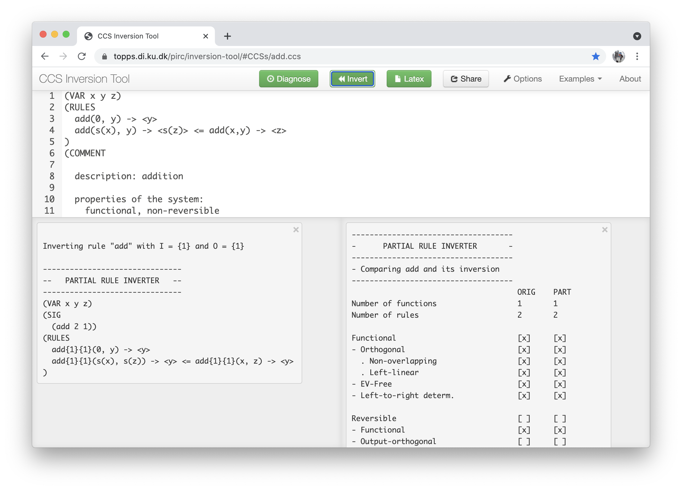
Refer to caption — Figure 3: The interface of the web-based inversion tool after partially inverting add to add{1}{1}.

Whereas the source code provides a command line interface, which facilitates composition with other program transformations, the online web-based version provides a friendly clickable interaction; see Figure 3 for a screenshot. In the following, we describe the most important content and features of the online tool. The tool web-site contains the following:

1.

a navigation bar (in the top) with green action buttons and white settings buttons,
2.

a white input window with a text field for the original CCS,
3.

a gray output window (in the lower left corner) for the inverted systems, and
4.

another gray output window (in the lower right corner) with program diagnostics.

The original CCS can either be entered into the input window or chosen from the predefined CCS examples available via the Examples button, e.g., choosing add. Using the Options button, one defines the inversion task, e.g., the partial inversion of add with $I=\{1\}$ and $O=\{1\}$ and selects one of the rule inverters, e.g., the partial rule inverter. To apply the inverter, we use the Invert button whereafter the tool creates (or updates) the gray output windows with the inversion, e.g., the partial inversion add{1}{1}, and the paradigm characteristics of both the original and the inverted program, e.g., column ORIG and column PART. For instance, we can see that both add and add{1}{1} are functional and that none of them is reversible. The Diagnose button provides a more detailed property analysis of the program in the white input text field. Another feature is the Latex button that translates the CCS in the main window into LaTeX code that can be used when typesetting documents.

ack(0,y)       -> <s(y)>
ack(s(x),0)    -> <z> <= ack(x,s(0)) -> <z>
ack(s(x),s(y)) -> <z> <= ack(s(x),y) -> <v>, ack(x,v) -> <z>

(a) Program ack implementing the Ackermann function

\mathit{Ack}(x,y)

.

ack{1}{1}(0,s(y)) -> <y>
ack{1}{1}(s(x),z) -> <0>    <= ack{1,2}{1}(x,s(0),z) -> <>
ack{1}{1}(s(x),z) -> <s(y)> <= ack{1}{1}(x,z)    -> <v>,
                               ack{1}{1}(s(x),v) -> <y>
ack{1,2}{1}(0,y,s(y))    -> <>
ack{1,2}{1}(s(x),0,z)    -> <> <= ack{1,2}{1}(x,s(0),z) -> <>
ack{1,2}{1}(s(x),s(y),z) -> <> <= ack{1}{1}(x,z) -> <v>,
                                  ack{1,2}{1}(s(x),y,v) -> <>

(b) Partial inverse of ack with

I=\{1\}

and

O=\{1\}

.

ack_2(0,s(y)) -> <y>
ack_2(s(x),z) -> <0>    <= ack_2(x,z) -> <s(0)>
ack_2(s(x),z) -> <s(y)> <= ack_2(x,z) -> <v>,
                           ack_2(s(x),v) -> <y>

(c) Romanenko’s partial inverse

\mathit{Ack}_{\_}2^{-1}

[17, p.17] rewritten as a CCS.

Figure 4: Partial inversions of the Ackermann function and the dependency graphs.

3 A Case Study of Ackermann Inversion

We illustrate the use of our tool by repeating three experiments [17], namely, two partial inversions and a full inversion of the Ackermann function ack (Figure 4(a)). ack takes two unary numbers as inputs and returns one unary number as output.

First Experiment

An io-set together with the ack program in Figure 4(a) are the tool inputs. The io-set for this experiment is $I=\{1\}$ and $O=\{1\}$ , specifying that the first input term and the output term of ack are the inputs for the partially inverted program ack{1}{1}. Then, our tool propagates the io-set through the entire program and transforms the rules locally using the selected well-behaved rule inverter.

The result of the pure partial inversion [7, Fig.6] is shown in Figure 4(b). The resulting program consists of two defined function symbols, namely, the desired partial inverse ack{1}{1}, which depends on another partial inverse ack{1,2}{1}. The io-set of ack{1,2}{1} specifies that it takes both inputs and the output of ack as the input. As a consequence, all of its three rules return a nullary output tuple <>. In the case of Romanenko’s ack_2 in Figure 4(c), the second rule’s right-hand side of the condition is a constant s(0). Since this output is a known constant, we can provide it as input to the left-hand side using our tool. This illustrates that our tool fully propagates the io-sets such that all known terms become the new input. This means that the algorithm is a polyvariant inverter in that it may produce several inversions of the same function symbol, namely, one for each input-output index set.

The relation specified by the partial inverse is functional [17, p.18], but the program in Figure 4(b) is nondeterministic due to a single pair of overlapping rules, i.e., the 2nd and 3rd rules of ack{1}{1}. The same issue occurs for the partially inverted program $\mathit{Ack}_{\_}2^{-1}$ (ack2, Figure 4(c)) [17, p.17]. Comparison of the two programs shows that in ack{1}{1}’s second rule, our tool has moved the condition’s constant s(0) to the input side and thereby created a dependency on the more specific partial inversion ack{1,2}{1} instead of ack{1}{1}.

The effect is to reduce the search space when rewriting using the inverted systems. In this experiment, we found a remarkable reduction of function calls and rewrite steps. The results and the speed-ups for ack2 and ack{1}{1} are reported in Table 1. For the tested inputs ranging from (1, 2) to (3, 509) the speed-up is up to 5.89 for rewrite steps and up to 3.92 for function calls when comparing ack{1}{1} with Romanenko’s ack2. We observe that there is a rewrite step speed-up for all inputs, while the two programs have equally many function calls when the first input is 1. One reason is that ack{1}{1} tends to use fewer rewriting steps because its call to ack{1,2}{1} can fail using pattern matching, whereas ack2 requires a rewriting and pattern match of the result to establish the same failure.

The number of required rewrite steps is used in the complexity of conditional term rewriting systems [9], and the number of function/predicate calls is used in the complexity analysis of functional and logic programs [10, 12]. Here, function calls correspond to the number of function-rooted terms that must be rewritten to reach normal form.

Input		(1, 2)	(1, 3)	(1, 4)	(1, 5)	(1, 6)	(1, 7)	(1, 8)
ack_2	Rewrite steps	5	8	11	14	17	20	23
	Function calls	9	12	15	18	21	24	27
ack{1}{1}	Rewrite steps	4	6	8	10	12	14	16
	Function calls	9	12	15	18	21	24	27
Speed-up	Rewrite steps	1.25	1.33	1.38	1.40	1.42	1.43	1.53
	Function calls	1.00	1.00	1.00	1.00	1.00	1.00	1.00
Input		(2, 3)	(2, 5)	(2, 7)	(2, 9)	(2, 11)	(2, 13)	(2, 15)
ack_2	Rewrite steps	21	50	91	144	209	286	375
	Function calls	38	75	124	185	258	343	440
ack{1}{1}	Rewrite steps	13	25	41	61	85	113	145
	Function calls	28	51	80	115	156	203	256
Speed-up	Rewrite steps	1.62	2.00	2.22	2.36	2.46	2.53	2.59
	Function calls	1.36	1.47	1.55	1.61	1.65	1.69	1.72
Input		(3, 5)	(3, 13)	(3, 29)	(3, 61)	(3, 125)	(3, 253)	(3, 509)
ack_2	Rewrite steps	109	682	3351	14820	62321	255614	1035403
	Function calls	178	865	3776	15743	64254	259581	1043452
ack{1}{1}	Rewrite steps	45	186	727	2836	11153	44174	175755
	Function calls	95	347	1239	4563	17359	67531	266183
Speed-up	Rewrite steps	2.42	3.67	4.61	5.23	5.59	5.79	5.89
	Function calls	1.87	2.49	3.05	3.45	3.70	3.84	3.92

Table 1: The rewrite steps and function calls for ack{1}{1} and ack_2 on a range of inputs.

To confirm that these speed-ups manifest themselves in a functional-logic language, we implemented ack{1}{1} and ack2 in Curry and measured their runtimes in CPU seconds on input (3,253) using two Curry systems⁵⁵5The programs were executed using the Docker images caups/pakcs3:3.3.0 and caups/kics2:2.3.0 on an Apple MacBook Pro (2.6 GHz 6-Core Intel Core i7 processor, 16 GB memory, Intel Graphics). The execution times are slower than if Curry were installed directly on the machine, but the relative program execution times are expected to hold in either case.: The Haskell-based Kics2 terminated on the programs after 1295.7 s and 4674.6 s, respectively, and the Prolog-based Pakcs3 terminated after 8.5 s and 40.7 s, respectively. Thus, the speed-ups in Curry, which are 3.61 and 4.79, are comparable to the speed-ups for function calls and rewrite steps.

On the other hand, the polyvariant io-set propagation also has a cost with respect to the size of ack{1}{1}: in the worst case, all possible inversions of a function symbol are created–io-sets are never generalized–thereby increasing the size of the generated program. Despite the full propagation of the io-sets, the tool always terminates due to their finite number for any program; this characteristic relates to mode analysis [15]. Romanenko’s method, which is potentially more powerful due to the global approach because it builds a configuration graph and uses generalization to make the unfolding of calls terminate, produces a monovariant partial inverse ack2 so that not all known local information is used (Figure 4(c)); this may be due to the generalization in the configuration graph [16].

ack{2}{1}(y, s(y)) -> <0>
ack{2}{1}(0, z) -> <s(x)>    <= ack{2}{1}(s(0), z) -> <x>
ack{2}{1}(s(y), z) -> <s(x)> <= ack{}{1}(z) -> <x, v>,
                                ack{1,2}{1}(s(x), y, v) -> < >
ack{}{1}(s(y)) -> <0, y>
ack{}{1}(z) -> <s(x), 0>    <= ack{2}{1}(s(0), z) -> <x>
ack{}{1}(z) -> <s(x), s(y)> <= ack{}{1}(z) -> <x, v>,
                               ack{1}{1}(s(x), v) -> <y>

(a) Partial inverse of ack with

I=\{2\}

and

O=\{1\}

includes, in addition, the rules of Figure 4(b).

ack_1(y, s(y)) -> <0>
ack_1(0, z) -> <s(x)>    <= ack_1(s(0), z) -> <x>
ack_1(s(y), z) -> <s(x)> <= ack_0(z) -> <s(x), v>,
                            ack_1(s(y), v) -> <s(x)>

ack_0(s(y)) -> <0, y>
ack_0(z) -> <s(x), 0>    <= ack_0(z) -> <x, s(0)>
ack_0(z) -> <s(x), s(y)> <= ack_0(z) -> <x, v>,
                            ack_0(v) -> <s(x), y>

(b) Romanenko’s partial inverse

\mathit{Ack}_{\_}1^{-1}

[17, p.17] rewritten as a CCS.

(c) Dependency graphs of ack{2}{1} and ack_1.

Figure 5: A partial inversion of the Ackermann function and the dependency graphs.

Second experiment

The next experiment is the partial inversion ack{2}{1} and our tool correctly produces the inverse that defines four function symbols including ack{1}{1} and ack{1,2}{1} and also a full inverse ack{}{1}. This full inverse depends on the partial inverses ack{1}{1} and ack{2}{1} due to the io-set propagation in our tool. By contrast, Romanenko’s partial inversion ack_1 depends on itself and on ack1’s full inverse ack0. His full inverse depends on itself [17, p.17] instead of partial inverses that would have been possible if all known information was exploited. Both systems ack{2}{1} and ack1 are shown in Figure 5(a) and 5(b), where ack{2}{1} depends on ack{1,2}{1} and ack{1}{1} in Figure 4(b). The systems are illustrated by their dependency graphs in Figure 5(c).

Romanenko’s ack1 and ack{2}{1} are nonterminating. The third rule of ack_0 has ack_0(z) as its left-hand side and also requires a rewriting of the same term ack_0(z) in its first condition, thus yielding an infinitely deep search tree. The third rule of ack{}{1} has a similar structure. Since both programs are nonterminating, no counts are provided. Nevertheless, when producing ack{2}{1}, our tool discovers an improvement of the inverse system, e.g., the second condition of the third rule depends on the terminating ack{1,2}{1} whereas the same condition of the same rule of ack_1 depends on the nonterminating ack_1.

The cost of creating polyvariant inversions is evident in ack{2}{1}, where the tool has created 4 different inversions of the 3 original rules, producing a system of 12 rules. In comparison, ack1 consists of two inversions of the same three original rules producing a smaller system of 6 rules; see the dependency graphs in Figure 5(c).

ack{}{1}(s(y)) -> <0, y>
ack{}{1}(z) -> <s(x), 0> <= ack{}{1}(z) -> <x, s(0)>
ack{}{1}(z) -> <s(x), s(y)> <= ack{}{1}(z) -> <x, v>,
                               ack{}{1}(v) -> <s(x), y>

Figure 6: The full inverse of the Ackermann function.

Third experiment

In the third experiment, Romanenko used his full inverter [17, Sect.3.1] to invert ack, and our pure full inverter [7, Fig.6] produces exactly the same program, namely, ack{}{1}, in Figure 6. Please note that this full inversion shares the same defined function symbol as the rules in Figure 5, but the rules are different. This is because they define the same input-output relation, namely, the full inversion of the original ack. This system is nonterminating; thus, no count is provided. By exploiting the mathematical property of Ackermann that its output is larger than its input, it may be possible to create a terminating full inversion. It is beyond the tool to use extra mathematical properties to improve the inversions.

The fourth partial inversion that is possible is ack{1,2}{1}, which is already included in Figure 4(b). This means that with our tool, we produced all four possible partial inversions (including the special case of full inversion) of the Ackermann function in the course of the three experiments. Using our tool, we also reproduced all of the examples in [7, 8].

4 Conclusion and Future Work

The goal of this work was to provide a design space for the experimental evaluation and comparison of different well-behaved rule inverters, including those using heuristic approaches [8]. It will be interesting to investigate Romanenko’s inversion method [16] as well as related global approaches [3, 5, 6] and program analyses such as mode and binding-time analyses. Using CCSs enabled us to focus on the essence of inversion without considering language-specific details, as demonstrated by the examples above. The examples demonstrate that polyvariant inversion can considerably reduce the search space of the inverted system. The post-optimizations of the inverted programs represent another future direction of investigation. We have observed two potential improvements: the first is the reduction of nondeterminism by determinization [6, 11], and the other is exploiting constants by partial evaluation, for example, the constant s(0) of the 2nd rule of Figure 4(b). We expect that this will further improve the efficiency of inverse systems. In future work, one can consider the translation of the resulting programs to logic or functional-logic programming languages, such as Prolog or Curry, and explore the relation to partial deduction in logic programming.

Acknowledgements

Thanks to Alberto Pettorossi and to the anonymous reviewers for their constructive feedback on an earlier version of this paper.

References

[1]
[2] Marc Bezem, Jan W. Klop & Roel de Vrijer (2003): Terese: Term Rewriting Systems. Cambridge University Press, United Kingdom.
[3] Robert Glück & Masahiko Kawabe (2005): Revisiting an automatic program inverter for Lisp. SIGPLAN Notices 40(5), pp. 8–17, 10.1145/1071221.1071222.
[4] Robert Glück & Andrei V. Klimov (1994): Metacomputation as a tool for formal linguistic modeling. In Robert Trappl, editor: Cybernetics and Systems ’94, 2, World Scientific, pp. 1563–1570.
[5] Robert Glück & Valentin F. Turchin (1990): Application of metasystem transition to function inversion and transformation. In: International Symposium on Symbolic and Algebraic Computation. Proceedings, ACM, pp. 286–287, 10.1145/96877.96953.
[6] Masahiko Kawabe & Robert Glück (2005): The program inverter LRinv and its structure. In Manuel Hermenegildo & Daniel Cabeza, editors: Practical Aspects of Declarative Languages. Proceedings, LNCS 3350, Springer, pp. 219–234, 10.1007/978-3-540-30557-617.
[7] Maja H. Kirkeby & Robert Glück (2020): Inversion framework: reasoning about inversion by conditional term rewriting systems. In: Principles and Practice of Declarative Programming. Proceedings, ACM, p. Article 9, 10.1145/3414080.3414089.
[8] Maja H. Kirkeby & Robert Glück (2020): Semi-inversion of conditional constructor term rewriting systems. In Maurizio Gabbrielli, editor: Logic-based Program Synthesis and Transformation. Proceedings, LNCS 12042, Springer, pp. 243–259, 10.1007/978-3-030-45260-5_15.
[9] Cynthia Kop, Aart Middeldorp & Thomas Sternagel (2017): Complexity of conditional term rewriting. Logical Methods in Computer Science 13(1:6), 10.23638/LMCS-13(1:6)2017.
[10] Daniel Le Métayer (1988): ACE: an automatic complexity evaluator. ACM Transactions on Programming Languages and Systems 10(2), pp. 248–266, 10.1145/42190.42347.
[11] Masanori Nagashima, Masahiko Sakai & Toshiki Sakabe (2012): Determinization of conditional term rewriting systems. TCS 464, 10.1016/j.tcs.2012.09.005.
[12] Jorge Navas, Edison Mera, Pedro López-García & Manuel V. Hermenegildo (2007): User-definable resource bounds analysis for logic programs. In Véronica Dahl & Ilkka Niemelä, editors: Logic Programming. Proceedings, LNCS 4670, Springer, pp. 348–363, 10.1007/978-3-540-74610-224.
[13] Naoki Nishida (2004): Transformational Approach to Inverse Computation in Term Rewriting. Ph.D. thesis, Graduate School of Engineering, Nagoya University, Japan.
[14] Naoki Nishida, Masahiko Sakai & Toshiki Sakabe (2005): Partial inversion of constructor term rewriting systems. In Jürgen Giesl, editor: Rewriting Techniques and Applications. Proceedings, LNCS 3467, Springer, pp. 264–278, 10.1007/978-3-540-32033-3_20.
[15] Enno Ohlebusch (2002): Advanced Topics in Term Rewriting. Springer, New York, 10.1007/978-1-4757-3661-8.
[16] Alexander Y. Romanenko (1988): The generation of inverse functions in Refal. In Dines Bjørner, Andrei P. Ershov & Neil D. Jones, editors: Partial Evaluation and Mixed Computation, North-Holland, pp. 427–444.
[17] Alexander Y. Romanenko (1991): Inversion and metacomputation. In: Partial Evaluation and Semantics-Based Program Manipulation. Proceedings, ACM, pp. 12–22, 10.1145/115865.115868.
[18] Valentin F. Turchin (1986): The concept of a supercompiler. ACM TOPLAS 8(3), pp. 292–325, 10.1145/5956.5957.

An Inversion Tool for Conditional Term Rewriting Systems
– A Case Study of Ackermann Inversion

Abstract

Keywords

1 Introduction