An iterative algorithm for evaluating approximations to the optimal exercise boundary for a nonlinear Black–Scholes equation
Abstract
The purpose of this paper is to analyze and compute the early exercise boundary for a class of nonlinear Black–Scholes equations with a nonlinear volatility which can be a function of the second derivative of the option price itself. A motivation for studying the nonlinear Black–Scholes equation with a nonlinear volatility arises from option pricing models taking into account e.g. nontrivial transaction costs, investor’s preferences, feedback and illiquid markets effects and risk from a volatile (unprotected) portfolio. We present a new method how to transform the free boundary problem for the early exercise boundary position into a solution of a time depending nonlinear parabolic equation defined on a fixed domain. We furthermore propose an iterative numerical scheme that can be used to find an approximation of the free boundary. We present results of numerical approximation of the early exercise boundary for various types of nonlinear Black–Scholes equations and we discuss dependence of the free boundary on various model parameters.
AMS classification: 35K15 35K55 90A09 91B28
Keywords: American options, nonlinear Black–Scholes equation, early exercise boundary, risk adjusted pricing methodology, nonlinear nonlocal partial differential equations
1 Introduction
In the past years, the Black–Scholes equation for pricing derivatives has attracted a lot of attention from both theoretical as well as practical point of view. Recall that a European Call (Put) option is the right but not obligation to purchase (sell) an underlying asset at the expiration price at the expiration time . In an idealized financial market the price of an option can be computed from the well-known Black–Scholes equation derived by Black and Scholes in [4], and, independently by Merton (see also [21], Dewynne et al. [7], Hull [16]). Assuming that the underlying asset follows a geometric Brownian motion one can derive a governing partial differential equation for the price of an option. We remind ourselves that the equation for option’s price is the following parabolic PDE:
| (1) |
where is the volatility of the underlying asset price process, is the interest rate of a zero-coupon bond, is the dividend yield rate. A solution represents the price of an option at time if the price of an underlying asset is . In this paper we shall focus our attention to the case when the diffusion coefficient may depend on the time to expiry, the asset price and the second derivative of the option price (referred to as ), i.e.
| (2) |
A motivation for studying the nonlinear Black–Scholes equation (1) with a volatility having a general form (2) arises from option pricing models taking into account nontrivial transaction costs, market feedbacks and/or risk from a volatile (unprotected) portfolio. Recall that the linear Black–Scholes equation with constant has been derived under several restrictive assumptions like e.g. frictionless, liquid, complete markets, etc. We also recall that the linear Black–Scholes equation provides a perfectly replicated hedging portfolio. In recent years, some of these assumptions have been relaxed in order to model, for instance, the presence of transaction costs (see e.g. Leland [22], Hoggard et al. [17], Avellaneda and Paras [2]), feedback and illiquid market effects due to large traders choosing given stock-trading strategies (Frey and Patie [12], Frey and Stremme [13], During et al.[8], Schönbucher and Wilmott [29]), imperfect replication and investor’s preferences (Barles and Soner [5]), risk from unprotected portfolio (Kratka [20], Jandačka and Ševčovič [18]). One of the first nonlinear models is the so-called Leland model (c.f. [22]) for pricing Call and Put options under the presence of transaction costs. It has been generalized for more complex options by Hoggard, Whaley and Wilmott in [17]. In this model the volatility is given by where is a constant historical volatility of the underlying asset price process and is the so-called Leland constant given by where is a constant round trip transaction cost per unit dollar of transaction in the assets market and is the time-lag between portfolio adjustments.
If transaction costs are taken into account perfect replication of the contingent claim is no longer possible and further restrictions are needed in the model. By assuming that investor’s preferences are characterized by an exponential utility function Barles and Soner (c.f. [5]) derived a nonlinear Black–Scholes equation with the volatility given by
| (3) |
where is a solution to the ODE: and is a given constant representing risk aversion. Notice that for and for .
Another popular model has been derived for the case when the asset dynamics takes into account the presence of feedback and illiquid market effects. Frey and Stremme (c.f. [13, 12]) introduced directly the asset price dynamics in the case when a large trader chooses a given stock-trading strategy (see also [29]). The diffusion coefficient is again nonconstant and it can be expressed as:
| (4) |
where are constants and is a strictly convex function, .
The last example of the Black–Scholes equation with a nonlinearly depending volatility is the so-called Risk Adjusted Pricing Methodology model proposed by Kratka in [20] and revisited by Jandačka and Ševčovič in [18]. In order to maintain (imperfect) replication of a portfolio by the delta hedge one has to make frequent portfolio adjustments leading to a substantial increase in transaction costs. On the other hand, rare portfolio adjustments may lead to an increase of the risk arising from a volatile (unprotected) portfolio. In the RAPM model the aim is to optimize the time-lag between consecutive portfolio adjustments. By choosing in such way that the sum of the rate of transaction costs and the rate of a risk from unprotected portfolio is minimal one can find the optimal time lag (see [18] for details). In the RAPM model, it turns out that the volatility is again nonconstant and it has the following form:
| (5) |
Here is a constant and where are nonnegative constant representing the transaction cost measure and the risk premium measure, resp. (see [18] for details).
Notice that all the above mentioned nonlinear models are consistent with the original Black–Scholes equation in the case the additional model parameters (e.g. Le, , , ) are vanishing. If plain Call or Put vanilla options are concerned then the function is convex in variable and therefore each of the above mentioned models has a diffusion coefficient strictly larger than leading to a larger values of computed option prices. They can be therefore identified with higher Ask option prices, i.e. offers to sell an option. Furthermore, these models have been considered and analyzed mostly for European options, i.e. options can be exercised only at the maturity . On the other hand, American options are more common in financial markets as they allow for exercising of an option anytime before the expiry . In the case of an American Call option a solution to equation (1) is defined on a time dependent domain . It is subject to the boundary conditions
| (6) |
and terminal pay-off condition at expiry
| (7) |
where is a strike price (c.f. [7, 21]). One of important problems in this field is the analysis of the early exercise boundary and the optimal stopping time (an inverse function to ) for American Call options on stocks paying a continuous dividend . However, an exact analytical expression for the free boundary profile is not even known for the case when the volatility is constant. Many authors have investigated various approximation models leading to approximate expressions for valuing American Call and Put options: analytic approximations (Barone–Adesi and Whaley [3], Kuske and Keller [19], Dewynne et al. [7], Geske et al. [14, 15], MacMillan [23], Mynemi [26]); methods of reduction to a nonlinear integral equation (Alobaidi [1], Kwok [21], Mallier et al. [24, 25], Ševčovič [28], Stamicar et al. [30]). Concerning numerical methods for solving free boundary problem we refer to the book by Kwok [21] and recent papers by Ehrhardt and Mickens [9] and Zhao et al. [31].
The main goal of this paper is to propose a new iterative numerical algorithm for solving the free boundary problem for an American Call option in the case the volatility may depend on the option and asset values as well as on the time to expiry. The key idea of the proposed algorithm consists in transformation of the free boundary problem into a semilinear parabolic equation defined on a fixed spatial domain coupled with a nonlocal algebraic constraint equation for the free boundary position. Since the resulting parabolic equation contains a strong convective term we make use of the operator splitting method in order to overcome numerical difficulties. Full space-time discretization of the problem leads to a system of semi-linear algebraic equations that can be solved by an iterative procedure at each time level.
The paper has the following plan: in the next section we transform the free boundary problem into a system consisting of a nonlinear parabolic equation defined on a fixed domain with time depending coefficients and an algebraic constraint equation for the free boundary position. In section 3 we present a numerical discretization scheme based on the idea of operator splitting. In the last section 4 we present several numerical results for nonlinear Black–Scholes equations with volatility functions defined in (3) and 5). We make a comparison to well-known methods in the case the volatility is constant. Finally, we discuss dependence of the free boundary position with respect to various parameters entering expressions (3) and (5).
2 Landau fixed domain transformation
The main goal of this section is to perform a fixed domain transformation (referred to as Landau’s transformation) of the free boundary problem for the nonlinear Black–Scholes equation (1) into a parabolic equation defined on a fixed spatial domain. For the sake of simplicity we will present a detailed derivation of an equation only for the case of an American Call option. Derivation of the corresponding equation for the American Put option is similar.
Let us consider the following change of variables:
Then and iff . The value corresponds to the free boundary position whereas corresponds to the default value of the underlying asset. Following Stamicar et al. [30] and Ševčovič [28] we construct the so-called synthetic portfolio function defined as follows:
| (8) |
It corresponds to a synthetic portfolio consisting of one long positioned option and underlying short stocks. Clearly, we have
where we have denoted . Assuming sufficient smoothness of a solution to (1) we can deduce from (1) a parabolic equation for the synthetic portfolio function
defined on a fixed domain with a time-dependent coefficient
| (9) |
and a diffusion coefficient given by: depending on and the gradient of a solution . Now the boundary conditions and imply
| (10) |
and, from the terminal pay-off diagram for , we deduce
| (11) |
In order to close up the system of equations that determines the value of a synthetic portfolio we have to construct an equation for the free boundary position . Indeed, both the coefficient as well as the initial condition depend on the function . Similarly as in the case of a constant volatility (see [28, 30]) we proceed as follows: since and we have and so along the free boundary . Moreover, assuming is continuous up to the boundary we obtain and as . Now, by taking the limit in the Black–Scholes equation (1) we obtain . Therefore
for . Recall that in the linear case when is constant the initial position of the interface is given by if and if (see Dewynne et al. [7] or Ševčovič [28]). We also recall that the value of in the case can derived easily from the smoothness assumption made on at the origin . Indeed, continuity of at the origin implies because for close to . From the above equation for we deduce by taking the limit . Henceforth, we restrict our attention to the case when the interest rate is greater then the dividend yield rate, i.e.
| (12) |
leading to the initial position of the free boundary . Putting all the above equations together we end up with a closed system of equations for and
| (15) |
where and the free boundary position satisfies an implicit algebraic equation
| (16) |
where . Notice that, in order to guarantee parabolicity of equation (15) we have to assume that the function is strictly increasing. More precisely, we shall assume that there exists a positive constant such that
| (17) |
for any and .
Remark 1. In [28] the author derived a single equation for the position of the free boundary for the case when the volatility is constant. In this case one can solve the initial-boundary value problem for the linear parabolic equation (15) with spatially independent coefficients by means of one-sided sine and cosine Fourier transforms in the spatial variable. The explicit formula for together with equation (16) enables us to conclude that the free boundary position satisfies the following nonlinear weakly singular integral equation
| (18) | |||||
where the function depends upon via . The above integral equation can be solved by an iterative procedure based on a Banach fixed point argument (see [28] for details). It is worthwhile noting that this approach cannot be applied to the case when the volatility may depend on the asset price and/or the second derivative of the option price as the Fourier integral transform technique is no longer applicable. However, in section 4 we shall use a solution computed from the nonlinear integral equation (18) in order to make comparison of our iterative numerical scheme in the case when the volatility is constant.
3 Discretization scheme. An iterative algorithm for approximation of the early exercise boundary
In this section we derive a full space-time discretization scheme for a numerical approximation of the problem (15), (16). Recall that in the case of a constant volatility there are, in principle, two ways how to solve numerically the free boundary problem for the value of an American Call resp. Put option and the position of the early exercise boundary. The first class of algorithms is based on reformulation of the problem in terms of a variational inequality (see Kwok [21] and references therein). The variational inequality can be then solved numerically by the so-called Projected Super Over Relaxation method (PSOR for short). An advantage of this method is that it gives us immediately the value of a solution. A disadvantage is that one has to solve large systems of linear equations iteratively taking into account the obstacle for a solution, and, secondly, the free boundary position should be deduced from the solution a posteriori. Moreover, the PSOR method is not directly applicable for solving the problem (1)-(6) when the diffusion coefficient may depend on the second derivative of a solution itself. The second class of methods is based on derivation of a nonlinear integral equation for the position of the free boundary without the need of knowing the option price itself (see e.g. Kuske-Keller [19], Mallier and Alobaidi [1, 24, 25], Ševčovič et al. [28, 30]. In this approach an advantage is that only a single equation for the free boundary has to be solved; a disadvantage is that the method is based on integral transformation techniques and therefore the assumption is constant is crucial.
In our approach we make an attempt to take advantages of both above mentioned methods. As it was mentioned in the previous section we are going to solve the system of nonlinear equations (15) with constraint (16). Because the volatility may be nonconstant we cannot use integral transformation techniques in order to derive a single integral equation for . However, the form of the system (15), (16) allows for an efficient and fast numerical algorithm for computing of the early exercise boundary position .
The idea of the iterative numerical algorithm for solving the problem (15), (16) is rather simple: we use the backward Euler method of finite differences in order to discretize the parabolic equation (15) in time. In each time level we find a new approximation of a solution pair . First we determine a new position of from the algebraic equation (16). We remind ourselves that (even in the case is constant) the free boundary function behaves like for (see e.g. [7] or [28]) and so . Hence the convective term becomes a dominant part of equation (15) for small values of . In order to overcome this difficulty we use the operator splitting method for successive solving of the convective and diffusion parts of equation (15). Since the diffusion coefficient depends on the solution itself we make several micro-iterates to find a solution of a system of nonlinear algebraic equations.
Now we present our algorithm in more details. We restrict the spatial domain to a finite interval of values where is sufficiently large. For practical purposes one can take as it corresponds to the interval in the original asset price variable . The value is then a good approximation for the default value if . Let us denote by the time step, , and, by the spatial step, where stand for the number of time and space discretization steps, resp. We denote by an approximation of , , where . We approximate the value of the volatility at the node by finite difference as follows:
Then for the backward in time Euler finite difference approximation of equation (15) we have
| (20) |
and the solution is subject to Dirichlet boundary conditions at and . We set . Now we decompose the above problem into two parts - a convection part and a diffusive part by introducing an auxiliary intermediate step :
(Convective part)
| (21) |
(Diffusive part)
| (22) |
The idea of the operator splitting technique now consists in comparison the sum of solutions to convective and diffusion part to a solution of (20). Indeed, if then it is reasonable to assume that computed from the system (21)–(22) is a good approximation of the system (20).
The convective part can be approximated by an explicit solution to the transport equation:
| (23) |
subject to the boundary condition and initial condition . Since the free boundary must be an increasing function in and we have assumed we have and so the in-flowing boundary condition is consistent with the transport equation. Let us denote by the primitive function to , i.e. . Equation (23) can be integrated to obtain its explicit solution:
| (24) |
Thus the spatial approximation can be constructed from the formula
| (25) |
where a linear approximation between discrete values is being used to compute the value .
The diffusive part can be solved numerically by means of finite differences. Using central finite difference for approximation of the derivative we obtain
Hence, the vector of discrete values at the time level satisfies the tridiagonal system of equations
| (26) |
for where
| (27) | |||||
The initial and boundary conditions at and resp., can be approximated as follows:
for and .
Next we proceed by approximation of equation (16) which introduces a nonlinear constraint condition between the early exercise boundary function and the trace of the solution at the boundary ( in the original variable). Taking a finite difference approximation of at the origin we obtain
| (28) |
Now, equations (25), (26) and (28) can be written in an abstract form as a system of nonlinear equations:
| (29) | |||||
where is the right-hand side of the algebraic equation (28), is the transport equation solver given by the right-hand side of (25) and is a tridiagonal matrix with coefficients given by (3). The system (29) can be approximately solved by means of successive iterates procedure. We define, for . Then the -th approximation of and is obtained as a solution to the system:
| (30) | |||||
Notice that the last equation is a linear tridiagonal equation for the vector whereas and can be directly computed from (28) and (25), resp. Now, if the sequence of approximate solutions converges to some limiting value then this limit is a solution to a nonlinear system of equations (29) at the time level and we can proceed by computing the approximate solution the next time level .
4 Numerical approximations of the early exercise boundary
In this section we focus on numerical experiments based on the iterative scheme described in the previous section. The main purpose is to compute the free boundary profile for different (non)linear Black–Scholes models and for various model parameters. We used spatial points and time discretization steps. In average we needed micro-iterates (30) in order to solve the nonlinear system (29) with the precision . A solution has been computed by our iterative algorithm for the following basic model parameters: and .
4.1 Case of a constant volatility – comparison study
a) b)
c) d)
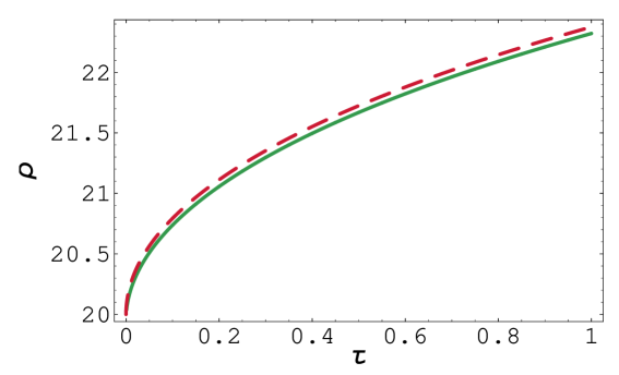
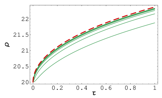
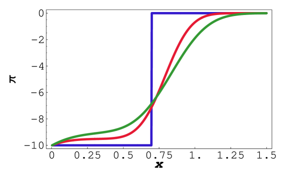
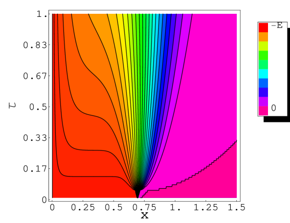
In our first numerical experiment we make attempt to compare our iterative approximation scheme for solving the free boundary problem for an American Call option to known schemes in the case when the volatility is constant. We compare our solution to the one computed by means of a solution to a nonlinear integral equation for as described in Remark 1 (see also [28, 30]). This comparison can be also considered as a benchmark or test example for which we know a solution that can be computed by a another justified algorithm. In Fig. 1, part a), we show the function computed by our iterative algorithm for . At the expiry the value of was computed as: . The corresponding value computed from the integral equation (see [28]) was . The relative error is less than 0.25%. In the part b) we present 7 approximations of the free boundary function computed for different mesh sizes (see Tab. 1 for details). The sequence of approximate free boundaries converges monotonically from below to the free boundary function as . The next part c) of Fig. 1 depicts various solution profiles of a function . In order to achieve a good approximation to equation (28) we need very accurate approximation of for close to the origin . The last part d) of Fig. 1 depicts the contour plot of the function .
In Tab. 1 we present the numerical error analysis for the distance measured in two different norms ( and ) of a computed free boundary position corresponding to the mesh size and the solution computed from the integral equation described in Remark 1 (see also [28]). The time step has been adjusted to the spatial mesh size in order to satisfy CFL condition . We also computed the experimental order of convergence for . Recall that the experimental order of convergence can be defined as the ratio
It can be interpreted as an exponent for which we have . It turns out from Tab. 1 that it is reasonable to make a conjecture that whereas as .
| err() | eoc() | err() | eoc() | |
|---|---|---|---|---|
| 0.03 | 0.5 | - | 0.808 | - |
| 0.012 | 0.215 | 0.92 | 0.227 | 1.39 |
| 0.006 | 0.111 | 0.96 | 0.0836 | 1.44 |
| 0.004 | 0.0747 | 0.97 | 0.0462 | 1.46 |
| 0.003 | 0.0563 | 0.98 | 0.0303 | 1.47 |
| 0.0024 | 0.0452 | 0.98 | 0.0218 | 1.48 |
| 0.002 | 0.0378 | 0.98 | 0.0166 | 1.48 |
4.2 Risk Adjusted Pricing Methodology model
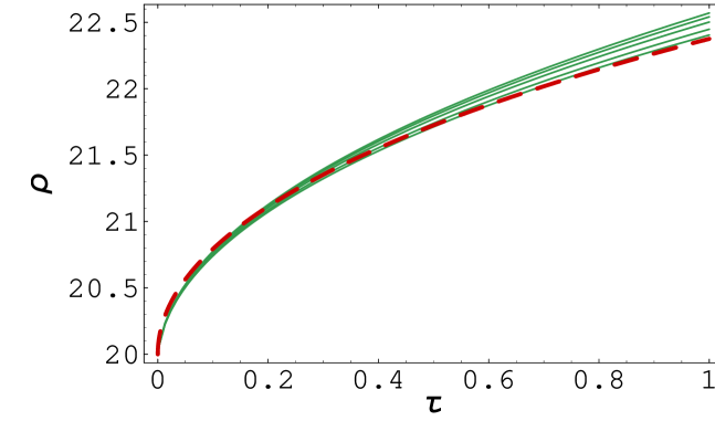
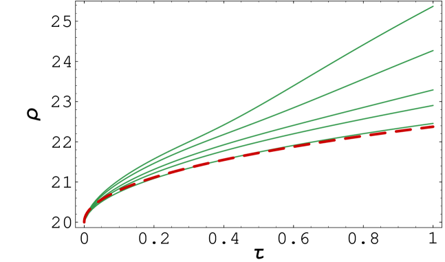
In the next example we computed the position of the free boundary in the case of the Risk Adjusted Pricing Methodology model - a nonlinear Black–Scholes type model derived by Jandačka and Ševčovič in [18]. In this model the volatility is a nonlinear function of the asset price and the second derivative of the option price, and it is given by formula (5). In Fig. 2 we present results of numerical approximation of the free boundary position in the case when the coefficient of transaction costs is fixed and the risk premium measure varies from up to . We compare the position of the free boundary to the case when there are no transaction costs and no risk from volatile portfolio, i.e. we compare it with the free boundary position for the linear Black–Scholes equation (see Fig. 2). An increase in the risk premium coefficient resulted in an increase of the free boundary position as it can be expected.
| 1 | 0.0601 | - | 0.0241 | - |
|---|---|---|---|---|
| 2 | 0.0754 | 0.33 | 0.0303 | 0.328 |
| 5 | 0.102 | 0.33 | 0.0408 | 0.326 |
| 10 | 0.128 | 0.33 | 0.0511 | 0.324 |
| 15 | 0.145 | 0.32 | 0.0582 | 0.323 |
| 20 | 0.16 | 0.32 | 0.0639 | 0.322 |
| 30 | 0.182 | 0.32 | 0.0727 | 0.321 |
| 40 | 0.2 | 0.32 | 0.0798 | 0.32 |
| 50 | 0.214 | 0.32 | 0.0856 | 0.319 |
| 60 | 0.227 | 0.32 | 0.0907 | 0.318 |
| 70 | 0.239 | 0.32 | 0.0953 | 0.317 |
| 80 | 0.249 | 0.32 | 0.0994 | 0.317 |
| 90 | 0.259 | 0.32 | 0.103 | 0.316 |
| 100 | 0.268 | 0.32 | 0.107 | 0.316 |
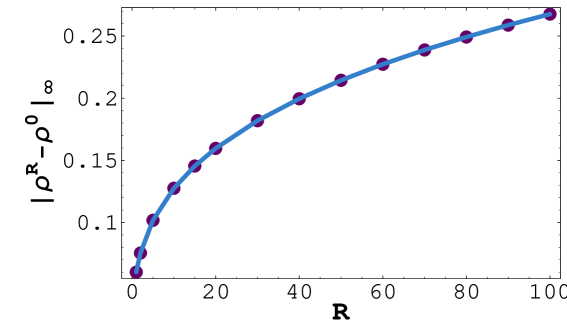
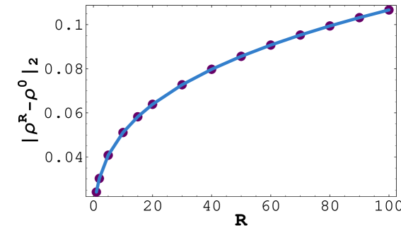
In Tab. 2 and Fig. 2 we summarize results of comparison of the free boundary position for various values of the risk premium coefficient to the reference position computed from the Black–Scholes model with constant volatility , i.e. . The experimental order of the distance function has been computed for , as follows:
According to the values presented in Tab. 2 it turns out that the plausible conjecture is that for both norms and . Since the transaction cost coefficient and risk premium measure enter the expression for the RAPM volatility (5) only in the product we can conjecture that as either or .
4.3 Barles and Soner model
| 0.01 | 0.156 | - | 0.0615 | - |
| 0.02 | 0.25 | 0.68 | 0.0985 | 0.68 |
| 0.05 | 0.472 | 0.69 | 0.184 | 0.679 |
| 0.07 | 0.602 | 0.72 | 0.232 | 0.69 |
| 0.1 | 0.793 | 0.77 | 0.298 | 0.712 |
| 0.11 | 0.857 | 0.82 | 0.32 | 0.74 |
| 0.13 | 0.99 | 0.86 | 0.364 | 0.766 |
| 0.15 | 1.13 | 0.92 | 0.409 | 0.807 |
| 0.2 | 1.52 | 1. | 0.529 | 0.897 |
| 0.25 | 1.97 | 1.2 | 0.669 | 1.05 |
| 0.3 | 2.49 | 1.3 | 0.833 | 1.21 |
| 0.35 | 3.07 | 1.4 | 1.03 | 1.35 |
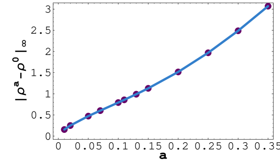
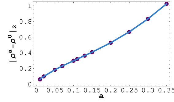
The last example is devoted to the nonlinear Black–Scholes model due to Barles and Soner (see [5]). In this model the volatility is given by equation (3). Numerical results are depicted in Fig. 4. Choosing a larger value of the risk aversion coefficient resulted in increase of the free boundary position . The position of the early exercise boundary has considerably increased in comparison to the linear Black–Scholes equation with constant volatility . In contrast to the case of constant volatility as well as the RAPM model, there is, at least a numerical evidence (see Fig.4 and for the largest ) that the free boundary profile need not be necessarily convex. Recall that that convexity of the free boundary profile has been proved analytically by Ekström et al. and Chen et al. in a recent papers [6, 10, 11] in the case of a American Put option and constant volatility .
Similarly as in the previous model we also investigated the dependence of the free boundary position on the risk aversion parameter . In Tab. 3 and Fig. 5 we present results of comparison of the free boundary position for various values of the risk aversion coefficient to the reference position . Inspecting values of the order of distance it can be conjectured that as . for both norms and .
5 Conclusions
We proposed a new iterative numerical scheme for approximating of the early exercise boundary for a class of Black–Scholes equations for pricing American options with a volatility nonlinearly depending in the asset prices and the second derivative of the option price. The method consisted of transformation the free boundary problem for the early exercise boundary position into a solution of a nonlinear parabolic equation and a nonlinear algebraic constraint equation. The transformed problem has been solved by means of operator splitting iterative technique. We also presented results of numerical approximation of the free boundary for several nonlinear Black–Scholes equation including, in particular, Barles and Soner model and the Risk adjusted pricing methodology model.
References
- [1] Alobaidi, G. (2004) Laplace transforms and installment options. Math. Models & Methods in Appl. Science, 18 (8), 1167–1189.
- [2] Avellaneda, M. & Paras, A. (1994), Dynamic Hedging Portfolios for Derivative Securities in the Presence of Large Transaction Costs. Applied Mathematical Finance, 1, 165–193.
- [3] Barone-Adesi, B. & Whaley, R. E. (1987) Efficient analytic approximations of American option values. J. Finance, 42, 301–320.
- [4] Black, F. & Scholes, M. (1973) The pricing of options and corporate liabilities. J. Political Economy, 81, 637–654.
- [5] Barles, G. & Soner, H. M. (1998) Option Pricing with transaction costs and a nonlinear Black–Scholes equation. Finance Stochast., 2, 369-397.
- [6] Xinfu Chen, Chadam, J., Lishang Jiang, & Weian Zheng (2006) Convexity of the Exercise Boundary of the American Put Option on a Zero Dividend Asset, Mathematical Finance, to appear.
- [7] Dewynne, J. N., Howison, S. D., Rupf, J. & Wilmott, P. (1993) Some mathematical results in the pricing of American options. Euro. J. Appl. Math., 4, 381–398.
- [8] During, B., Fournier, M. & Jungel, A. (2003) High order compact finite difference schemes for a nonlinear Black–Scholes equation. Int. J. Appl. Theor. Finance, 7, 767–789.
- [9] Ehrhardt, M. & Mickens, R. (2006) Discrete artificial boundary conditions for the Black–Scholes equation of American options, submmitted.
- [10] Ekström, E. & Tysk, J. (2006) The American put is log-concave in the log-price. Journal of Mathematical Analysis and Appl., 314(2), 710–723.
- [11] Ekström, E. (2004) Convexity of the optimal stopping boundary for the American put option Journal of Mathematical Analysis and Appl., 299(1), 147–156.
- [12] Frey, R. & Patie, P. (2002) Risk Management for Derivatives in Illiquid Markets: A Simulation Study. Advances in Finance and Stochastics, Springer, Berlin, 137–159.
- [13] Frey, R. & Stremme, A. (1997) Market Volatility and Feedback Effects from Dynamic Hedging. Mathematical Finance, 4, 351–374.
- [14] Geske, R. & Johnson, H. E. (1984) The American put option valued analytically. J. Finance, 39, 1511–1524.
- [15] Geske, R. & Roll, R. (1984) On valuing American call options with the Black–Scholes European formula. J. Finance, 89, 443–455.
- [16] Hull, J. (1989) Options, Futures and Other Derivative Securities, Prentice Hall.
- [17] Hoggard, T., Whalley, A.E. & Wilmott, P. (1994) Hedging option portfolios in the presence of transaction costs. Advances in Futures and Options Research, 7, 21–35.
- [18] Jandačka, M., & Ševčovič, D. (2005) On the risk adjusted pricing methodology based valuation of vanilla options and explanation of the volatility smile. Journal of Applied Mathematics, 3, 235–258.
- [19] Kuske R. A. & Keller, J. B. (1998) Optimal exercise boundary for an American put option. Applied Mathematical Finance, 5, 107–116.
- [20] Kratka, M. (1998) No Mystery Behind the Smile, Risk, 9, 67–71.
- [21] Kwok, Y. K. (1998) Mathematical Models of Financial Derivatives. Springer-Verlag.
- [22] Leland, H. E. (1985) Option pricing and replication with transaction costs Journal of Finance, 40, 1283–1301.
- [23] MacMillan, L. W. (1986) Analytic approximation for the American put option. Adv. in Futures Options Res., 1, 119–134.
- [24] Mallier, R. (2002) Evaluating approximations for the American put option. Journal of Applied Mathematics, 2, 71–92.
- [25] Mallier, R. & Alobaidi, G. (2004) The American put option close to expiry. Acta Mathematica Univ. Comenianae, 73, 161–174.
- [26] Mynemi, R. (1992) The pricing of the American option. Annal. Appl. Probab., 2, 1–23.
- [27] Roll, R. (1977) An analytic valuation formula for unprotected American call options on stock with known dividends. J. Finan. Economy, 5, 251–258.
- [28] Ševčovič, D. (2001) Analysis of the free boundary for the pricing of an American call option. Euro. Journal on Applied Mathematics, 12, 25–37.
- [29] Schönbucher, P., & Wilmott, P. (2000) The feedback-effect of hedging in illiquid markets. SIAM Journal of Applied Mathematics, 61, 232–272.
- [30] Stamicar, R., Ševčovič, D. & Chadam, J. (1999) The early exercise boundary for the American put near expiry: numerical approximation. Canad. Appl. Math. Quarterly, 7, 427–444.
- [31] Jichao Zhao, Corless, R. M., & Davison, M. (2005) Compact finite difference method for American option pricing. Journal of Computational and Applied Mathematics, to appear, available online 22 August 2006.