This paper was converted on www.awesomepapers.org from LaTeX by an anonymous user.
Want to know more? Visit the Converter page.

An Iterative Algorithm for Regularized Non-negative Matrix Factorizations

Steven E. Pav steven@gilgamath.com Application of the multiplicative methods described herein for chemometrics applications may be covered by U.S. Patent. [7]
Abstract

We generalize the non-negative matrix factorization algorithm of Lee and Seung [3] to accept a weighted norm, and to support ridge and Lasso regularization. We recast the Lee and Seung multiplicative update as an additive update which does not get stuck on zero values. We apply the companion R package rnnmf [9] to the problem of finding a reduced rank representation of a database of cocktails.

1 Introduction

The term non-negative matrix factorization refers to decomposing a given matrix 𝖸\mathsf{Y} with non-negative elements approximately as the product 𝖸𝖫𝖱\mathsf{Y}\approx\mathsf{L}\mathsf{R}, for comformable non-negative matrices 𝖫\mathsf{L} and 𝖱\mathsf{R} of smaller rank than 𝖸\mathsf{Y}. This factorization represents a kind of dimensionality reduction. The quality of the approximation is measured by some “divergence” between 𝖸\mathsf{Y} and 𝖫𝖱\mathsf{L}\mathsf{R}, or some norm of their difference. Perhaps the most common is the Frobenius (or elementwise 2\ell_{2}) distance between them. Under this objective, non-negative matrix factorization can be expressed as the optimization problem:

min𝖫0,𝖱0tr((𝖸𝖫𝖱)(𝖸𝖫𝖱)),\min_{\mathsf{L}\geq 0,\,\mathsf{R}\geq 0}\operatorname{tr}\left({{\left(\mathsf{Y}-\mathsf{L}\mathsf{R}\right)}^{\top}}\left(\mathsf{Y}-\mathsf{L}\mathsf{R}\right)\right), (1)

where tr(𝖬)\operatorname{tr}\left(\mathsf{M}\right) is the trace of the matrix 𝖬\mathsf{M}, and 𝖠0\mathsf{A}\geq 0 means the elements of 𝖠\mathsf{A} are non-negative. [10]

Lee and Seung described an iterative approach to this problem, as well as for a related optimization with a different objective. [3] Their algorithm starts with some unspecified initial iterates 𝖫(0){\mathsf{L}}^{\left(0\right)} and 𝖱(0){\mathsf{R}}^{\left(0\right)}, then iteratively improves 𝖫(k){\mathsf{L}}^{\left(k\right)} and 𝖱(k){\mathsf{R}}^{\left(k\right)} in turn. That is, given 𝖫(k){\mathsf{L}}^{\left(k\right)} and 𝖱(k){\mathsf{R}}^{\left(k\right)}, an update is made to arrive at 𝖫(k+1){\mathsf{L}}^{\left(k+1\right)}; then using 𝖫(k+1){\mathsf{L}}^{\left(k+1\right)} and 𝖱(k){\mathsf{R}}^{\left(k\right)}, one computes 𝖱(k+1){\mathsf{R}}^{\left(k+1\right)}, and the process repeats. The iterative update for 𝖫(k+1){\mathsf{L}}^{\left(k+1\right)} is

𝖫(k+1)𝖫(k)𝖸𝖱(k)(𝖫(k)𝖱(k)𝖱(k)).{\mathsf{L}}^{\left(k+1\right)}\leftarrow{\mathsf{L}}^{\left(k\right)}\odot\mathsf{Y}{{{\mathsf{R}}^{\left(k\right)}}^{\top}}\mathit{\oslash}\left({\mathsf{L}}^{\left(k\right)}{\mathsf{R}}^{\left(k\right)}{{{\mathsf{R}}^{\left(k\right)}}^{\top}}\right). (2)

We use \odot to mean the Hadamard, or ‘elementwise’, multiplication, and \mathit{\oslash} to mean Hadamard division. The iterative update for 𝖱(k+1){\mathsf{R}}^{\left(k+1\right)} is defined mutatis mutandis. As should be apparent from inspection, this iterative update maintains non-negativity of estimates. That is, if 𝖸\mathsf{Y}, 𝖫(k){\mathsf{L}}^{\left(k\right)}, and 𝖱(k){\mathsf{R}}^{\left(k\right)} have only positive elements, then 𝖫(k+1){\mathsf{L}}^{\left(k+1\right)} is finite and has only positive elements. It is not clear what should be done if elements of the denominator term 𝖫(k){\mathsf{L}}^{\left(k\right)} 𝖱(k)𝖱(k){\mathsf{R}}^{\left(k\right)}{{{\mathsf{R}}^{\left(k\right)}}^{\top}} are zero, and whether and how this can be avoided.

Gonzalez and Zhang describe a modification of the update to accelerate convergence. [2] Their accelerated algorithm updates 𝖫(k){\mathsf{L}}^{\left(k\right)} row by row, and 𝖱(k){\mathsf{R}}^{\left(k\right)} column by column, using the step length modification of Merritt and Zhang [5].

One attractive feature of the Lee and Seung iterative update is its sheer simplicity. In a high-level computer language with a rich set of matrix operations, such as Julia or octave, the iterative step can be expressed in a single line of code; the entire algorithm could be expressed in perhaps 20 lines of code. Conceivably this algorithm could even be implemented in challenged computing environments, like within a SQL query or a spreadsheet macro language. Simplicity makes this algorithm an obvious choice for experimentation without requiring an all-purpose constrained quadratic optimization solver, or other complicated software.

2 Regularized Non-Negative Matrix Factorization

We generalize the optimization problem of 1 to include a weighted norm, regularization terms, and orthogonality penalties. For a given 𝖸\mathsf{Y}, and non-negative weighting matrices 𝖶0,R{\mathsf{W}}_{0,R}, 𝖶0,C{\mathsf{W}}_{0,C}, 𝖶1,L{\mathsf{W}}_{1,L}, 𝖶1,R{\mathsf{W}}_{1,R}, 𝖶2,R,L,j{\mathsf{W}}_{2,R,L,j}, 𝖶2,C,L,j{\mathsf{W}}_{2,C,L,j}, 𝖶2,R,R,j{\mathsf{W}}_{2,R,R,j}, and 𝖶2,C,R,j{\mathsf{W}}_{2,C,R,j}, find matrices 𝖫\mathsf{L} and 𝖱\mathsf{R} to minimize

min𝖫0,𝖱0\displaystyle\min_{\mathsf{L}\geq 0,\,\mathsf{R}\geq 0}\,\, 12tr((𝖸𝖫𝖱)𝖶0,R(𝖸𝖫𝖱)𝖶0,C)\displaystyle\frac{1}{2}\operatorname{tr}\left({{\left(\mathsf{Y}-\mathsf{L}\mathsf{R}\right)}^{\top}}{\mathsf{W}}_{0,R}\left(\mathsf{Y}-\mathsf{L}\mathsf{R}\right){\mathsf{W}}_{0,C}\right) (3)
+tr(𝖶1,L𝖫)+tr(𝖶1,R𝖱)\displaystyle\phantom{=}\,+\operatorname{tr}\left({{{\mathsf{W}}_{1,L}}^{\top}}\mathsf{L}\right)+\operatorname{tr}\left({{{\mathsf{W}}_{1,R}}^{\top}}\mathsf{R}\right)
+121jJtr(𝖫𝖶2,R,L,j𝖫𝖶2,C,L,j)\displaystyle\phantom{=}\,+\frac{1}{2}\sum_{1\leq j\leq J}\operatorname{tr}\left({{\mathsf{L}}^{\top}}{\mathsf{W}}_{2,R,L,j}\mathsf{L}{\mathsf{W}}_{2,C,L,j}\right)
+121jJtr(𝖱𝖶2,R,R,j𝖱𝖶2,C,R,j).\displaystyle\phantom{=}\,+\frac{1}{2}\sum_{1\leq j\leq J}\operatorname{tr}\left({{\mathsf{R}}^{\top}}{\mathsf{W}}_{2,R,R,j}\mathsf{R}{\mathsf{W}}_{2,C,R,j}\right).

Essentially we are trying to model 𝖸\mathsf{Y} as 𝖫𝖱\mathsf{L}\mathsf{R}. Our loss function is quadratic in the error 𝖸𝖫𝖱\mathsf{Y}-\mathsf{L}\mathsf{R}, with weights 𝖶0,R{\mathsf{W}}_{0,R} and 𝖶0,C{\mathsf{W}}_{0,C}, and 1\ell_{1} and 2\ell_{2} regularization via the terms with 𝖶1{\mathsf{W}}_{1} and 𝖶2,R,j{\mathsf{W}}_{2,R,j} and 𝖶2,C,j{\mathsf{W}}_{2,C,j}. This optimization problem includes that of 1 as a special case.

We note that a non-orthogonality penalty term on the 𝖷\mathsf{X} can be expressed as

c2tr(𝖷𝖨𝖷(𝟏𝟏𝖨)).\frac{c}{2}\operatorname{tr}\left({{\mathsf{X}}^{\top}}\mathsf{I}\mathsf{X}\left(\boldsymbol{1}{{\boldsymbol{1}}^{\top}}-\mathsf{I}\right)\right).

Thus a non-orthogonality penalty term can be expressed with the 𝖶2,R,j{\mathsf{W}}_{2,R,j} and 𝖶2,C,j{\mathsf{W}}_{2,C,j}. Indeed the motivation for including a sum of the 2\ell_{2} terms is to allow for both straightforward regularization, where 𝖶2,R,j=𝖨{\mathsf{W}}_{2,R,j}=\mathsf{I} and 𝖶2,C,j=c𝖨{\mathsf{W}}_{2,C,j}=c\mathsf{I}, and orthogonality terms. For simplicity of notation, in the discussion that follows we will often treat the 2\ell_{2} terms as if there were only one of them, i.e., J=1J=1, and omit the jj subscripts. Restoring the more general case consists only of expanding to a full sum of JJ terms.

This problem formulation is appropriate for power users who can meaningfully select the various weighting matrices. And while it is easy to conceive of a use for general forms for 𝖶0,R{\mathsf{W}}_{0,R} and 𝖶0,C{\mathsf{W}}_{0,C} (the rows of 𝖸\mathsf{Y} have different importances, or the columns of 𝖸\mathsf{Y} are observed with different accuracies, for example), most users would probably prefer simpler formulations for the 𝖶1,{\mathsf{W}}_{1,\cdot} and 𝖶2,,,j{\mathsf{W}}_{2,\cdot,\cdot,j} matrices. To achieve something like an elasticnet factorization with non-orthogonality penalties, one should set J=2J=2 and take

𝖶1,L\displaystyle{\mathsf{W}}_{1,L} =λ1,L𝟣,\displaystyle=\lambda_{1,L}\mathsf{1}, 𝖶1,R\displaystyle\quad{\mathsf{W}}_{1,R} =λ1,R𝟣,\displaystyle=\lambda_{1,R}\mathsf{1},
𝖶2,R,L,1\displaystyle{\mathsf{W}}_{2,R,L,1} =λ2,L𝖨,\displaystyle=\lambda_{2,L}\mathsf{I}, 𝖶2,C,L,1\displaystyle\quad{\mathsf{W}}_{2,C,L,1} =𝖨,\displaystyle=\mathsf{I},
𝖶2,R,R,1\displaystyle{\mathsf{W}}_{2,R,R,1} =λ2,R𝖨,\displaystyle=\lambda_{2,R}\mathsf{I}, 𝖶2,C,R,1\displaystyle\quad{\mathsf{W}}_{2,C,R,1} =𝖨,\displaystyle=\mathsf{I}, (4)
𝖶2,R,L,2\displaystyle{\mathsf{W}}_{2,R,L,2} =𝖨,\displaystyle=\mathsf{I}, 𝖶2,C,L,2\displaystyle\quad{\mathsf{W}}_{2,C,L,2} =γ2,L(𝟏𝟏𝖨),\displaystyle=\gamma_{2,L}\left(\boldsymbol{1}{{\boldsymbol{1}}^{\top}}-\mathsf{I}\right),
𝖶2,R,R,2\displaystyle{\mathsf{W}}_{2,R,R,2} =𝖨,\displaystyle=\mathsf{I}, 𝖶2,C,R,2\displaystyle\quad{\mathsf{W}}_{2,C,R,2} =γ2,R(𝟏𝟏𝖨),\displaystyle=\gamma_{2,R}\left(\boldsymbol{1}{{\boldsymbol{1}}^{\top}}-\mathsf{I}\right),

where here 𝟣\mathsf{1} stands in for an all-ones matrix of the appropriate size. All the λ\lambda and γ\gamma parameters must be non-negative, and the identity matrices are all appropriately sized. This is the reduced form of the problem that depends mostly on a few scalars. A simple form for the weighted error is to take 𝖶0,R{\mathsf{W}}_{0,R} and 𝖶0,C{\mathsf{W}}_{0,C} to be diagonal matrices,

Depending on the regularization terms, the solution to the problem of 3 is unlikely to be unique. Certain the solution to 1 is not unique, since if 𝖰\mathsf{Q} is a permutation matrix of the appropriate size, then 𝖫𝖰\mathsf{L}\mathsf{Q} and 𝖰1𝖱{{\mathsf{Q}}^{-1}}\mathsf{R} are another set of non-negative matrices with the same objective value. Perhaps the regularization terms can help avoid these kinds of ambiguity in the solution.

2.0.1 Split Form

To approximately solve this problem our algorithm starts with some initial estimates of 𝖫\mathsf{L} and 𝖱\mathsf{R} and iteratively alternates between updating the estimate of 𝖫\mathsf{L} with the estimate of 𝖱\mathsf{R} fixed, and updating the estimate of 𝖱\mathsf{R} with the estimate of 𝖫\mathsf{L} fixed. To discuss these half-step updates, we can describe both of them in a single unified formulation. So we consider the optimization problem

min𝖷0ϕ(𝖷),\min_{\mathsf{X}\geq 0}\phi\left(\mathsf{X}\right), (5)

where we define the objective function

ϕ(𝖷)\displaystyle\phi\left(\mathsf{X}\right) =12tr((𝖸𝖫𝖷𝖱)𝖶0,R(𝖸𝖫𝖷𝖱)𝖶0,C)\displaystyle=\frac{1}{2}\operatorname{tr}\left({{\left(\mathsf{Y}-\mathsf{L}\mathsf{X}\mathsf{R}\right)}^{\top}}{\mathsf{W}}_{0,R}\left(\mathsf{Y}-\mathsf{L}\mathsf{X}\mathsf{R}\right){\mathsf{W}}_{0,C}\right) (6)
+tr(𝖶1𝖷)+121jJtr(𝖷𝖶2,R,j𝖷𝖶2,C,j).\displaystyle\phantom{=}\,+\operatorname{tr}\left({{{\mathsf{W}}_{1}}^{\top}}\mathsf{X}\right)+\frac{1}{2}\sum_{1\leq j\leq J}\operatorname{tr}\left({{\mathsf{X}}^{\top}}{\mathsf{W}}_{2,R,j}\mathsf{X}{\mathsf{W}}_{2,C,j}\right).

We must assume that 𝖫\mathsf{L} has full column rank and 𝖱\mathsf{R} has full row rank, 𝖶0,R{\mathsf{W}}_{0,R}, 𝖶0,C{\mathsf{W}}_{0,C}, 𝖶2,R,j{\mathsf{W}}_{2,R,j} and 𝖶2,C,j{\mathsf{W}}_{2,C,j} are square, symmetric and positive semidefinite. The 𝖶0,R{\mathsf{W}}_{0,R} has the same number of rows as 𝖸\mathsf{Y}, and 𝖶0,C{\mathsf{W}}_{0,C} has the same number of columns as 𝖸\mathsf{Y}. 𝖶1{\mathsf{W}}_{1} is the same size as 𝖷\mathsf{X}; we will make further restrictions on 𝖶1{\mathsf{W}}_{1} below. The matrices 𝖶2,R,j{\mathsf{W}}_{2,R,j} have the same number of rows as 𝖷\mathsf{X}, and 𝖶2,C,j{\mathsf{W}}_{2,C,j} have the same number of columns as 𝖷\mathsf{X}. All the 𝖶i,{\mathsf{W}}_{i,\cdot} are assumed to have non-negative elements, that is 𝖶i,0{\mathsf{W}}_{i,\cdot}\geq 0.

Our algorithm now consists of filling in an identity for 𝖫\mathsf{L}, and estimate of 𝖫\mathsf{L} for 𝖷\mathsf{X}, and all the 𝖫\mathsf{L}-appropriate weighting matrices into Equation 6 and taking a step to solve Problem 3, getting an update of 𝖫\mathsf{L}. Then we perform a similar operation to get a new estimate of 𝖱\mathsf{R}.

2.1 Factorization in Vector Form

The analysis is simplified if we express the problem as one of finding a vector unknown, so we will ‘vectorize’ the problem. For matrix 𝖬\mathsf{M} let vec(𝖬)\operatorname{vec}\left(\mathsf{M}\right) be the vector which consists of the columns of 𝖬\mathsf{M} stacked on top of each other; let 𝖠𝖡{\mathsf{A}}\otimes{\mathsf{B}} denote the Kronecker product of 𝖠\mathsf{A} and 𝖡\mathsf{B}. [11] See Section A in the appendix for some helpful identities involving the Kronecker product, matrix trace, and vectorization.

We write ϕ(𝖷)\phi\left(\mathsf{X}\right) as a quadratic function of the vector vec(𝖷)\operatorname{vec}\left(\mathsf{X}\right)

ϕ(𝖷)=12vec(𝖸)(𝖱𝖫)vec(𝖷)𝖶0,C𝖶0,R2+12jvec(𝖷)𝖶2,C,j𝖶2,R,j2+vec(𝖶1)vec(𝖷)=12vec(𝖷)𝖦vec(𝖷)+𝒅vec(𝖷)+c,\begin{split}\phi\left(\mathsf{X}\right)&=\frac{1}{2}\left\|{\operatorname{vec}\left(\mathsf{Y}\right)-\left({{{\mathsf{R}}^{\top}}}\otimes{\mathsf{L}}\right)\operatorname{vec}\left(\mathsf{X}\right)}\right\|_{{{\mathsf{W}}_{0,C}}\otimes{{\mathsf{W}}_{0,R}}}^{2}\\ &+\frac{1}{2}\sum_{j}\left\|{\operatorname{vec}\left(\mathsf{X}\right)}\right\|_{{{\mathsf{W}}_{2,C,j}}\otimes{{\mathsf{W}}_{2,R,j}}}^{2}+{{\operatorname{vec}\left({\mathsf{W}}_{1}\right)}^{\top}}\operatorname{vec}\left(\mathsf{X}\right)\\ &=\frac{1}{2}{{\operatorname{vec}\left(\mathsf{X}\right)}^{\top}}\mathsf{G}\operatorname{vec}\left(\mathsf{X}\right)+{{\boldsymbol{d}}^{\top}}\operatorname{vec}\left(\mathsf{X}\right)+c,\end{split} (7)

where

𝖦=(𝖱𝖫)(𝖶0,C𝖶0,R)(𝖱𝖫)+j𝖶2,C,j𝖶2,R,j,=(𝖱𝖶0,C𝖱)(𝖫𝖶0,R𝖫)+j𝖶2,C,j𝖶2,R,j.𝒅=vec(𝖶1)(𝖱𝖫)(𝖶0,C𝖶0,R)vec(𝖸),=vec(𝖶1)vec(𝖫𝖶0,R𝖸𝖶0,C𝖱).\begin{split}\mathsf{G}&={{\left({{{\mathsf{R}}^{\top}}}\otimes{\mathsf{L}}\right)}^{\top}}\left({{\mathsf{W}}_{0,C}}\otimes{{\mathsf{W}}_{0,R}}\right)\left({{{\mathsf{R}}^{\top}}}\otimes{\mathsf{L}}\right)+\sum_{j}{{\mathsf{W}}_{2,C,j}}\otimes{{\mathsf{W}}_{2,R,j}},\\ &=\left(\mathsf{R}{\mathsf{W}}_{0,C}{{\mathsf{R}}^{\top}}\right)\otimes\left({{\mathsf{L}}^{\top}}{\mathsf{W}}_{0,R}\mathsf{L}\right)+\sum_{j}{{\mathsf{W}}_{2,C,j}}\otimes{{\mathsf{W}}_{2,R,j}}.\\ \boldsymbol{d}&={\operatorname{vec}\left({\mathsf{W}}_{1}\right)}-{{\left({{{\mathsf{R}}^{\top}}}\otimes{\mathsf{L}}\right)}^{\top}}\left({{\mathsf{W}}_{0,C}}\otimes{{\mathsf{W}}_{0,R}}\right)\operatorname{vec}\left(\mathsf{Y}\right),\\ &={\operatorname{vec}\left({\mathsf{W}}_{1}\right)}-\operatorname{vec}\left({{\mathsf{L}}^{\top}}{\mathsf{W}}_{0,R}\mathsf{Y}{\mathsf{W}}_{0,C}{{\mathsf{R}}^{\top}}\right).\end{split} (8)

We write 𝒙𝖠2\left\|{\boldsymbol{x}}\right\|_{\mathsf{A}}^{2} to mean 𝒙𝖠𝒙{{\boldsymbol{x}}^{\top}}\mathsf{A}\boldsymbol{x}. Note that 𝖦0\mathsf{G}\geq 0, but 𝒅\boldsymbol{d} will likely have negative elements. In fact, to use Lee and Seung’s iterative algorithm, the vector 𝒅\boldsymbol{d} must have non-positive elements. This is equivalent to the restriction 𝖫𝖶0,R𝖸𝖶0,C𝖱𝖶10{{\mathsf{L}}^{\top}}{{\mathsf{W}}_{0,R}}\mathsf{Y}{\mathsf{W}}_{0,C}\mathsf{R}-{\mathsf{W}}_{1}\geq 0, taken elementwise. This imposes a restriction on 𝖶1{\mathsf{W}}_{1} which is hard to verify for the problem of non-negative matrix factorization. Note that by definition 𝖦\mathsf{G} can be positive definite, depending on the 𝖱\mathsf{R}, 𝖫\mathsf{L} and the 𝖶2,{\mathsf{W}}_{2,\cdot}, but is only positive semi definite in the general case.

We can thus consider this problem as optimization over a vector unknown. In an abuse of notation, we reuse the objective function ϕ()\phi\left(\cdot\right), writing

ϕ(𝒙)=12𝒙𝖦𝒙+𝒅𝒙,\phi\left({\boldsymbol{x}}\right)=\frac{1}{2}{{{\boldsymbol{x}}}^{\top}}\mathsf{G}{\boldsymbol{x}}+{{\boldsymbol{d}}^{\top}}{\boldsymbol{x}}, (9)

for symmetric, nonnegative positive semidefinite 𝖦\mathsf{G}. So now we consider the positivity-constrained quadratic optimization problem

min𝒙0ϕ(𝒙).\min_{{\boldsymbol{x}}\geq 0}\phi\left({\boldsymbol{x}}\right). (10)

Note that the unconstrained solution to this problem is 𝖦1𝒅-{{\mathsf{G}}^{-1}}{\boldsymbol{d}}. When 𝖦\mathsf{G} is positive definite, because the constraint space is convex, this solution will be unique. [6] In general, however, we will not have unique solutions. When the 𝖶1{\mathsf{W}}_{1} term is all zero, this a weighted least squares problem, possibly with Tikhonov regularization.

The gradient of the objective ϕ(𝒙)\phi\left({\boldsymbol{x}}\right) is is ϕ(𝒙)=𝖦𝒙+𝒅\nabla\phi\left({\boldsymbol{x}}\right)=\mathsf{G}{\boldsymbol{x}}+\boldsymbol{d}. When considering the matrix form of the problem, this has the value

vec([𝖫𝖶0,R𝖫𝖷𝖱𝖶0,C𝖱+j𝖶2,R,j𝖷𝖶2,C,j+𝖶1𝖫𝖶0,R𝖸𝖶0,C𝖱]).\operatorname{vec}\left(\left[{{\mathsf{L}}^{\top}}{\mathsf{W}}_{0,R}\mathsf{L}\mathsf{X}\mathsf{R}{\mathsf{W}}_{0,C}{{\mathsf{R}}^{\top}}+\sum_{j}{\mathsf{W}}_{2,R,j}\mathsf{X}{\mathsf{W}}_{2,C,j}+{\mathsf{W}}_{1}-{{\mathsf{L}}^{\top}}{\mathsf{W}}_{0,R}\mathsf{Y}{\mathsf{W}}_{0,C}{{\mathsf{R}}^{\top}}\right]\right).

We consider an iterative solution to this problem. We first select some 𝒙(0){\boldsymbol{x}}^{\left(0\right)}. Then given current iterate 𝒙(k){\boldsymbol{x}}^{\left(k\right)}, we seek to find the next iterate 𝒙(k+1){\boldsymbol{x}}^{\left(k+1\right)}. Define

ϕ(k)(𝒙)=12𝒙𝖦(k)𝒙+𝒅(k)𝒙+ck,{\phi}^{\left(k\right)}\left({\boldsymbol{x}}\right)=\frac{1}{2}{{{\boldsymbol{x}}}^{\top}}{\mathsf{G}}^{\left(k\right)}{\boldsymbol{x}}+{{{\boldsymbol{d}}^{\left(k\right)}}^{\top}}{\boldsymbol{x}}+c_{k},

where we will set 𝖦(k){\mathsf{G}}^{\left(k\right)}, 𝒅(k){\boldsymbol{d}}^{\left(k\right)} and ckc_{k} such that ϕ(k)(𝒙){\phi}^{\left(k\right)}\left({\boldsymbol{x}}\right) is tangent to ϕ(𝒙)\phi\left({\boldsymbol{x}}\right) at 𝒙(k){\boldsymbol{x}}^{\left(k\right)}, and such that ϕ(k)(𝒙)ϕ(𝒙){\phi}^{\left(k\right)}\left({\boldsymbol{x}}\right)\geq\phi\left({\boldsymbol{x}}\right) for all 𝒙{\boldsymbol{x}}. We will take 𝒙(k+1){\boldsymbol{x}}^{\left(k+1\right)} as some point which improves ϕ(k)(𝒙){\phi}^{\left(k\right)}\left({\boldsymbol{x}}\right): its minimizer if it is non-negative, or another point if not. If 𝒙(k+1){\boldsymbol{x}}^{\left(k+1\right)} improves ϕ(k)(𝒙){\phi}^{\left(k\right)}\left({\boldsymbol{x}}\right), then it also improves ϕ(𝒙)\phi\left({\boldsymbol{x}}\right), as

ϕ(𝒙(k+1))ϕ(k)(𝒙(k+1))ϕ(k)(𝒙(k))=ϕ(𝒙(k)).\phi\left({\boldsymbol{x}}^{\left(k+1\right)}\right)\leq{\phi}^{\left(k\right)}\left({\boldsymbol{x}}^{\left(k+1\right)}\right)\leq{\phi}^{\left(k\right)}\left({\boldsymbol{x}}^{\left(k\right)}\right)=\phi\left({\boldsymbol{x}}^{\left(k\right)}\right).

The tangency condition fixes the value of ckc_{k}, and also gives the identity

𝒅(k)=𝒅+𝖦𝒙(k)𝖦(k)𝒙(k).{\boldsymbol{d}}^{\left(k\right)}={\boldsymbol{d}}+\mathsf{G}{\boldsymbol{x}}^{\left(k\right)}-{\mathsf{G}}^{\left(k\right)}{\boldsymbol{x}}^{\left(k\right)}.

To ensure that ϕ(k)(𝒙)ϕ(𝒙){\phi}^{\left(k\right)}\left({\boldsymbol{x}}\right)\geq\phi\left({\boldsymbol{x}}\right) it is sufficient to select select 𝖦(k){\mathsf{G}}^{\left(k\right)} such that 𝖦(k)𝖦{\mathsf{G}}^{\left(k\right)}-\mathsf{G} is positive semidefinite. The following lemma gives us a way of selecting diagonal matrices 𝖦(k){\mathsf{G}}^{\left(k\right)} that satisfy this condition.

First a bit of notation, for vector 𝒗\boldsymbol{v}, Diag(𝒗)\operatorname{Diag}\left(\boldsymbol{v}\right) is the diagonal matrix with 𝒗\boldsymbol{v} for diagonal. For matrix 𝖠\mathsf{A}, diag(𝖠)\operatorname{diag}\left(\mathsf{A}\right) is the vector of the diagonal of 𝖠\mathsf{A}. Thus we have diag(Diag(𝒗))=𝒗\operatorname{diag}\left(\operatorname{Diag}\left(\boldsymbol{v}\right)\right)=\boldsymbol{v}.

Lemma 2.1.

Let 𝖦\mathsf{G} be a symmetric matrix with non-negative elements, and full rank, and let 𝐛\boldsymbol{b} be a vector with strictly positive elements. Then

Diag(𝖦𝒃)Diag(𝒃)1𝖦.\operatorname{Diag}\left(\mathsf{G}\boldsymbol{b}\right){{\operatorname{Diag}\left(\boldsymbol{b}\right)}^{-1}}\succeq\mathsf{G}.

(Here 𝖠𝖡\mathsf{A}\succeq\mathsf{B} means that 𝖠𝖡\mathsf{A}-\mathsf{B} is positive semidefinite.)

Proof.

First note that if 𝖠\mathsf{A} is symmetric, and has non-negative elements, then Diag(𝖠𝟏)𝖠\operatorname{Diag}\left(\mathsf{A}\boldsymbol{1}\right)\succeq\mathsf{A} because the matrix Diag(𝖠𝟏)𝖠\operatorname{Diag}\left(\mathsf{A}\boldsymbol{1}\right)-\mathsf{A} is symmetric, with non-negative diagonal, and is diagonally dominant, thus it is positive semidefinite.

Apply that fact with 𝖠=Diag(𝒃)𝖦Diag(𝒃)\mathsf{A}=\operatorname{Diag}\left(\boldsymbol{b}\right)\mathsf{G}\operatorname{Diag}\left(\boldsymbol{b}\right). Then

Diag(Diag(𝒃)𝖦Diag(𝒃)𝟏)\displaystyle\operatorname{Diag}\left(\operatorname{Diag}\left(\boldsymbol{b}\right)\mathsf{G}\operatorname{Diag}\left(\boldsymbol{b}\right)\boldsymbol{1}\right) Diag(𝒃)𝖦Diag(𝒃),\displaystyle\succeq\operatorname{Diag}\left(\boldsymbol{b}\right)\mathsf{G}\operatorname{Diag}\left(\boldsymbol{b}\right),
Diag(𝒃)Diag(𝖦𝒃)\displaystyle\operatorname{Diag}\left(\boldsymbol{b}\right)\operatorname{Diag}\left(\mathsf{G}\boldsymbol{b}\right) Diag(𝒃)𝖦Diag(𝒃),\displaystyle\succeq\operatorname{Diag}\left(\boldsymbol{b}\right)\mathsf{G}\operatorname{Diag}\left(\boldsymbol{b}\right),
Diag(𝖦𝒃)Diag(𝒃)1\displaystyle\operatorname{Diag}\left(\mathsf{G}\boldsymbol{b}\right){{\operatorname{Diag}\left(\boldsymbol{b}\right)}^{-1}} 𝖦,\displaystyle\succeq\mathsf{G},

as needed.

Note that the proof relies on strict positivity of the elements of 𝒃\boldsymbol{b}. By this we can claim a bijection between n\mathbb{R}^{n} and Diag(𝒃)n\operatorname{Diag}\left(\boldsymbol{b}\right)\mathbb{R}^{n}, which allows us to conclude the last line above. ∎

Lemma 2.2.

Let 𝖦\mathsf{G} be a symmetric matrix with non-negative elements, and full rank. Let 𝐛\boldsymbol{b} be some vector with non-negative elements such that 𝖦𝐛\mathsf{G}\boldsymbol{b} has strictly positive elements. Letting

𝒙(k+1)𝒙(k)Diag(𝒃)Diag(𝖦𝒃)1(𝒅+𝖦𝒙(k)),{\boldsymbol{x}}^{\left(k+1\right)}\leftarrow{\boldsymbol{x}}^{\left(k\right)}-\operatorname{Diag}\left(\boldsymbol{b}\right){{\operatorname{Diag}\left(\mathsf{G}\boldsymbol{b}\right)}^{-1}}\left({\boldsymbol{d}}+\mathsf{G}{\boldsymbol{x}}^{\left(k\right)}\right),

then ϕ(𝐱(k+1))ϕ(𝐱(k)).\phi\left({\boldsymbol{x}}^{\left(k+1\right)}\right)\leq\phi\left({\boldsymbol{x}}^{\left(k\right)}\right).

Proof.

First, consider the case where 𝒃\boldsymbol{b} has strictly positive elements. Letting 𝖦(k)=Diag(𝖦𝒃)Diag(𝒃)1,{\mathsf{G}}^{\left(k\right)}=\operatorname{Diag}\left(\mathsf{G}\boldsymbol{b}\right){{\operatorname{Diag}\left(\boldsymbol{b}\right)}^{-1}}, the minimum of ϕ(k)(𝒙){\phi}^{\left(k\right)}\left({\boldsymbol{x}}\right) occurs at 𝖦(k)1𝒅(k)-{{{\mathsf{G}}^{\left(k\right)}}^{-1}}{\boldsymbol{d}}^{\left(k\right)}, which has value

𝖦(k)1𝒅(k)=𝖦(k)1(𝒅+𝖦𝒙(k)𝖦(k)𝒙(k)),=𝒙(k)𝖦(k)1(𝒅+𝖦𝒙(k)),=𝒙(k)Diag(𝒃)Diag(𝖦𝒃)1(𝒅+𝖦𝒙(k))=𝒙(k+1).\begin{split}-{{{\mathsf{G}}^{\left(k\right)}}^{-1}}{\boldsymbol{d}}^{\left(k\right)}&=-{{{\mathsf{G}}^{\left(k\right)}}^{-1}}\left({\boldsymbol{d}}+\mathsf{G}{\boldsymbol{x}}^{\left(k\right)}-{\mathsf{G}}^{\left(k\right)}{\boldsymbol{x}}^{\left(k\right)}\right),\\ &={\boldsymbol{x}}^{\left(k\right)}-{{{\mathsf{G}}^{\left(k\right)}}^{-1}}\left({\boldsymbol{d}}+\mathsf{G}{\boldsymbol{x}}^{\left(k\right)}\right),\\ &={\boldsymbol{x}}^{\left(k\right)}-\operatorname{Diag}\left(\boldsymbol{b}\right){{\operatorname{Diag}\left(\mathsf{G}\boldsymbol{b}\right)}^{-1}}\left({\boldsymbol{d}}+\mathsf{G}{\boldsymbol{x}}^{\left(k\right)}\right)={\boldsymbol{x}}^{\left(k+1\right)}.\end{split} (11)

By Lemma 2.1, ϕ(k)(𝒙){\phi}^{\left(k\right)}\left({\boldsymbol{x}}\right) dominates ϕ(𝒙)\phi\left({\boldsymbol{x}}\right), and so ϕ(𝒙(k+1))ϕ(𝒙(k))\phi\left({\boldsymbol{x}}^{\left(k+1\right)}\right)\leq\phi\left({\boldsymbol{x}}^{\left(k\right)}\right).

To prove the theorem for the general case where 𝒃\boldsymbol{b} is simply non-negative, consider a sequence of strictly positive vectors which converge to 𝒃\boldsymbol{b}, and apply the argument above, then appeal to continuity of ϕ()\phi\left(\cdot\right). ∎

Theorem 2.3 (Lee and Seung).

Let 𝖦\mathsf{G} be a symmetric matrix with non-negative elements, and full rank. Assume 𝐱(k){\boldsymbol{x}}^{\left(k\right)} has non-negative elements, and 𝖦𝐱(k)\mathsf{G}{\boldsymbol{x}}^{\left(k\right)} has strictly positive elements. If

𝒙(k+1)𝒙(k)𝒅(𝖦𝒙(k)),{\boldsymbol{x}}^{\left(k+1\right)}\leftarrow-{\boldsymbol{x}}^{\left(k\right)}\odot{\boldsymbol{d}}\mathit{\oslash}\left(\mathsf{G}{\boldsymbol{x}}^{\left(k\right)}\right), (12)

then ϕ(𝐱(k+1))ϕ(𝐱(k))\phi\left({\boldsymbol{x}}^{\left(k+1\right)}\right)\leq\phi\left({\boldsymbol{x}}^{\left(k\right)}\right). Moreover, the update preserves non-negativity of iterates as long as 𝐝{\boldsymbol{d}} has non-positive elements.

Proof.

Let 𝒃=𝒙(k)\boldsymbol{b}={\boldsymbol{x}}^{\left(k\right)} in Lemma 2.2. Then note that

𝒙(k+1)=𝒙(k)Diag(𝒙(k))Diag(𝖦𝒙(k))1(𝒅+𝖦𝒙(k)),=𝒙(k)Diag(𝒙(k))Diag(𝖦𝒙(k))1𝒅𝒙(k),=Diag(𝒙(k))Diag(𝖦𝒙(k))1𝒅,=𝒙(k)𝒅(𝖦𝒙(k)).\begin{split}{\boldsymbol{x}}^{\left(k+1\right)}&={\boldsymbol{x}}^{\left(k\right)}-\operatorname{Diag}\left({\boldsymbol{x}}^{\left(k\right)}\right){{\operatorname{Diag}\left(\mathsf{G}{\boldsymbol{x}}^{\left(k\right)}\right)}^{-1}}\left({\boldsymbol{d}}+\mathsf{G}{\boldsymbol{x}}^{\left(k\right)}\right),\\ &={\boldsymbol{x}}^{\left(k\right)}-\operatorname{Diag}\left({\boldsymbol{x}}^{\left(k\right)}\right){{\operatorname{Diag}\left(\mathsf{G}{\boldsymbol{x}}^{\left(k\right)}\right)}^{-1}}{\boldsymbol{d}}-{\boldsymbol{x}}^{\left(k\right)},\\ &=-\operatorname{Diag}\left({\boldsymbol{x}}^{\left(k\right)}\right){{\operatorname{Diag}\left(\mathsf{G}{\boldsymbol{x}}^{\left(k\right)}\right)}^{-1}}{\boldsymbol{d}},\\ &=-{\boldsymbol{x}}^{\left(k\right)}\odot{\boldsymbol{d}}\mathit{\oslash}\left(\mathsf{G}{\boldsymbol{x}}^{\left(k\right)}\right).\end{split} (13)

Returning to the original problem of minimizing the objective of Equation 6, the iterative update is

𝖷(k+1)𝖷(k)(𝖶1𝖫𝖶0,R𝖸𝖶0,C𝖱)(𝖫𝖶0,R𝖫𝖷(k)𝖱𝖶0,C𝖱+j𝖶2,R,j𝖷(k)𝖶2,C,j).{\mathsf{X}}^{\left(k+1\right)}\leftarrow-{\mathsf{X}}^{\left(k\right)}\odot\left({\mathsf{W}}_{1}-{\mathsf{L}}^{\top}{\mathsf{W}}_{0,R}\mathsf{Y}{\mathsf{W}}_{0,C}{\mathsf{R}}^{\top}\right)\mathit{\oslash}\\ \left({\mathsf{L}}^{\top}{\mathsf{W}}_{0,R}\mathsf{L}{\mathsf{X}}^{\left(k\right)}\mathsf{R}{\mathsf{W}}_{0,C}{\mathsf{R}}^{\top}+\sum_{j}{\mathsf{W}}_{2,R,j}{\mathsf{X}}^{\left(k\right)}{\mathsf{W}}_{2,C,j}\right). (14)

2.1.1 As a Matrix Factorization Algorithm

Now consider using this iterative update in the solution of Problem 3. One starts with initial guesses 𝖫(0){\mathsf{L}}^{\left(0\right)} and 𝖱(0){\mathsf{R}}^{\left(0\right)}, which are strictly positive, then computes in turn

𝖫(1)\displaystyle{\mathsf{L}}^{\left(1\right)} 𝖫(0)(𝖶1,L𝖶0,R𝖸𝖶0,C𝖱(0))\displaystyle\leftarrow-{\mathsf{L}}^{\left(0\right)}\odot\left({\mathsf{W}}_{1,L}-{\mathsf{W}}_{0,R}\mathsf{Y}{\mathsf{W}}_{0,C}{{{\mathsf{R}}^{\left(0\right)}}^{\top}}\right)\mathit{\oslash} (15)
(𝖶0,R𝖫(0)𝖱(0)𝖶0,C𝖱(0)+j𝖶2,R,L,j𝖫(0)𝖶2,C,L,j),\displaystyle\phantom{\leftarrow}\quad\left({\mathsf{W}}_{0,R}{\mathsf{L}}^{\left(0\right)}{\mathsf{R}}^{\left(0\right)}{\mathsf{W}}_{0,C}{{{\mathsf{R}}^{\left(0\right)}}^{\top}}+\sum_{j}{\mathsf{W}}_{2,R,L,j}{\mathsf{L}}^{\left(0\right)}{\mathsf{W}}_{2,C,L,j}\right),
𝖱(1)\displaystyle{\mathsf{R}}^{\left(1\right)} 𝖱(0)(𝖶1,R𝖫(1)𝖶0,R𝖸𝖶0,C)\displaystyle\leftarrow-{\mathsf{R}}^{\left(0\right)}\odot\left({\mathsf{W}}_{1,R}-{{{\mathsf{L}}^{\left(1\right)}}^{\top}}{\mathsf{W}}_{0,R}\mathsf{Y}{\mathsf{W}}_{0,C}\right)\mathit{\oslash} (16)
(𝖫(1)𝖶0,R𝖫(1)𝖱(0)𝖶0,C+j𝖶2,R,R,j𝖱(0)𝖶2,C,R,j).\displaystyle\phantom{\leftarrow}\quad\left({{{\mathsf{L}}^{\left(1\right)}}^{\top}}{\mathsf{W}}_{0,R}{\mathsf{L}}^{\left(1\right)}{\mathsf{R}}^{\left(0\right)}{\mathsf{W}}_{0,C}+\sum_{j}{\mathsf{W}}_{2,R,R,j}{\mathsf{R}}^{\left(0\right)}{\mathsf{W}}_{2,C,R,j}\right).

Then one computes estimates of 𝖫(2),𝖱(2),𝖫(3),𝖱(3),{\mathsf{L}}^{\left(2\right)},{\mathsf{R}}^{\left(2\right)},{\mathsf{L}}^{\left(3\right)},{\mathsf{R}}^{\left(3\right)},\ldots

The restriction on the 𝖶1{\mathsf{W}}_{1} from the symmetric form of the problem translates into the requirements that

𝖶1,L𝖶0,R𝖸𝖶0,C𝖱(k)\displaystyle{{\mathsf{W}}_{1,L}-{\mathsf{W}}_{0,R}\mathsf{Y}{\mathsf{W}}_{0,C}{{{\mathsf{R}}^{\left(k\right)}}^{\top}}} 0,and\displaystyle\leq 0,\quad\mbox{and} (17)
𝖶1,R𝖫(k)𝖶0,R𝖸𝖶0,C\displaystyle{{\mathsf{W}}_{1,R}-{{{\mathsf{L}}^{\left(k\right)}}^{\top}}{\mathsf{W}}_{0,R}\mathsf{Y}{\mathsf{W}}_{0,C}} 0,\displaystyle\leq 0, (18)

elementwise. This restriction suffices to keep iterates strictly positive if the initial iterates are also strictly positive. Note, however, it is not clear how this can be guaranteed a priori, as the iterates 𝖱(k){\mathsf{R}}^{\left(k\right)} and 𝖫(k){\mathsf{L}}^{\left(k\right)} may become small, and the 𝖶1,{\mathsf{W}}_{1,\cdot} may be large. In fact, the entire point of 1\ell_{1} regularization is to encourage elements of 𝖱(k){\mathsf{R}}^{\left(k\right)} and 𝖫(k){\mathsf{L}}^{\left(k\right)} to take value zero. As a practical matter, then, code which allows arbitrary 𝖶1,L{\mathsf{W}}_{1,L}, 𝖶1,R{\mathsf{W}}_{1,R} should take the liberty of overriding the input values and always guaranteeing that the numerators are bounded elementwise by

(𝖶1,L𝖶0,R𝖸𝖶0,C𝖱(k))ϵ(𝖶1,R𝖫(k)𝖶0,R𝖸𝖶0,C)\left({\mathsf{W}}_{1,L}-{\mathsf{W}}_{0,R}\mathsf{Y}{\mathsf{W}}_{0,C}{{{\mathsf{R}}^{\left(k\right)}}^{\top}}\right)\leq-\epsilon\geq\left({\mathsf{W}}_{1,R}-{{{\mathsf{L}}^{\left(k\right)}}^{\top}}{\mathsf{W}}_{0,R}\mathsf{Y}{\mathsf{W}}_{0,C}\right) (19)

for some ϵ\epsilon. This is a compromise for simplicity, and thus this form of the algorithm does not always solve for the input problem. In the next section we describe a more principled approach that respects the user input.

Again the restriction on the 𝖶1{\mathsf{W}}_{1} from the symmetric problem cannot be guaranteed a priori; instead an implementation must keep the numerators bounded away from zero. We present the method in Algorithm 1. We call it a “multiplicative update” since the update steps are elementwise multiply and divide operations on the initial estimates of 𝖫\mathsf{L} and 𝖱\mathsf{R}. For this reason, it has the same limitations as the Lee and Seung algorithm, namely that once an element of 𝖫\mathsf{L} or 𝖱\mathsf{R} takes value zero, it can never take a non-zero value. This algorithm assumes the simplified form of Equations 4; the code for the more general form of the problem is an obvious modification of the update steps.

Algorithm 1 Multiplicative Update Regularized Non-Negative Matrix Factorization.
function MURNMF(𝖸\mathsf{Y}, dd, 𝖶0,R{\mathsf{W}}_{0,R}, 𝖶0,C{\mathsf{W}}_{0,C}, λ1,L\lambda_{1,L}, λ1,R\lambda_{1,R}, λ2,L\lambda_{2,L}, λ2,R\lambda_{2,R}, γ2,L\gamma_{2,L}, γ2,R\gamma_{2,R}, ϵ>0\epsilon>0)
     Initialize random matrices 𝖫(0)>0{\mathsf{L}}^{\left(0\right)}>0 and 𝖱(0)>0{\mathsf{R}}^{\left(0\right)}>0 with dd columns and rows, respectively.
     Let k0k\leftarrow 0.
     while not converged do
         Compute numerator 𝖧(λ1,L𝟣𝖶0,R𝖸𝖶0,C𝖱(k))\mathsf{H}\leftarrow\left(\lambda_{1,L}\mathsf{1}-{\mathsf{W}}_{0,R}\mathsf{Y}{\mathsf{W}}_{0,C}{{{\mathsf{R}}^{\left(k\right)}}^{\top}}\right).
         Clip the numerator 𝖧𝖧ϵ𝟣\mathsf{H}\leftarrow\mathsf{H}\wedge-\epsilon\mathsf{1}.
         Let 𝖥(𝖶0,R𝖫(k)𝖱(k)𝖶0,C𝖱(k)+λ2,L𝖫(k)+γ2,L𝖫(k)(𝟏𝟏𝖨))\mathsf{F}\leftarrow\left({\mathsf{W}}_{0,R}{\mathsf{L}}^{\left(k\right)}{\mathsf{R}}^{\left(k\right)}{\mathsf{W}}_{0,C}{{{\mathsf{R}}^{\left(k\right)}}^{\top}}+\lambda_{2,L}{\mathsf{L}}^{\left(k\right)}+\gamma_{2,L}{\mathsf{L}}^{\left(k\right)}\left(\boldsymbol{1}{{\boldsymbol{1}}^{\top}}-\mathsf{I}\right)\right).
         Let 𝖫(k+1)𝖫(k)𝖧𝖥{\mathsf{L}}^{\left(k+1\right)}\leftarrow-{\mathsf{L}}^{\left(k\right)}\odot\mathsf{H}\mathit{\oslash}\mathsf{F}.
         Compute numerator 𝖩(λ1,R𝟣𝖫(k+1)𝖶0,R𝖸𝖶0,C)\mathsf{J}\leftarrow\left(\lambda_{1,R}\mathsf{1}-{{{\mathsf{L}}^{\left(k+1\right)}}^{\top}}{\mathsf{W}}_{0,R}\mathsf{Y}{\mathsf{W}}_{0,C}\right).
         Clip the numerator 𝖩𝖩ϵ𝟣\mathsf{J}\leftarrow\mathsf{J}\wedge-\epsilon\mathsf{1}.
         Let 𝖥(𝖫(k+1)𝖶0,R𝖫(k+1)𝖱(k)𝖶0,C+λ2,R𝖱(k)+γ2,R𝖱(k)(𝟏𝟏𝖨))\mathsf{F}\leftarrow\left({{{\mathsf{L}}^{\left(k+1\right)}}^{\top}}{\mathsf{W}}_{0,R}{\mathsf{L}}^{\left(k+1\right)}{\mathsf{R}}^{\left(k\right)}{\mathsf{W}}_{0,C}+\lambda_{2,R}{\mathsf{R}}^{\left(k\right)}+\gamma_{2,R}{\mathsf{R}}^{\left(k\right)}\left(\boldsymbol{1}{{\boldsymbol{1}}^{\top}}-\mathsf{I}\right)\right).
         Let 𝖱(k+1)𝖱(k)𝖩𝖥{\mathsf{R}}^{\left(k+1\right)}\leftarrow-{\mathsf{R}}^{\left(k\right)}\odot\mathsf{J}\mathit{\oslash}\mathsf{F}.
         Increment kk+1k\leftarrow k+1.
         Check convergence.
     end while
     return 𝒙(k){\boldsymbol{x}}^{\left(k\right)}
end function

3 Additive Steps and Convergence

Theorem 2.3 only tells us that the sequence ϕ(𝒙(k))\phi\left({\boldsymbol{x}}^{\left(k\right)}\right) is non-decreasing. It does not guarantee convergence to a global, or even a local, minimum. In fact, if we only restrict 𝒅\boldsymbol{d} to be non-positive, it is easy to construct cases where 𝒙(k){\boldsymbol{x}}^{\left(k\right)} will not converge to the constrained optimum. For if an element of 𝒅\boldsymbol{d} is zero, then that same element of 𝒙(k){\boldsymbol{x}}^{\left(k\right)} will be zero for all k>0k>0. However, the optimum may occur for 𝒙{\boldsymbol{x}} with a non-zero value for that element. (Certainly the unconstrained solution 𝖦1𝒅-{{\mathsf{G}}^{-1}}{\boldsymbol{d}} may have a non-zero value for that element.)

Here we analyze the Lee and Seung update as a more traditional additive step, rather than a multiplicative step. Expressing the iteration as an additive step, we have

𝒙(k+1)=𝒙(k)+𝒉(k+1),{\boldsymbol{x}}^{\left(k+1\right)}={\boldsymbol{x}}^{\left(k\right)}+{\boldsymbol{h}}^{\left(k+1\right)}, (20)

where

𝒉(k+1)\displaystyle{\boldsymbol{h}}^{\left(k+1\right)} =𝒙(k)(𝒅(𝖦𝒙(k))+𝟏),\displaystyle=-{\boldsymbol{x}}^{\left(k\right)}\odot\left(\boldsymbol{d}\mathit{\oslash}\left(\mathsf{G}{\boldsymbol{x}}^{\left(k\right)}\right)+\boldsymbol{1}\right), (21)
=(𝖦𝒙(k)+𝒅)𝒙(k)(𝖦𝒙(k)),\displaystyle=-\left(\mathsf{G}{\boldsymbol{x}}^{\left(k\right)}+\boldsymbol{d}\right)\odot{\boldsymbol{x}}^{\left(k\right)}\mathit{\oslash}\left(\mathsf{G}{\boldsymbol{x}}^{\left(k\right)}\right),
=ϕ(𝒙(k))𝒙(k)(𝖦𝒙(k)).\displaystyle=-\nabla\phi\left({\boldsymbol{x}}^{\left(k\right)}\right)\odot{\boldsymbol{x}}^{\left(k\right)}\mathit{\oslash}\left(\mathsf{G}{\boldsymbol{x}}^{\left(k\right)}\right). (22)

This may not be the optimal length step in the direction of 𝒉(k+1){\boldsymbol{h}}^{\left(k+1\right)}. If we instead take

𝒙(k+1)=𝒙(k)+c𝒉(k+1),{\boldsymbol{x}}^{\left(k+1\right)}={\boldsymbol{x}}^{\left(k\right)}+c{\boldsymbol{h}}^{\left(k+1\right)}, (23)

then ϕ(𝒙(k+1))\phi\left({\boldsymbol{x}}^{\left(k+1\right)}\right) is a quadratic function of cc with optimum at

c=(𝖦𝒙(k)+𝒅)𝒉(k+1)𝒉(k+1)𝖦𝒉(k+1).c^{*}=\frac{-{{\left(\mathsf{G}{\boldsymbol{x}}^{\left(k\right)}+\boldsymbol{d}\right)}^{\top}}{\boldsymbol{h}}^{\left(k+1\right)}}{{{{\boldsymbol{h}}^{\left(k+1\right)}}^{\top}}\mathsf{G}{\boldsymbol{h}}^{\left(k+1\right)}}. (24)

However, if c>1c^{*}>1 elements of 𝒙(k)+c𝒉(k+1){\boldsymbol{x}}^{\left(k\right)}+c^{*}{\boldsymbol{h}}^{\left(k+1\right)} could be negative. One would instead have to select a cc that results in a strictly non-negative 𝒙(k+1){\boldsymbol{x}}^{\left(k+1\right)}. However, if c<1c^{*}<1, then the original algorithm would have overshot the optimum.

Lemma 3.1.

Let 𝖦\mathsf{G} be a symmetric matrix with non-negative elements, and full rank. Let cc^{*} be as defined in Equation 24. Let cc^{\prime} be the largest number in [0,c]\left[0,c^{*}\right] such that all elements of 𝐱(k+1)𝐱(k)+c𝐡(k+1){\boldsymbol{x}}^{\left(k+1\right)}\leftarrow{\boldsymbol{x}}^{\left(k\right)}+c^{\prime}{\boldsymbol{h}}^{\left(k+1\right)} are non-negative, where 𝐡(k+1){\boldsymbol{h}}^{\left(k+1\right)} is as in Equation 22. Then ϕ(𝐱(k+1))ϕ(𝐱(k))\phi\left({\boldsymbol{x}}^{\left(k+1\right)}\right)\leq\phi\left({\boldsymbol{x}}^{\left(k\right)}\right).

Proof.

Letting f(c)=ϕ(𝒙(k)+c𝒉(k+1))f\left(c\right)=\phi\left({\boldsymbol{x}}^{\left(k\right)}+c{\boldsymbol{h}}^{\left(k+1\right)}\right), f(c)f\left(c\right) is quadratic in cc with positive second derivative. Then since cc^{\prime} is between 0 and cc^{*}, we have f(c)f(0)f\left(c^{\prime}\right)\leq f\left(0\right), which was to be proven. By construction the elements of 𝒙(k+1){\boldsymbol{x}}^{\left(k+1\right)} are non-negative. ∎

We note that if c1c^{*}\leq 1 then c=cc^{\prime}=c^{*}, since non-negativity is sustained for smaller step sizes.

This iterative update was originally described by Merritt and Zhang for solution of “Totally Nonnegative Least Squares” problems. [5] Their algorithm has guaranteed convergence for minimization of 𝖠𝒙𝒃22\left\|{\mathsf{A}{\boldsymbol{x}}-\boldsymbol{b}}\right\|_{2}^{2}, without the weighting or regularization terms, under certain conditions. They assume strict positivity of 𝒃\boldsymbol{b}, which we cannot easily express in terms of 𝖦\mathsf{G} and 𝒅\boldsymbol{d}, and it is not obvious that their proof can be directly used to guarantee convergence. Without guarantees of convergence, we express their method in our nomenclature as Algorithm 2, computing the step as 𝒉(k+1)ϕ(𝒙(k))𝒙(k)(𝖦𝒙(k)){\boldsymbol{h}}^{\left(k+1\right)}\leftarrow-\nabla\phi\left({\boldsymbol{x}}^{\left(k\right)}\right)\odot{\boldsymbol{x}}^{\left(k\right)}\mathit{\oslash}\left(\mathsf{G}{\boldsymbol{x}}^{\left(k\right)}\right). The vague language around selecting the step length τk\tau_{k} is due to Merritt and Zhang; presumably one can choose it randomly, or always take τk=(τ+1)/2\tau_{k}=\left(\tau+1\right)/2.

3.1 Other Directions

Imagine, instead, plugging in different values of 𝒃\boldsymbol{b} into the 𝒙(k+1){\boldsymbol{x}}^{\left(k+1\right)} given by Lemma 2.2. We claim that setting 𝒃=𝒙(k)+𝖦1𝒅\boldsymbol{b}={\boldsymbol{x}}^{\left(k\right)}+{{\mathsf{G}}^{-1}}\boldsymbol{d} would yield the global unconstrained minimizer for ϕ(𝒙)\phi\left({\boldsymbol{x}}\right):

𝒙(k+1)𝒙(k)Diag(𝒙(k)+𝖦1𝒅)Diag(𝖦𝒙(k)+𝒅)1(𝒅+𝖦𝒙(k)),=𝒙(k)Diag(𝒙(k)+𝖦1𝒅)𝟏,=𝖦1𝒅.\begin{split}{\boldsymbol{x}}^{\left(k+1\right)}&\leftarrow{\boldsymbol{x}}^{\left(k\right)}-\operatorname{Diag}\left({\boldsymbol{x}}^{\left(k\right)}+{{\mathsf{G}}^{-1}}{\boldsymbol{d}}\right){{\operatorname{Diag}\left(\mathsf{G}{\boldsymbol{x}}^{\left(k\right)}+\boldsymbol{d}\right)}^{-1}}\left(\boldsymbol{d}+\mathsf{G}{\boldsymbol{x}}^{\left(k\right)}\right),\\ &={\boldsymbol{x}}^{\left(k\right)}-\operatorname{Diag}\left({\boldsymbol{x}}^{\left(k\right)}+{{\mathsf{G}}^{-1}}{\boldsymbol{d}}\right)\boldsymbol{1},\\ &=-{{\mathsf{G}}^{-1}}{\boldsymbol{d}}.\end{split} (25)

This would seem to be a totally useless computation because we cannot efficiently compute -𝖦1{{\mathsf{G}}^{-1}}𝒅\boldsymbol{d}, and it likely violates the positivity constraint. However, this suggests an alternative iterative step that might have accelerated convergence. For example, it might be the case that setting 𝒃=(𝒙(k)+Diag(diag(𝖦))1𝒅)+,\boldsymbol{b}={\left({\boldsymbol{x}}^{\left(k\right)}+{{\operatorname{Diag}\left(\operatorname{diag}\left(\mathsf{G}\right)\right)}^{-1}}\boldsymbol{d}\right)}^{+}, might give quicker convergence to a solution, where x+{x}^{+} is the non-negative part of xx.

We can also imagine an iterative update based on different descent directions altogether. For example steepest descent, where 𝒉(k+1)=ϕ(𝒙(k)){\boldsymbol{h}}^{\left(k+1\right)}=-\nabla\phi\left({\boldsymbol{x}}^{\left(k\right)}\right). Both of these and the method above can be couched as the general iterative method of Algorithm 2. We note, however, that steepest descent will fail to make progress in this formulation when an element of 𝒙(k){\boldsymbol{x}}^{\left(k\right)} is zero and the corresponding element of the gradient is positive. In this case, the step length would be computed as zero and the algorithm would terminate early. The Lee and Seung step naturally avoids this problem by scaling the step direction proportional element-wise to 𝒙(k){\boldsymbol{x}}^{\left(k\right)}. It is not clear, however, whether the denominator part of the Lee and Seung step is necessary, and perhaps taking steps in the direction of 𝒉(k+1)=ϕ(𝒙(k))𝒙(k){\boldsymbol{h}}^{\left(k+1\right)}=-\nabla\phi\left({\boldsymbol{x}}^{\left(k\right)}\right)\odot{\boldsymbol{x}}^{\left(k\right)} sufficiently good convergence.

Algorithm 2 The General Iterative Quadrative Programming Method
function GIQPM_STEP(𝒙(k){\boldsymbol{x}}^{\left(k\right)}, 𝖦\mathsf{G}, 𝒅\boldsymbol{d}, τ(0,1)\tau\in\left(0,1\right))
     Compute the gradient at 𝒙(k){\boldsymbol{x}}^{\left(k\right)}: ϕ(𝒙(k))𝖦𝒙(k)+𝒅.\nabla\phi\left({\boldsymbol{x}}^{\left(k\right)}\right)\leftarrow{\mathsf{G}{\boldsymbol{x}}^{\left(k\right)}+\boldsymbol{d}}.
     Somehow choose step 𝒉(k+1){\boldsymbol{h}}^{\left(k+1\right)} such that 𝒉(k+1)ϕ(𝒙(k))<0{{\boldsymbol{h}}^{\left(k+1\right)}}^{\top}\nabla\phi\left({\boldsymbol{x}}^{\left(k\right)}\right)<0.
     Compute maximum allowable step length:
      α^kmin{α:𝒙(k)+α𝒉(k+1)0}\hat{\alpha}_{k}\leftarrow\min\left\{\alpha:{\boldsymbol{x}}^{\left(k\right)}+\alpha{\boldsymbol{h}}^{\left(k+1\right)}\geq 0\right\}.
     Compute optimal step length:
      αkϕ(𝒙(k))𝒉(k+1)/(𝒉(k+1)𝖦𝒉(k+1))\alpha^{*}_{k}\leftarrow-\nabla\phi\left({\boldsymbol{x}}^{\left(k\right)}\right)^{\top}{\boldsymbol{h}}^{\left(k+1\right)}/\left({{\boldsymbol{h}}^{\left(k+1\right)}}^{\top}\mathsf{G}{\boldsymbol{h}}^{\left(k+1\right)}\right).
     Choose τk[τ,1)\tau_{k}\in\left[\tau,1\right) and let αk\alpha_{k} be the minimum of τkα^k\tau_{k}\hat{\alpha}_{k} and αk\alpha^{*}_{k}.
     Let 𝒙(k+1)𝒙(k)+αk𝒉(k+1){\boldsymbol{x}}^{\left(k+1\right)}\leftarrow{\boldsymbol{x}}^{\left(k\right)}+\alpha_{k}{\boldsymbol{h}}^{\left(k+1\right)}.
     return 𝒙(k+1){\boldsymbol{x}}^{\left(k+1\right)}
end function
function GIQPM(𝖦\mathsf{G}, 𝒅\boldsymbol{d}, τ(0,1)\tau\in\left(0,1\right))
     Initialize 𝒙(0)>0{\boldsymbol{x}}^{\left(0\right)}>0 and set k0k\leftarrow 0.
     while not converged do
         Let 𝒙(k+1)giqpm_step(𝒙(k),𝖦,𝒅,τ){\boldsymbol{x}}^{\left(k+1\right)}\leftarrow\textsc{giqpm\_step}\left({\boldsymbol{x}}^{\left(k\right)},\mathsf{G},\boldsymbol{d},\tau\right).
         Increment kk+1k\leftarrow k+1.
         Check convergence.
     end while
     return 𝒙(k){\boldsymbol{x}}^{\left(k\right)}
end function

Converting this to the NMF problem as formulated in Section 2.1.1 is a straightforward, though somewhat tedious, exercise. We give the algorithm in Algorithm 3 for the case where the weighting matrices satisfy the conditions of Equations 4. We note that the restrictions on 𝖶1,R{\mathsf{W}}_{1,R} and 𝖶1,L{\mathsf{W}}_{1,L} that caused so much headache above are swept under the rug here with the check for maximum allowable step length, α^k\hat{\alpha}_{k}, in giqpm_step.

It is not clear a priori whether this algorithm converges quickly. It is very unlikely that Algorithm 2 is competitive for the constrained optimization problem on vectors given in 10. Converting to steepest descent is not recommended due to slow convergence, as noted above. One could swap out the iterative updates of 𝖫(k){\mathsf{L}}^{\left(k\right)} and 𝖱(k){\mathsf{R}}^{\left(k\right)} in Algorithm 3 with something like a constrained conjugate gradient. [4, 6] However, one should take several steps of conjugate gradient for each kk as the optimization problem changes as we update the 𝖫(k){\mathsf{L}}^{\left(k\right)} and 𝖱(k){\mathsf{R}}^{\left(k\right)}.

Algorithm 3 Additive Update Regularized Non-Negative Matrix Factorization, II.
function GIQPM_STEP(𝖷(k){\mathsf{X}}^{\left(k\right)}, ϕ(𝖷(k))\nabla\phi\left({\mathsf{X}}^{\left(k\right)}\right), 𝖧(k+1){\mathsf{H}}^{\left(k+1\right)}, 𝖪(k+1){\mathsf{K}}^{\left(k+1\right)}, τk(0,1)\tau_{k}\in\left(0,1\right))
     Compute maximum allowable step length:
      α^kmin{α:𝖷(k)+α𝖧(k+1)0}\hat{\alpha}_{k}\leftarrow\min\left\{\alpha:{\mathsf{X}}^{\left(k\right)}+\alpha{\mathsf{H}}^{\left(k+1\right)}\geq 0\right\}.
     Compute optimal step length:
      αktr(ϕ(𝖷(k))𝖧(k+1))/tr(𝖧(k+1)𝖪(k+1))\alpha^{*}_{k}\leftarrow-\operatorname{tr}\left({{\nabla\phi\left({\mathsf{X}}^{\left(k\right)}\right)}^{\top}}{\mathsf{H}}^{\left(k+1\right)}\right)/\operatorname{tr}\left({{{\mathsf{H}}^{\left(k+1\right)}}^{\top}}{\mathsf{K}}^{\left(k+1\right)}\right).
      (compute these traces without performing matrix multiplies.)
     Let αk\alpha_{k} be the minimum of τkα^k\tau_{k}\hat{\alpha}_{k} and αk\alpha^{*}_{k}.
     Let 𝖷(k+1)𝖷(k)+αk𝖧(k+1){\mathsf{X}}^{\left(k+1\right)}\leftarrow{\mathsf{X}}^{\left(k\right)}+\alpha_{k}{\mathsf{H}}^{\left(k+1\right)}.
     return 𝖷(k+1){\mathsf{X}}^{\left(k+1\right)}
end function
function PICK_DIRECTION(𝖷(k){\mathsf{X}}^{\left(k\right)}, ϕ(𝖷(k))\nabla\phi\left({\mathsf{X}}^{\left(k\right)}\right), 𝖥\mathsf{F})
     Initialize 𝖧(k)ϕ(𝖷(k))𝖷(k)𝖥{\mathsf{H}}^{\left(k\right)}\leftarrow-\nabla\phi\left({\mathsf{X}}^{\left(k\right)}\right)\odot{\mathsf{X}}^{\left(k\right)}\mathit{\oslash}\mathsf{F}.
     Elements of 𝖧(k){\mathsf{H}}^{\left(k\right)} for which 𝖥\mathsf{F} and 𝖷(k){\mathsf{X}}^{\left(k\right)} are both zero set to max(ϕ(𝖷(k)),0)max\left(-\nabla\phi\left({\mathsf{X}}^{\left(k\right)}\right),0\right).
     Elements of 𝖧(k){\mathsf{H}}^{\left(k\right)} for which 𝖥\mathsf{F} is zero but 𝖷(k)>0{\mathsf{X}}^{\left(k\right)}>0 set to ϕ(𝖷(k))𝖷(k)-\nabla\phi\left({\mathsf{X}}^{\left(k\right)}\right)\odot{\mathsf{X}}^{\left(k\right)}.
     return 𝖧(k+1){\mathsf{H}}^{\left(k+1\right)}
end function
function AURNMF(𝖸\mathsf{Y}, dd, 𝖶0,R{\mathsf{W}}_{0,R}, 𝖶0,C{\mathsf{W}}_{0,C}, λ1,L\lambda_{1,L}, λ1,R\lambda_{1,R}, λ2,L\lambda_{2,L}, λ2,R\lambda_{2,R}, γ2,L\gamma_{2,L}, γ2,R\gamma_{2,R}, τ(0,1)\tau\in\left(0,1\right))
     Initialize random 𝖫(0)>0{\mathsf{L}}^{\left(0\right)}>0 with dd columns and 𝖱(0)>0{\mathsf{R}}^{\left(0\right)}>0 with dd rows.
     Let k0k\leftarrow 0.
     while not converged do
         Choose τk[τ,1)\tau_{k}\in\left[\tau,1\right).
         𝖣(λ1,L𝟣𝖶0,R𝖸𝖶0,C𝖱(k))\mathsf{D}\leftarrow\left(\lambda_{1,L}\mathsf{1}-{\mathsf{W}}_{0,R}\mathsf{Y}{\mathsf{W}}_{0,C}{{{\mathsf{R}}^{\left(k\right)}}^{\top}}\right).
         𝖥𝖶0,R𝖫(k)𝖱(k)𝖶0,C𝖱(k)+λ2,L𝖫(k)+γ2,L𝖫(k)(𝟏𝟏𝖨)\mathsf{F}\leftarrow{{\mathsf{W}}_{0,R}{\mathsf{L}}^{\left(k\right)}{\mathsf{R}}^{\left(k\right)}{\mathsf{W}}_{0,C}{{{\mathsf{R}}^{\left(k\right)}}^{\top}}+\lambda_{2,L}{\mathsf{L}}^{\left(k\right)}+\gamma_{2,L}{\mathsf{L}}^{\left(k\right)}\left(\boldsymbol{1}{{\boldsymbol{1}}^{\top}}-\mathsf{I}\right)}
         ϕ(𝖫(k))𝖥+𝖣\nabla\phi\left({\mathsf{L}}^{\left(k\right)}\right)\leftarrow\mathsf{F}+\mathsf{D}.
         𝖧(k+1)pick_direction(𝖫(k),ϕ(𝖫(k)),𝖥).{\mathsf{H}}^{\left(k+1\right)}\leftarrow\textsc{pick\_direction}\left({\mathsf{L}}^{\left(k\right)},\nabla\phi\left({\mathsf{L}}^{\left(k\right)}\right),\mathsf{F}\right).
         𝖪(k+1)𝖶0,R𝖧(k+1)𝖱(k)𝖶0,C𝖱(k)+λ2,L𝖧(k+1){\mathsf{K}}^{\left(k+1\right)}\leftarrow{\mathsf{W}}_{0,R}{\mathsf{H}}^{\left(k+1\right)}{\mathsf{R}}^{\left(k\right)}{\mathsf{W}}_{0,C}{{{\mathsf{R}}^{\left(k\right)}}^{\top}}+\lambda_{2,L}{\mathsf{H}}^{\left(k+1\right)}.
         Let 𝖫(k+1)giqpm_step(𝖫(k),ϕ(𝖫(k)),𝖧(k+1),𝖪(k+1),τk){\mathsf{L}}^{\left(k+1\right)}\leftarrow\textsc{giqpm\_step}\left({\mathsf{L}}^{\left(k\right)},\nabla\phi\left({\mathsf{L}}^{\left(k\right)}\right),{\mathsf{H}}^{\left(k+1\right)},{\mathsf{K}}^{\left(k+1\right)},\tau_{k}\right).
         𝖣(λ1,R𝟣𝖫(k+1)𝖶0,R𝖸𝖶0,C)\mathsf{D}\leftarrow\left(\lambda_{1,R}\mathsf{1}-{{{\mathsf{L}}^{\left(k+1\right)}}^{\top}}{\mathsf{W}}_{0,R}\mathsf{Y}{\mathsf{W}}_{0,C}\right).
         𝖥𝖫(k+1)𝖶0,R𝖫(k+1)𝖱(k)𝖶0,C+λ2,R𝖱(k)+γ2,R𝖱(k)(𝟏𝟏𝖨)\mathsf{F}\leftarrow{{{{\mathsf{L}}^{\left(k+1\right)}}^{\top}}{\mathsf{W}}_{0,R}{\mathsf{L}}^{\left(k+1\right)}{\mathsf{R}}^{\left(k\right)}{\mathsf{W}}_{0,C}+\lambda_{2,R}{\mathsf{R}}^{\left(k\right)}+\gamma_{2,R}{\mathsf{R}}^{\left(k\right)}\left(\boldsymbol{1}{{\boldsymbol{1}}^{\top}}-\mathsf{I}\right)}
         ϕ(𝖱(k))𝖥+𝖣\nabla\phi\left({\mathsf{R}}^{\left(k\right)}\right)\leftarrow\mathsf{F}+\mathsf{D}.
         𝖧(k+1)pick_direction(𝖱(k),ϕ(𝖱(k)),𝖥){\mathsf{H}}^{\left(k+1\right)}\leftarrow\textsc{pick\_direction}\left({\mathsf{R}}^{\left(k\right)},\nabla\phi\left({\mathsf{R}}^{\left(k\right)}\right),\mathsf{F}\right).
         𝖪(k+1)𝖫(k+1)𝖶0,R𝖫(k+1)𝖧(k+1)𝖶0,C+λ2,R𝖧(k+1){\mathsf{K}}^{\left(k+1\right)}\leftarrow{{{{\mathsf{L}}^{\left(k+1\right)}}^{\top}}{\mathsf{W}}_{0,R}{\mathsf{L}}^{\left(k+1\right)}{\mathsf{H}}^{\left(k+1\right)}{\mathsf{W}}_{0,C}+\lambda_{2,R}{\mathsf{H}}^{\left(k+1\right)}}
         Let 𝖱(k+1)giqpm_step(𝖱(k),ϕ(𝖱(k)),𝖧(k+1),𝖪(k+1),τk){\mathsf{R}}^{\left(k+1\right)}\leftarrow\textsc{giqpm\_step}\left({\mathsf{R}}^{\left(k\right)},\nabla\phi\left({\mathsf{R}}^{\left(k\right)}\right),{\mathsf{H}}^{\left(k+1\right)},{\mathsf{K}}^{\left(k+1\right)},\tau_{k}\right).
         Increment kk+1k\leftarrow k+1.
         Check convergence.
     end while
     return 𝒙(k){\boldsymbol{x}}^{\left(k\right)}
end function

4 Simulations

The multiplicative and additive algorithms are implemented in the R package rnnmf written by the author. [9] Here we briefly summarize the results of using the code on generated data. We first generate a 𝖸\mathsf{Y} the exactly equals 𝖫𝖱\mathsf{L}\mathsf{R} for some non-negative uniformly random 𝖫\mathsf{L} and 𝖱\mathsf{R}. In the first simulations we take 𝖫\mathsf{L} to be 30×2{30}\times{2}, and 𝖱\mathsf{R} to be 2×8{2}\times{8}. We randomly generate starting iterates, 30×2{30}\times{2} matrix 𝖫(0){\mathsf{L}}^{\left(0\right)} and 2×8{2}\times{8} matrix 𝖱(0){\mathsf{R}}^{\left(0\right)}. We use the same starting point for both the additive and multiplicative algorithms. We compute the Frobenius norm of the error, which is to say

tr((𝖸𝖫(k)𝖱(k))(𝖸𝖫(k)𝖱(k))),\sqrt{\operatorname{tr}\left({{\left(\mathsf{Y}-{\mathsf{L}}^{\left(k\right)}{\mathsf{R}}^{\left(k\right)}\right)}^{\top}}\left(\mathsf{Y}-{\mathsf{L}}^{\left(k\right)}{\mathsf{R}}^{\left(k\right)}\right)\right)},

for each iteration.

In Figure 1 we plot the error versus step for the additive and multiplicative methods. The additive method uses the optimal step size in the chosen direction. While not shown here, choosing the naive step without optimizing converges slower in iterations but may ultimately be faster computationally. The additive method outperforms the multiplicative method in convergence per step. Convergence of both is “lumpy”, with apparent phase changes where, we suspect, different directions become the dominant source of approximation error, and then are smoothed out.

Refer to caption
Figure 1: The Frobenius norm is plotted versus step for two methods for a small problem.

We then apply the code to another test case. Here we generate 𝖫\mathsf{L} to be 40×3{40}\times{3}, and 𝖱\mathsf{R} to be 3×10{3}\times{10}. Again we test both the additive and multiplicative algorithms, but test the effect of sparse starting iterates. We randomly generate starting iterates, 40×4{40}\times{4} matrix 𝖫(0){\mathsf{L}}^{\left(0\right)} and 4×10{4}\times{10} matrix 𝖱(0){\mathsf{R}}^{\left(0\right)}. First we do this where about 13\frac{1}{3} of the elements of 𝖫(0){\mathsf{L}}^{\left(0\right)} and 𝖱(0){\mathsf{R}}^{\left(0\right)} are zero, testing both algorithms. We repeat the experiment for the same 𝖸\mathsf{Y}, but generate strictly positive 𝖫(0){\mathsf{L}}^{\left(0\right)} and 𝖱(0){\mathsf{R}}^{\left(0\right)}.

In Figure 2 we plot the error versus step for both methods and both choices of starting iterates. Again we see somewhat slower convergence for the multiplicative method, at least measured in iterates. Moreover, the multiplicative method fails to converge for the sparse starting iterates. As we noted above, the multiplicative method cannot change an element from zero to non-negative, thus the lack of convergence for sparse initial estimates is not surprising.

Refer to caption
Figure 2: The Frobenius norm is plotted versus step for two methods for a small problem. Starting iterates are taken to be sparse or dense.

5 Applications

One straightforward application of non-negative matrix factorization is in chemometrics [7], where one observes the absorption spectra of some samples at multiple wavelengths of light. The task is to approximate the observed absorption as the product of some non-negative combination of some non-negative absorption spectra of the underlying analytes. When the underlying analytes have known absorption spectra the task is like a regression; when they do not, it is more like a dimensionality reduction or unsupervised learning problem.

We consider a more unorthodox application here, namely an analysis of cocktail recipes. From a reductionist point of view, a cocktail is a mixture of a number of constituent liquid ingredients. We use a database of 5,778 cocktail recipes, scraped from the website www.kindredcocktails.com, and distributed in an R package. [8] We filter down this selection, removing ingredients which appear in fewer than 10 cocktails, then removing cocktails with those ingredients. This winnows the dataset down to 3,814 cocktails. The upstream website allows visitors to cast votes on cocktails. We use the number of votes to filter the cocktails. The median cocktail, however, has only 2 votes. We remove cocktails with fewer than 2 votes, resulting in a final set of 2,405 cocktails.

We express the cocktails as a sparse non-negative 2405×280{2405}\times{280} matrix 𝖸\mathsf{Y} whose entry at i,ji,j indicates the proportion of cocktail ii that is ingredient jj. We have normalized the matrix 𝖸\mathsf{Y} to have rows that sum to 1. We then performed a basic non-negative matrix factorization 𝖸𝖫𝖱\mathsf{Y}\approx\mathsf{L}\mathsf{R}, without regularization. We do this for rank dd approximation, meanining 𝖫\mathsf{L} has dd columns and 𝖱\mathsf{R} has dd rows. To estimate the quality of the approximation we compute an R2R^{2} value. This is computed as

R2=1tr((𝖸𝖫(k)𝖱(k))(𝖸𝖫(k)𝖱(k)))tr((𝖸𝟏𝖱0)(𝖸𝟏𝖱0)).R^{2}=1-\frac{\operatorname{tr}\left({{\left(\mathsf{Y}-{\mathsf{L}}^{\left(k\right)}{\mathsf{R}}^{\left(k\right)}\right)}^{\top}}\left(\mathsf{Y}-{\mathsf{L}}^{\left(k\right)}{\mathsf{R}}^{\left(k\right)}\right)\right)}{\operatorname{tr}\left({{\left(\mathsf{Y}-\boldsymbol{1}{\mathsf{R}}^{0}\right)}^{\top}}\left(\mathsf{Y}-\boldsymbol{1}{\mathsf{R}}^{0}\right)\right)}. (26)

Here 𝖱0{\mathsf{R}}^{0} is the vector of the column means of 𝖸\mathsf{Y}. One can think of 𝖱0{\mathsf{R}}^{0} as encoding the “Jersey Turnpike”, a drink with a small amount of every ingredient.

Refer to caption
Figure 3: R2R^{2} is plotted versus dd for the unregularized factorization of the cocktail data.

We plot R2R^{2} versus dd in Figure 3, with the xx axis in square root space, giving a near-linear fit but with a crook, or knee, around d=3d=3, which has an R226%.R^{2}\approx 26\%. We will consider factorizations with this dd, and also with d=9d=9 for which R242%.R^{2}\approx 42\%. To account for the differential popularity of different cocktails, we use the number of votes to weight the error of our approximation. We take 𝖶0,R{\mathsf{W}}_{0,R} to be the diagonal matrix consisting of the number of votes for each cocktail. We perform factorization under this weighted objective.

Table 1: The proportions of ingredients in the 3 latent cocktails from the weighted fit are shown. Ingredients which are less than 0.03 of the total are not shown.
Latent Cocktail Ingredient Proportion
factor1 Gin 0.433
factor1 Other (256 others) 0.415
factor1 Lemon Juice 0.067
factor1 Sweet Vermouth 0.046
factor1 Lime Juice 0.038
factor2 Bourbon 0.474
factor2 Other (243 others) 0.350
factor2 Sweet Vermouth 0.071
factor2 Lemon Juice 0.036
factor2 Campari 0.035
factor2 Cynar 0.034
factor3 Rye 0.490
factor3 Other (234 others) 0.408
factor3 Sweet Vermouth 0.102
Refer to caption
Figure 4: The first three latent cocktails are shown. Ingredients making less than 0.03 of the total are lumped together. Patterns are courtesy of the ggpattern package. [1]

Before displaying the results, we note that a matrix factorization is only determined up to rescaling and rotation. That is, if 𝖰\mathsf{Q} is an invertible matrix, then the following two factorizations are equivalent:

𝖸𝖫𝖱=(𝖫𝖰)(𝖰1𝖱).\mathsf{Y}\approx\mathsf{L}\mathsf{R}=\left(\mathsf{L}\mathsf{Q}\right)\left({{\mathsf{Q}}^{-1}}\mathsf{R}\right).

These two factorizations might not be equivalent for the regularized factorization objective, however. We make use of this equivalence when demonstrating the output of our algorithm: we use matrix 𝖰\mathsf{Q} such that 𝖱\mathsf{R} has unit row sums, and we rearrange the order of the factors such that the column sums of 𝖫\mathsf{L} are non-increasing. With that in mind, we display the first three latent factor cocktails in in Table 1, lumping together those ingredients which make up less than 0.030.03 of the factor cocktails.

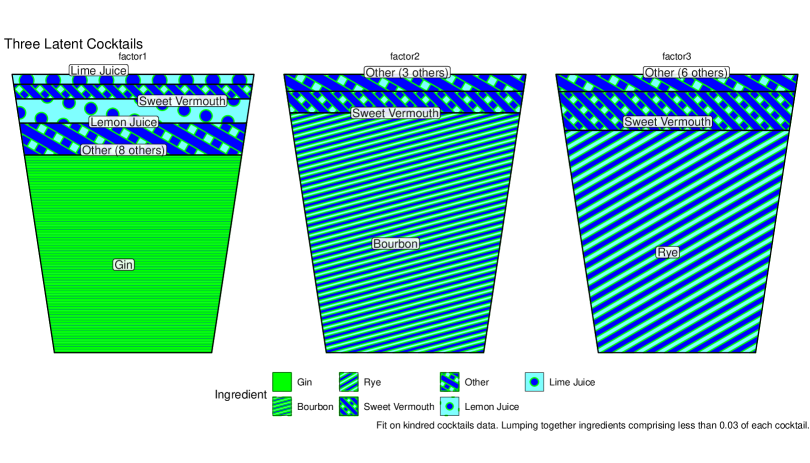
While the table is definitive, it is hard to appreciate the distribution of ingredients in the latent factor cocktails. Towards that end, we plot them in stacked barcharts in Figure 4. These barcharts are styled to look like drinks, what one might call “tumbler plots”. We notice that the latent factor cocktails contain a large number of ingredients falling under the display limit of 0.03. We also see repetition of ingredients in the factor cocktails, with Sweet Vermouth appearing in appreciable amounts in all three.

To remedy that, we fit again, this time using λ1,L=λ1,R=0.4\lambda_{1,L}=\lambda_{1,R}=0.4 and γ2,R=0.25\gamma_{2,R}=0.25. It is important to note that because we decompose 𝖸𝖫𝖱\mathsf{Y}\approx\mathsf{L}\mathsf{R} that applying an 1\ell_{1} penalty solely on 𝖱\mathsf{R} could result in a rescaling of output such that elements of 𝖱\mathsf{R} are small in magnitude and elements of 𝖫\mathsf{L} are large. That is, because 𝖫𝖱=(𝖫𝖰)(𝖰1𝖱)\mathsf{L}\mathsf{R}=\left(\mathsf{L}\mathsf{Q}\right)\left({{\mathsf{Q}}^{-1}}\mathsf{R}\right), we could take 𝖰=v𝖨\mathsf{Q}=v\mathsf{I} for large vv and make the 1\ell_{1} penalty on 𝖱\mathsf{R} irrelevant without really making the decomposition sparse. To address this, one mst typically apply an 1\ell_{1} penalty to both 𝖫\mathsf{L} and 𝖱\mathsf{R} as we do here.

We chose the values of λ1,L,λ1,R,γ2,R\lambda_{1,L},\lambda_{1,R},\gamma_{2,R} by trial and error, as unfortunately there is no theory to guide us here. Forging on, we plot the results in Figure 5. We see there that the factor cocktails are now contain far fewer ingredients, though they all hew to the formula of base spirit plus vermouth, with some extras. These seem more “spirit-forward” than a typical cocktail, but de gustibus non est disputandum.

Refer to caption
Figure 5: The second fit of three latent cocktails are shown. Ingredients making less than 0.03 of the total lumped together.

Finally, we perform another fit, this time with d=9d=9, and using λ1,L=λ1,R=0.5\lambda_{1,L}=\lambda_{1,R}=0.5, λ2,L=λ2,R=2.5\lambda_{2,L}=\lambda_{2,R}=2.5, γ2,R=0.25\gamma_{2,R}=0.25, values again chosen by trial and error. We plot the results of this fit in Figure 6. Again we see heavy use of base spirits with a sprinkling of secondary ingredients. One can imagine in the limit as dd approaches the number of base ingredients that the factorization could collapse to the trivial one 𝖸=𝖸𝖨\mathsf{Y}=\mathsf{Y}\mathsf{I}. We see that behavior here with the top nine most popular ingredients dominating the latent factor cocktails. Thus it is hard to view non-negative matrix factorization as a good way of quantifying and describing the space of cocktails. Probably a better approach would be to recognize that cocktails evolve from other cocktails, then try to infer and describe the evolutionary structure.

Refer to caption
Figure 6: The nine latent cocktails are shown. Ingredients making less than 0.03 of the total lumped together.

References

Appendix A Matrix Identities

The following identities are useful for switching between matrix and vectorized representations. [11]

vec(𝖡𝖢𝖣)\displaystyle\operatorname{vec}\left(\mathsf{B}\mathsf{C}\mathsf{D}\right) =(𝖣𝖡)vec(𝖢).\displaystyle=\left({{{\mathsf{D}}^{\top}}}\otimes{\mathsf{B}}\right)\operatorname{vec}\left(\mathsf{C}\right). (27)
tr(𝖠𝖢)\displaystyle\operatorname{tr}\left({{\mathsf{A}}^{\top}}\mathsf{C}\right) =vec(𝖠)vec(𝖢).\displaystyle={{\operatorname{vec}\left(\mathsf{A}\right)}^{\top}}\operatorname{vec}\left(\mathsf{C}\right). (28)
tr(𝖠𝖡𝖢𝖣)\displaystyle\operatorname{tr}\left({{\mathsf{A}}^{\top}}\mathsf{B}\mathsf{C}\mathsf{D}\right) =vec(𝖠)(𝖣𝖡)vec(𝖢).\displaystyle={{\operatorname{vec}\left(\mathsf{A}\right)}^{\top}}\left({{{\mathsf{D}}^{\top}}}\otimes{\mathsf{B}}\right)\operatorname{vec}\left(\mathsf{C}\right). (29)
tr(𝖠𝖡𝖠𝖣)\displaystyle\operatorname{tr}\left({{\mathsf{A}}^{\top}}\mathsf{B}\mathsf{A}\mathsf{D}\right) =vec(𝖠)𝖣𝖡2.\displaystyle=\left\|{\operatorname{vec}\left(\mathsf{A}\right)}\right\|_{{{{\mathsf{D}}^{\top}}}\otimes{\mathsf{B}}}^{2}. (30)
(𝖠𝖡)\displaystyle{{\left({\mathsf{A}}\otimes{\mathsf{B}}\right)}^{\top}} =𝖠𝖡.\displaystyle={{{\mathsf{A}}^{\top}}}\otimes{{{\mathsf{B}}^{\top}}}. (31)