An Online Newton’s Method for Time-varying Linear Equality Constraints

Jean-Luc Lupien and Antoine Lesage-Landry IEEE Member J.-L. Lupien and A. Lesage-Landry are with the Department of Electrical Engineering, Polytechnique Montréal, GERAD & Mila, Montréal, QC, Canada, H3T 1J4. e-mail: {jean-luc.lupien, antoine.lesage-landry}@polymtl.ca.This work was funded by the Institute for Data Valorization (IVADO) and the Natural Sciences and Engineering Research Council (NSERC).

Abstract

We consider online optimization problems with time-varying linear equality constraints. In this framework, an agent makes sequential decisions using only prior information. At every round, the agent suffers an environment-determined loss and must satisfy time-varying constraints. Both the loss functions and the constraints can be chosen adversarially. We propose the Online Projected Equality-constrained Newton Method (OPEN-M) to tackle this family of problems. We obtain sublinear dynamic regret and constraint violation bounds for OPEN-M under mild conditions. Namely, smoothness of the loss function and boundedness of the inverse Hessian at the optimum are required, but not convexity. Finally, we show OPEN-M outperforms state-of-the-art online constrained optimization algorithms in a numerical network flow application.

{IEEEkeywords}

Optimization algorithms, Time-varying systems, Machine learning

1 Introduction

\IEEEPARstart

In online convex optimization (OCO), an agent aims to sequentially play the best decision with respect to a potentially adversarial loss function using only prior information [1, 2]. In other words, decisions must be made before observing the loss function and constraints. OCO algorithms have many applications including portfolio selection, artificial intelligence, and real-time control of power systems [3, 4, 5].

The preponderant performance metric for OCO algorithms is regret [1], the cumulative difference between the loss incurred by the agent and that of a comparator sequence. Two main types of regret exist: static and dynamic. For static regret, the comparator sequence is defined as the best fixed decision in hindsight [2]. For dynamic regret, the comparator sequence is the round-optimal decision in hindsight [2, 4]. In OCO, one intends to design an algorithm that possesses a sublinear regret bound. Sublinear regret implies that the time-averaged regret goes to zero as time increases. The OCO algorithm therefore plays the best decision with respect to the comparator sequence over sufficiently long time horizons [1, 4].

A persistent obstacle in OCO algorithmic design has been the integration of time-varying constraints. In this context, the decision sequence must also satisfy environment-determined constraints [6]. The performance of such algorithms is measured both in terms of its regret but also its constraint violation, the cumulative distance from feasibility of the agent’s decisions. Similarly to the regret, a sublinear constraint violation is desired and implies that, on average, decisions will be feasible over a large time horizon [7]. When considering time-varying constraints, an analysis using the dynamic regret is preferable over one based on the static regret because the best fixed feasible decision can have an arbitrarily large loss or might not even exist [8].

Most OCO algorithms tackling time-varying constraints are analysed based only on static regret. In [7, 8] and [9], sublinear regret and violation bounds are achieved for long-term constraints. Sublinear static regret and constraint violation bounds are also achieved in [10] using virtual queues and in [11] using an online saddle-point algorithm. More recently, an augmented Lagrangian method [12] has been shown to outperform previous Lagragian-based methods [6, 11, 10] in numerical experiments.

Algorithms with dynamic regret bounds have also been developed such as the modified online saddle-point method (MOSP) [6]. This algorithm has simultaneous sublinear dynamic regret and constraint violation bounds. However, MOSP’s bounds are dependent on strict conditions on optimal primal and dual variable variations in addition to time-sensitive step sizes. An exact-penalty method for dealing with time-varying constraints possessing sublinear regret and constraint violation bounds was presented in [13] but shares MOSP’s step size limitation. Virtual queues are used in [14] with time-varying constraints achieving simultaneous sublinear regret and constraint violation bounds without requiring Slater’s condition to hold. Sublinear regret and constraint violation are achieved in [15] including for some non-convex functions but with considerably looser bounds.

The application of an interior-point method to time-varying convex optimization is presented in [16]. However, this context differs from OCO because current-round information is available to the decision-maker.

In this work, our main contribution is the design of a novel online optimization algorithm that can efficiently deal with time-varying linear equality constraints in the OCO setting. This method simultaneously possesses the tightest dynamic regret and constraint violation bounds presented thus far for constrained OCO problems. Additionally, the method does not require hyperparameters, time-dependent step sizes, or a predefined time horizon making it easily implementable.

2 Background

In recent work, a second-order method for online optimization yielded tighter dynamic regret bounds compared to first-order approaches [17]. Specifically, [17] proposes an online extension of Newtons’ method, ONM, applicable to non-convex problems that possesses a tight dynamic regret bound. However, this approach is only applicable to unconstrained problems. In an offline setting, the unconstrained and linear equality-constrained Newton’s method’s performance are the same [18, 19]. This result motivates the extension of ONM to a setting with time-varying linear equality constraints.

2.1 Problem definition

We consider online optimization problems of the following form. Let $\mathbf{x}_{t}\in\mathbb{R}^{n}$ , $n\in\mathbb{N}$ be the decision vector at time $t$ . Let $f_{t}$ : $\mathbb{R}^{n}\mapsto\mathbb{R}$ be a twice-differentiable function. Let $\mathbf{A}_{t}\in\mathbb{R}^{p\times n}$ be a rank $p\in\mathbb{N}$ full row-rank matrix, and $\mathbf{b}_{t}\in\mathbb{R}^{p}$ . The problem at round $t=1,2,...,T$ can then be written as:

\displaystyle\begin{split}&\min\limits_{\mathbf{x}_{t}}f_{t}(\mathbf{x}_{t})\\ \text{s.t.}\quad&\mathbf{A}_{t}\mathbf{x}_{t}=\mathbf{b}_{t}.\end{split}

(1)

In this work, dynamic regret will be used as the performance metric because it is more stringent compared to static regret. Indeed, sublinear dynamic regret implies sublinear static regret [8]. Dynamic regret $R_{\text{d}}(T)$ is defined as:

\displaystyle R_{\text{d}}(T)=\sum\limits_{t=1}^{T}\big{[}f_{t}(\mathbf{x}_{t})-f_{t}(\mathbf{x}^{*}_{t})\big{]},

(2)

where $\mathbf{x}_{t}^{*}$ is the round-optimal solution and $T\in\mathbb{N}$ is the time horizon. For (1), the round-optimum $\mathbf{x}_{t}^{*}$ is the solution to the following system of equations:

	$\displaystyle\nabla f_{t}(\mathbf{x}^{}_{t})+\mathbf{A}_{t}^{\top}\bm{\nu}^{}_{t}$	$\displaystyle=0$
	$\displaystyle\mathbf{A}_{t}\mathbf{x}^{*}_{t}-\mathbf{b}_{t}$	$\displaystyle=0,$

where $\bm{\nu}_{t}^{*}\in\mathbb{R}^{n}$ is the dual variable associated with (1)’s equality constraints.

The constraint violation term is defined as:

\displaystyle\text{Vio}(T)=\sum\limits_{t=1}^{T}\left\lVert\mathbf{A}_{t}\mathbf{x}_{t}-\mathbf{b}_{t}\right\rVert,

(3)

and quantifies the cumulative distance from feasibility, with respect to the Euclidean norm, of the decision sequence. All norms, $\left\lVert\cdot\right\rVert$ , refer to the Euclidean norm in the sequel. Constraint violation is zero if decisions are feasible at all rounds. This definition is similar to that used in [6, 15] and is stricter than in [12] and [14] because the constraints must be satisfied at every timestep and not on average.

In the first part of this work, we investigate the case for which the feasible space is the same for all rounds, i.e., $\mathbf{A}_{t}=\mathbf{A},\mathbf{b}_{t}=\mathbf{b}$ for all $t$ . The second part builds on this result and extends it to time-varying equality constraints.

2.2 Preliminaries

We define the function $\mathbf{D}_{t}(\mathbf{x}):\mathbb{R}^{n}\mapsto\mathbb{R}^{(n+p)^{2}}$ as:

\mathbf{D}_{t}(\mathbf{x})=\begin{bmatrix}\nabla^{2}f_{t}(\mathbf{x})&\mathbf{A}^{\top}_{t}\\ \mathbf{A}_{t}&0\end{bmatrix},

where $\nabla^{2}f_{t}(\mathbf{x})$ is the Hessian matrix of $f_{t}$ . We assume that the Hessian is invertible for all $t$ which implies that $\mathbf{D}_{t}(\mathbf{x})$ is also invertible [18, Section 10.1]. This guarantees that the Newton update is defined at every round.

Next, we present the online equality-constrained Newton (OEN) update. For any feasible point $\mathbf{x}_{t}$ , the OEN update minimizes the second-order approximation of $f_{t}$ around $\mathbf{x}_{t}$ subject to the equality constraints. An estimate of the optimal dual variable, $\bm{\nu}_{t}$ , is also obtained from the update.

Definition 1 (OEN update)

The OEN update is:

\displaystyle\begin{split}\begin{bmatrix}\Delta\mathbf{x}_{t}\\ \bm{\nu}_{t}\end{bmatrix}&=-\mathbf{D}_{t}^{-1}(\mathbf{x}_{t})\begin{bmatrix}\nabla f_{t}(\mathbf{x}_{t})\\ 0\end{bmatrix}\\ \mathbf{x}_{t+1}&=\mathbf{x}_{t}+\Delta\mathbf{x}_{t}.\end{split}

(4)

Let $\mathbf{v}_{t}\in\mathbb{R}^{n}$ be the difference between subsequent optima: $\mathbf{v}_{t}=\mathbf{x}_{t+1}^{*}-\mathbf{x}_{t}^{*}$ . Throughout this work, we assume: $0\leq\left\lVert\mathbf{v}_{t}\right\rVert\leq\overline{v}$ for all $t$ . This limits the variation in optima between two subsequent rounds. It is a common assumption in dynamic OCO [6, 17, 15]. This assumption could be satisfied in real-world applications such as electric grids where the temporal continuity imposed by the underlying physics limits the variation in optima provided the timestep is sufficiently small. The total variation $V_{T}$ is defined as:

V_{T}=\sum\limits_{t=0}^{T-1}\left\lVert\mathbf{x}_{t+1}^{*}-\mathbf{x}_{t}^{*}\right\rVert=\sum\limits_{t=0}^{T-1}\left\lVert\mathbf{v}_{t}\right\rVert,

and is bounded above by $V_{T}\leq\overline{v}T$ .

An important tool for the analysis of the OEN update is the reduced function $\tilde{f}_{t}(\mathbf{z}):\mathbb{R}^{n-p}\mapsto\mathbb{R}$ which is a representation of $f_{t}(\mathbf{x})$ over the feasible set.

Let $\mathbf{F}_{t}\in\mathbb{R}^{n\times(n-p)}$ be such that $\mathcal{R}(\mathbf{F}_{t})=\mathcal{N}(\mathbf{A}_{t})$ where $\mathcal{R}$ is the column space of a matrix and $\mathcal{N}$ is its null space. Let $\mathbf{\hat{x}}\in\mathbb{R}^{n}$ be such that $\mathbf{A}_{t}\mathbf{\hat{x}}-\mathbf{b}_{t}=\mathbf{0}$ . Then, $\tilde{f}_{t}$ is defined as:

\tilde{f_{t}}(\mathbf{z})=f_{t}(\mathbf{F}_{t}\mathbf{z}+\mathbf{\hat{x}}).

We remark that the reduced function shares minima with $f_{t}$ , i.e., $\min\limits_{\mathbf{z}}\tilde{f_{t}}(\mathbf{z})=f_{t}(\mathbf{x}_{t}^{*})$ [18]. This gives rise to an equivalent unconstrained, reduced problem: $\min\limits_{\mathbf{z}}\tilde{f}_{t}(\mathbf{z})$ , which can be solved using ONM [17].

Additionally, there exists a unitary matrix $\overline{\mathbf{F}}_{t}\in\mathbb{R}^{n\times(n-p)}$ such that $\mathcal{R}\left(\overline{\mathbf{F}}_{t}\right)=\mathcal{N}(\mathbf{A}_{t})$ . Without loss of generality, we let $\mathbf{F}_{t}=\overline{\mathbf{F}}_{t}$ in our analysis. It follows that for any $\mathbf{z}_{t}$ satisfying $\mathbf{x}_{t}=\overline{\mathbf{F}}_{t}\mathbf{z}_{t}+\mathbf{\hat{x}}$ , we have $\left\lVert\mathbf{x}_{t}-\mathbf{x}_{t}^{*}\right\rVert=\left\lVert\overline{\mathbf{F}}_{t}(\mathbf{z}_{t}-\mathbf{z}_{t}^{*})\right\rVert=\left\lVert\mathbf{z}_{t}-\mathbf{z}_{t}^{*}\right\rVert$ . In other words, the norm of the original problem’s OEN update and the reduced problem’s ONM update coincide when $\mathbf{F}_{t}=\overline{\mathbf{F}}_{t}$ .

2.3 Assumptions

We now introduce three recurring assumptions that are used throughout this work. These assumptions are mild and notably do not require the objective function to be convex. These assumptions must hold for all $t=1,2,3,...,T$ .

Assumption 1

There exists a constant $h>0$ such that:

\left\lVert\nabla^{2}f_{t}(\mathbf{x}_{t}^{*})^{-1}\right\rVert\leq\frac{1}{h}.

Assumption 2

There exists non-negative finite constants $\beta>0$ and $0<L<+\infty$ such that:

\left\lVert\mathbf{x}-\mathbf{x}_{t}^{*}\right\rVert\leq\beta\Rightarrow\\ \left\lVert\nabla^{2}f_{t}(\mathbf{x})-\nabla^{2}f_{t}(\mathbf{x}_{t}^{*})\right\rVert\leq L\left\lVert\mathbf{x}-\mathbf{x}_{t}^{*}\right\rVert.

Assumption 3

There exists $0<l<+\infty$ such that:

\left\lVert f_{t}(\mathbf{x})-f_{t}(\mathbf{x}^{*}_{t})\right\rVert\leq l\left\lVert\mathbf{x}-\mathbf{x}^{*}_{t}\right\rVert.

Assumption 1 imposes an upper bound on the norm of the inverse Hessian at the optimum. This implies that the Hessian’s eigenvalues can be positive or negative but must be bounded away from zero. For convex loss functions, this is equivalent to strong convexity which is a common assumption in OCO [1, 17, 10]. Assumptions 2 and 3 are local Lipschitz continuity conditions on the objective function and its Hessian around the optimum.

2.4 Reduced function identities

We now provide two lemmas which characterize the reduced function $\tilde{f}_{t}$ .

Lemma 1

[18, Section 10.2.3] Suppose

1.

$\exists\mathbf{F}_{t}\text{ such that }\mathcal{N}(\mathbf{A}_{t})=\mathcal{R}(\mathbf{F}_{t});$
2.

$\exists\mathbf{\hat{x}}\text{ such that }\mathbf{A}_{t}\mathbf{\hat{x}}=\mathbf{b}_{t};$
3.

$\mathbf{A}_{t}\mathbf{x}_{t}-\mathbf{b}_{t}=\mathbf{0}.$

Consider the Newton step applied to the reduced function $\tilde{f}_{t}(\mathbf{z}_{t})$ : $\Delta\mathbf{z}_{t}=-\nabla^{2}\tilde{f_{t}}(\mathbf{z}_{t})^{-1}\nabla\tilde{f_{t}}(\mathbf{z}_{t})$ . Then the following identity holds :

\displaystyle\Delta\mathbf{x}_{t}=\mathbf{F}_{t}\Delta\mathbf{z}_{t}.

(5)

Lemma 1 implies that the Newton step applied to the constrained problem coincides with the Newton step applied to the reduced problem. By setting $\mathbf{F}_{t}=\overline{\mathbf{F}}_{t}$ , we obtain $\left\lVert\Delta\mathbf{x}_{t}\right\rVert=\left\lVert\Delta\mathbf{z}_{t}\right\rVert$ .

The second lemma characterizes the local strong convexity and Lipschitz continuity of the reduced function.

Lemma 2

Suppose Assumptions 1 and 2 hold. Then we have:

		$\displaystyle\left\lVert\nabla^{2}\tilde{f}_{t}(\mathbf{z}_{t}^{*})^{-1}\right\rVert\leq\frac{1}{\sigma_{\min}(\mathbf{F}_{t})^{2}h}$		(6)
		$\displaystyle\left\lVert\mathbf{z}-\mathbf{z}^{*}_{t}\right\rVert\leq\frac{\beta}{\left\lVert\mathbf{F}_{t}\right\rVert}\Rightarrow$
		$\displaystyle\quad\left\lVert\nabla^{2}\tilde{f_{t}}(\mathbf{z})-\nabla^{2}\tilde{f_{t}}(\mathbf{z}_{t}^{})\right\rVert\leq L\left\lVert\mathbf{F}_{t}\right\rVert^{3}\left\lVert\mathbf{z}-\mathbf{z}_{t}^{}\right\rVert,$		(7)

where $\sigma_{\min}(\mathbf{F}_{t})$ is the minimum singular value of $\mathbf{F}_{t}$ .

Proof 2.2.

Differentiating $\tilde{f}_{t}$ twice, we obtain,

\nabla^{2}\tilde{f_{t}}(\mathbf{z})=\mathbf{F}_{t}\nabla^{2}f_{t}(\mathbf{x}_{t}^{*})\mathbf{F}_{t}^{\top}.

The inverse Hessian of $\tilde{f}_{t}$ is thus upper bounded by:

	$\displaystyle\left\lVert\nabla^{2}\tilde{f}_{t}(\mathbf{z}^{*})^{-1}\right\rVert$	$\displaystyle=\left\lVert\mathbf{F}_{t}(\mathbf{F}_{t}^{\top}\mathbf{F}_{t})^{-1}\nabla^{2}f_{t}(\mathbf{x}_{t}^{*})^{-1}(\mathbf{F}_{t}^{\top}\mathbf{F}_{t})^{-1}\mathbf{F}_{t}^{\top}\right\rVert$
		$\displaystyle\leq\left\lVert(\mathbf{F}_{t}^{\top}\mathbf{F}_{t})^{-1}\mathbf{F}_{t}^{\top}\right\rVert^{2}\left\lVert\nabla^{2}f_{t}(\mathbf{x}_{t}^{*})^{-1}\right\rVert$
		$\displaystyle\leq\frac{1}{\sigma_{\min}(\mathbf{F}_{t})^{2}h},$

which is (6).
For (7), we have,

	$\displaystyle\left\lVert\nabla^{2}\tilde{f_{t}}(\mathbf{z})-\nabla^{2}\tilde{f_{t}}(\mathbf{z}_{t}^{*})\right\rVert$	$\displaystyle=\big{\\|}\mathbf{F}_{t}\big{(}\nabla^{2}f_{t}(\mathbf{F}_{t}\mathbf{z}+\mathbf{\hat{x}})-$
		$\displaystyle\quad\quad\quad\nabla^{2}f_{t}(\mathbf{F}_{t}\mathbf{z}^{*}_{t}+\mathbf{\hat{x}})\big{)}\mathbf{F}_{t}^{\top}\big{\\|}$
		$\displaystyle\leq\left\lVert\mathbf{F}_{t}\right\rVert^{2}\big{\\|}\nabla^{2}f_{t}(\mathbf{F}_{t}\mathbf{z}+\mathbf{\hat{x}})-$
		$\displaystyle\quad\quad\quad\quad\nabla^{2}f_{t}(\mathbf{F}_{t}\mathbf{z}^{*}_{t}+\mathbf{\hat{x}})\big{\\|}$
		$\displaystyle\leq\left\lVert\mathbf{F}_{t}\right\rVert^{2}L\left\lVert\mathbf{F}_{t}(\mathbf{z}-\mathbf{z}^{*}_{t})\right\rVert$
		$\displaystyle\leq L\left\lVert\mathbf{F}_{t}\right\rVert^{3}\left\lVert\mathbf{z}-\mathbf{z}^{*}_{t}\right\rVert,$

where the last inequalities follow from the Lipschitz continuity of $\nabla^{2}f_{t}$ and the definition of $\mathbf{z}_{t}$ , respectively.

2.5 Feasible Newton update

Using Lemmas 1 and 2, we derive the following lemma for the original constrained problem:

Lemma 2.3 (Equality-constrained Newton identities).

Suppose Assumptions 1, 2 hold and:

1.

$\left\lVert\mathbf{x}_{t}-\mathbf{x}_{t}^{*}\right\rVert\leq\min\left\{\beta,\frac{h}{2L}\right\};$
2.

$\mathbf{A}_{t}\mathbf{x}_{t}-\mathbf{b}_{t}=\mathbf{0}.$

Then we have the following two identities for OEN:

	$\displaystyle\left\lVert\mathbf{x}_{t+1}-\mathbf{x}_{t}^{*}\right\rVert$	$\displaystyle<\left\lVert\mathbf{x}_{t}-\mathbf{x}_{t}^{*}\right\rVert;$		(8)
	$\displaystyle\left\lVert\mathbf{x}_{t+1}-\mathbf{x}_{t}^{*}\right\rVert$	$\displaystyle\leq\frac{2L}{h}\left\lVert\mathbf{x}_{t}-\mathbf{x}_{t}^{*}\right\rVert.$		(9)

The first inequality guarantees the next iterate is strictly closer to the optimum compared to the current iterate. The second inequality provides an upper bound on this value.

Proof 2.4.

By the definition of the OEN update and Lemma 1 we have:

\mathbf{x}_{t+1}-\mathbf{x}_{t}^{*}=\mathbf{x}_{t}-\mathbf{x}_{t}^{*}-\mathbf{F}_{t}\nabla^{2}\tilde{f}_{t}(\mathbf{z}_{t})^{-1}\nabla\tilde{f}_{t}(\mathbf{z}_{t}).

Rearranging and letting $\mathbf{F}_{t}=\overline{\mathbf{F}}_{t}$ , we have

	$\displaystyle\mathbf{x}_{t+1}-\mathbf{x}_{t}^{*}$	$\displaystyle=\mathbf{x}_{t}-\mathbf{x}_{t}^{*}-$
		$\displaystyle\quad\quad\quad\overline{\mathbf{F}}_{t}\nabla^{2}\tilde{f}_{t}(\mathbf{z}_{t})^{-1}\big{(}\nabla\tilde{f}_{t}(\mathbf{z}_{t})-\nabla\tilde{f}_{t}(\mathbf{z}_{t}^{*})\big{)}$
		$\displaystyle=\mathbf{x}_{t}-\mathbf{x}_{t}^{*}-\overline{\mathbf{F}}_{t}\nabla^{2}\tilde{f}_{t}(\mathbf{z}_{t})^{-1}\cdot$
		$\displaystyle\quad\quad\quad\int_{0}^{1}\nabla^{2}\tilde{f}_{t}\big{(}\mathbf{z}_{t}+\tau(\mathbf{z}_{t}^{}-\mathbf{z}_{t})\big{)}(\mathbf{z}_{t}^{}-\mathbf{z}_{t})\text{d}\tau.$

From the symmetry of the Hessian and its inverse we have,

	$\displaystyle\mathbf{x}_{t+1}-\mathbf{x}_{t}^{*}$	$\displaystyle=\mathbf{x}_{t}-\mathbf{x}_{t}^{}-\overline{\mathbf{F}}_{t}(\mathbf{z}_{t}^{}-\mathbf{z}_{t})\nabla^{2}\tilde{f}_{t}(\mathbf{z}_{t})^{-1}\cdot$
		$\displaystyle\quad\quad\quad\quad\quad\int_{0}^{1}\nabla^{2}\tilde{f}_{t}\big{(}\mathbf{z}_{t}+\tau(\mathbf{z}_{t}^{*}-\mathbf{z}_{t})\big{)}\text{d}\tau$
		$\displaystyle=(\mathbf{x}_{t}^{*}-\mathbf{x}_{t})\nabla^{2}\tilde{f}_{t}(\mathbf{z})^{-1}\cdot$
		$\displaystyle\quad\quad\int_{0}^{1}\Big{[}\nabla^{2}\tilde{f}_{t}\big{(}\mathbf{z}+\tau(\mathbf{z}^{*}-\mathbf{z})\big{)}-\nabla^{2}\tilde{f}_{t}(\mathbf{z})\Big{]}\text{d}\tau.$

Taking the norm on both sides and using Lemmas 1 and 2 yields

	$\displaystyle\left\lVert\mathbf{x}_{t+1}-\mathbf{x}_{t}^{*}\right\rVert$	$\displaystyle\leq\left\lVert\mathbf{x}_{t}^{*}-\mathbf{x}_{t}\right\rVert\left\lVert\nabla^{2}\tilde{f}_{t}(\mathbf{z})^{-1}\right\rVert\mathbf{\cdot}$
		$\displaystyle\quad\int_{0}^{1}\left\lVert\nabla^{2}\tilde{f}_{t}\big{(}\mathbf{z}+\tau(\mathbf{z}^{*}-\mathbf{z})\big{)}+\nabla^{2}\tilde{f}_{t}(\mathbf{z})\right\rVert\text{d}\tau$

	$\displaystyle\leq\left\lVert\mathbf{x}_{t}^{*}-\mathbf{x}_{t}\right\rVert\left\lVert\nabla^{2}\tilde{f}_{t}(\mathbf{z})^{-1}\right\rVert$
	$\displaystyle\quad\quad\quad\int_{0}^{1}2L\left\lVert\overline{\mathbf{F}}_{t}\right\rVert^{2}\tau\left\lVert\mathbf{x}_{t}^{*}-\mathbf{x}_{t}\right\rVert\text{d}\tau$
	$\displaystyle\leq\left\lVert\nabla^{2}\tilde{f}_{t}(\mathbf{z})^{-1}\right\rVert L\left\lVert\mathbf{x}_{t}^{*}-\mathbf{x}_{t}\right\rVert^{2}.$		(10)

Using [17, Lemma 2], we can bound the inverse Hessian as:

	$\displaystyle\left\lVert\nabla^{2}\tilde{f}(\mathbf{z})^{-1}\right\rVert$	$\displaystyle\leq\frac{1}{\sigma_{\min}(\overline{\mathbf{F}}_{t})^{2}h-L\left\lVert\overline{\mathbf{F}}_{t}\right\rVert^{2}\left\lVert\mathbf{x}^{*}_{t}-\mathbf{x}_{t}\right\rVert}$
		$\displaystyle\leq\frac{1}{h-L\left\lVert\mathbf{x}^{*}_{t}-\mathbf{x}_{t}\right\rVert},$		(11)

because $\sigma_{\min}(\overline{\mathbf{F}}_{t})=\left\lVert\overline{\mathbf{F}}_{t}\right\rVert=1$ . Substituting (10) into (11) leads to:

\displaystyle\left\lVert\mathbf{x}_{t+1}-\mathbf{x}_{t}^{*}\right\rVert

\displaystyle\leq\frac{L}{h-L\left\lVert\mathbf{x}_{t}^{*}-\mathbf{x}_{t}\right\rVert}\left\lVert\mathbf{x}_{t}^{*}-\mathbf{x}_{t}\right\rVert^{2}

(12)

Finally, (8) and (9) follows from (12) and [17, Lemma 2]’s proof.

3 Online Equality-constrained Newton’s Method

We now present our online optimization methods for problems with time-independent and time-varying equality constraints.

3.1 Online Equality-constrained Newton’s Method

In this section, we propose the Online Equality-constrained Newton’s Method (OEN-M) for online optimization subject to time-invariant linear equality constraints. This is the first online, second-order algorithm that admits constraints. OEN-M is presented in Algorithm 1.

Algorithm 1 Online Equality-constrained Newton’s Method

Parameters:

\mathbf{A}

\mathbf{b}

Initialization: Receive

\mathbf{x}_{0}\in\mathbb{R}

such that

\left\lVert\mathbf{x}_{0}-\mathbf{x}_{0}^{*}\right\rVert\leq\gamma=\min\left\{\beta,\frac{h}{2L}\right\}

and

\mathbf{A}\mathbf{x}_{0}-\mathbf{b}=\mathbf{0}

for

t=0,1,2...T

Play the decision

\mathbf{x}_{t}

Observe the outcome

f_{t}(\mathbf{x}_{t})

Update decision:

\begin{bmatrix}\mathbf{x}_{t+1}\\ \bm{\nu}_{t}\end{bmatrix}

=\begin{bmatrix}{\mathbf{x}}_{t}\\ \mathbf{0}\end{bmatrix}-\mathbf{D}_{t}({\mathbf{x}}_{t})^{-1}\begin{bmatrix}\nabla f_{t}(\mathbf{x}_{t})\\ \mathbf{0}\end{bmatrix}

end for

We now show that OEN-M has a dynamic regret bounded above by $O(V_{T}+1)$ and a null constraint violation.

Theorem 3.5.

If Assumptions 1 $-$ 3 hold and the following conditions are respected:

1.

$\exists\mathbf{x}_{0}\text{ such that }\left\lVert\mathbf{x}_{0}-\mathbf{x}_{0}^{*}\right\rVert\leq\gamma=\min\{\beta,\frac{h}{2L}\}$ ;
2.

$\overline{v}\leq\gamma-\frac{2L}{h}\gamma^{2}$ .

Then the regret $R_{\text{d}}(T)$ and the constraint violation $\text{Vio}(T)$ are bounded above by :

	$\displaystyle R_{\text{d}}(T)$	$\displaystyle\leq\frac{lh}{h-2L\gamma}(V_{T}+\delta);$		(13)
	$\displaystyle\text{Vio}(T)$	$\displaystyle=0.$		(14)

Remark 3.6.

The assumption that the decision-maker has access to $\mathbf{x}_{0}$ such that $\left\lVert\mathbf{x}_{0}-\mathbf{x}_{0}^{*}\right\rVert\leq\gamma$ is standard in OCO [11, 17, 15]. Essentially, this means obtaining a good starting estimate of the initial optimal solution is required. It is assumed that a good estimate can be obtained before the start of the online process from, for example, offline calculations or a previously implemented decision.

Proof 3.7.

Using Assumption 3, the regret is bounded by:

R_{\text{d}}(T)=\sum\limits_{t=1}^{T}\big{|}f_{t}(\mathbf{x}_{t})-f_{t}(\mathbf{x}_{t}^{*})\big{|}\leq l\sum\limits_{t=1}^{T}\left\lVert\mathbf{x}_{t}-\mathbf{x}_{t}^{*}\right\rVert.

(15)

Rearranging (15)’s sum we obtain:

	$\displaystyle\sum\limits_{t=1}^{T}\left\lVert\mathbf{x}_{t}-\mathbf{x}_{t}^{*}\right\rVert$	$\displaystyle=\sum\limits_{t=1}^{T}\left\lVert\mathbf{x}_{t}-\mathbf{x}_{t-1}^{}+\mathbf{x}^{}_{t-1}-\mathbf{x}_{t}^{*}\right\rVert$
		$\displaystyle\leq\sum\limits_{t=1}^{T}\left\lVert\mathbf{x}_{t}-\mathbf{x}_{t-1}^{}\right\rVert+\sum\limits_{t=1}^{T}\left\lVert\mathbf{x}_{t}^{}-\mathbf{x}_{t-1}^{*}\right\rVert$
		$\displaystyle\leq\sum\limits_{t=0}^{T-1}\frac{2L}{h}\left\lVert\mathbf{x}_{t}-\mathbf{x}_{t}^{*}\right\rVert^{2}+V_{T}$
		$\displaystyle\leq\sum\limits_{t=1}^{T}\frac{2L}{h}\gamma\left\lVert\mathbf{x}_{t}-\mathbf{x}_{t}^{*}\right\rVert+V_{T}+\delta,$

where $\delta=\frac{2L}{h}\gamma(\left\lVert\mathbf{x}_{0}-\mathbf{x}_{0}^{*}\right\rVert-\left\lVert\mathbf{x}_{T}-\mathbf{x}_{T}^{*}\right\rVert)$ . Solving for $\left\lVert\mathbf{x}_{t}-\mathbf{x}_{t}^{*}\right\rVert$ , we have:

\displaystyle\sum\limits_{t=1}^{T}\left\lVert\mathbf{x}_{t}-\mathbf{x}_{t}^{*}\right\rVert

\displaystyle\leq\left(1-\frac{2L}{h}\gamma\right)^{-1}(V_{T}+\delta).

(16)

This implies that the dynamic regret is bounded above by:

\displaystyle R_{\text{d}}(T)\leq\frac{lh}{h-2L\gamma}(V_{T}+\delta),

and hence, $R_{\text{d}}(T)\leq O(V_{T}+1)$ .

As for the constraint violation, we have that $\mathbf{x}_{0}$ is feasible by assumption. Because every OEN update is such that $\mathbf{A}\Delta\mathbf{x}=0$ , every subsequent decision will also be feasible. We thus have:

\displaystyle\text{Vio}(T)

\displaystyle=\sum\limits_{t=1}^{T}\left\lVert\mathbf{A}\mathbf{x}_{t}-\mathbf{b}\right\rVert=0,

which completes the proof.

3.2 Online Projected Newton’s Method

We now consider online optimization problems with time-varying equality constraints. OEN does not apply to this class of problems because the previously played decision might not be feasible under the new constraints. We propose the Online Projected Equality-constrained Newton’s Method (OPEN-M) to address this limitation. OPEN-M consists of a projection of the previous decision onto the new feasible set followed by an OEN step from this point. OPEN-M is detailed in Algorithm 2.

Algorithm 2 Online Projected Eq.-const. Newton Method

Initialization: Receive

\mathbf{x}_{0}\in\mathbb{R}

such that

\left\lVert\mathbf{x}_{0}-\mathbf{x}_{0}^{*}\right\rVert\leq\gamma=\min\left\{\beta,\frac{h}{2L}\right\}

for

t=0,1,2...T

Play the decision

\mathbf{x}_{t}.

Observe the outcome

f_{t}(\mathbf{x}_{t})

and constraints

\mathbf{A}_{t},\mathbf{b}_{t}

Project

\mathbf{x}_{t}

onto the feasible set:

\tilde{\mathbf{x}}_{t}=\mathbf{x}_{t}+\mathbf{A}_{t}^{\top}(\mathbf{A}_{t}\mathbf{A}_{t}^{\top})^{-1}(\mathbf{b}_{t}-\mathbf{A}_{t}\mathbf{x}_{t}).

Update decision:

\begin{bmatrix}\mathbf{x}_{t+1}\\ \bm{\nu}_{t}\end{bmatrix}

=\begin{bmatrix}\tilde{\mathbf{x}}_{t}\\ \mathbf{0}\end{bmatrix}-\mathbf{D}_{t}(\tilde{\mathbf{x}}_{t})^{-1}\begin{bmatrix}\nabla f_{t}(\tilde{\mathbf{x}}_{t})\\ \mathbf{0}\end{bmatrix}.

end for

We now analyse the performance of OPEN-M.

Theorem 3.8.

Suppose Assumptions 1 $-$ 3 hold and:

1.

$\exists\mathbf{x}_{0}\text{ such that }\left\lVert\mathbf{x}_{0}-\mathbf{x}_{0}^{*}\right\rVert\leq\gamma=\min\{\beta,\frac{h}{2L}\}$ ;
2.

$\overline{v}\leq\gamma-\frac{2L}{h}\gamma^{2}$ ;
3.

$\exists a>0\text{ such that }\left\lVert\mathbf{A}_{t}\right\rVert\leq a\quad\forall t$ .

Then the regret $R_{\text{d}}(T)$ and the constraint violation $\text{Vio}(T)$ of OPEN-M is bounded above by :

	$\displaystyle R_{\text{d}}(T)$	$\displaystyle\leq\frac{lh}{h-2L\gamma}(V_{T}+\delta)$		(17)
	$\displaystyle\text{Vio}(T)$	$\displaystyle\leq\frac{ah}{h-2L\gamma}(V_{T}+\delta).$		(18)

Proof 3.9.

We first show that the following inequality holds:

\left\lVert\tilde{\mathbf{x}}_{t}-\mathbf{x}_{t}^{*}\right\rVert\leq\left\lVert\mathbf{x}_{t}-\mathbf{x}_{t}^{*}\right\rVert.

(19)

Since $\tilde{\mathbf{x}}_{t}$ is the projection of $\mathbf{x}_{t}$ onto the feasible set at time $t$ , $\mathbf{x}_{t}-\mathbf{x}_{t}^{*}$ and $\tilde{\mathbf{x}}_{t}-\mathbf{x}_{t}^{*}$ are orthogonal. It follows that: $\left\lVert\tilde{\mathbf{x}}_{t}-\mathbf{x}_{t}^{*}\right\rVert^{2}=\left\lVert\mathbf{x}_{t}-\mathbf{x}_{t}^{*}\right\rVert^{2}-\left\lVert\tilde{\mathbf{x}}_{t}-\mathbf{x}_{t}\right\rVert^{2}.$ Because $\left\lVert\tilde{\mathbf{x}}_{t}-\mathbf{x}_{t}\right\rVert\geq 0$ , we have $\left\lVert\tilde{\mathbf{x}}_{t}-\mathbf{x}_{t}^{*}\right\rVert\leq\left\lVert\mathbf{x}_{t}-\mathbf{x}_{t}^{*}\right\rVert$ , which is (19).

This implies that $\left\lVert\tilde{\mathbf{x}}_{t}-\mathbf{x}_{t}^{*}\right\rVert\leq\gamma$ which means the projected decision $\tilde{\mathbf{x}}_{t}$ satisfies all the requirements for OEN-M. The same analysis as for OEN-M therefore holds for OPEN-M and the same regret bound is obtained, thus leading to (17).

As for the constraint violation, we recall:

\text{Vio}(T)=\sum\limits_{t=1}^{T}\left\lVert\mathbf{A}_{t}\mathbf{x}_{t}-\mathbf{b}_{t}\right\rVert.

Using the fact that $\mathbf{x}_{t}^{*}$ is feasible for every timestep,

	$\displaystyle\text{Vio}(T)$	$\displaystyle=\sum\limits_{t=1}^{T}\left\lVert\mathbf{A}_{t}\mathbf{x}_{t}-\mathbf{b}_{t}-(\mathbf{A}_{t}\mathbf{x}_{t}^{*}-\mathbf{b}_{t})\right\rVert$
		$\displaystyle=\sum\limits_{t=1}^{T}\left\lVert\mathbf{A}_{t}(\mathbf{x}_{t}-\mathbf{x}_{t}^{*})\right\rVert.$

By the Cauchy-Swartz inequality and the bound on $\mathbf{A}_{t}$ :

	$\displaystyle\text{Vio}(T)$	$\displaystyle\leq\sum\limits_{t=1}^{T}\left\lVert\mathbf{A}_{t}\right\rVert\left\lVert\mathbf{x}_{t}-\mathbf{x}_{t}^{*}\right\rVert$
		$\displaystyle\leq a\sum\limits_{t=1}^{T}\left\lVert\mathbf{x}_{t}-\mathbf{x}_{t}^{*}\right\rVert$
		$\displaystyle\leq\frac{ah}{h-2L\gamma}(V_{T}+\delta),$

where the last inequality follows from (16). This yields (18) and completes the proof.

Remark 3.10.

Because a closed-form projection step is possible for OPEN-M, the algorithmic time-complexity is the same as for OEN-M. This is because the time-complexity of OEN-M and OPEN-M are dominated by the matrix inversion step which is $O(n^{5}\log(n))$ in the general case. Thus, there is no additional burden to OPEN-M’s projection step which is $O(n^{3})$ in the worst case.

Remark 3.11.

OPEN-M possesses the tightest dynamic regret bounds of any previously proposed online equality-constrained algorithm in the literature [6, 14, 12, 15]. Under the standard assumption in OCO that the variation of optima $V_{T}$ is sublinear [12], constraint violation and regret will be sublinear. The method is also parameter-free which eliminates the need for time-dependent step sizes and hyperparameter tuning, e.g., the step size in gradient-based methods. The time horizon during which the algorithm is used is also arbitrary and does not need to be defined before execution. These advantages provide ample justification for the additional complexity of the inversion step.

4 Numerical Experiment

We now illustrate the performance of OPEN-M and use it in an optimal network flow problem. This type of problem can model electric distribution grids when line losses are considered as negligible [20, 21]. In this context, a convex, quadratic cost is most commonly used. Note that, OPEN-M is also applicable to non-convex cost functions.

Consider the network flow problem over a directed graph $\mathcal{G}=(\mathcal{M},\mathcal{L})$ with nodes $\mathcal{M}$ and directed edges $\mathcal{L}$ . At every timestep $t$ , load (sink) nodes, $i\in\mathcal{D}$ , require a power supply $b_{t}^{i}$ and generator (source) nodes, $j\in\mathcal{P}$ , can produce a positive quantity of power. The power is distributed through the edges of the graph. The decision variable is $\mathbf{x}_{t}$ and models the power flowing through each edge. Assuming no active power losses, the power balance at each node leads to the constraint: $\mathbf{A}\mathbf{x}_{t}=\mathbf{b}_{t}$ where $b_{t}^{(i)}$ is the power demand at each load node and:

\displaystyle\mathbf{A}_{(l,i)}=\begin{cases}1,&\text{ if edge }l\text{ enters node }i\\ -1,&\text{ if edge }l\text{ leaves node }i\\ 0,&\text{ else}.\end{cases}

A numerical example is provided next using a fixed, radial network composed of 15 nodes connected via 30 arcs. A single power source is located at the root of the network. Every node’s load is chosen independently as: $b_{t}^{i}=\frac{\zeta}{\sqrt{t}}+10$ where $t$ denotes the round and $\zeta$ is uniformly sampled in $[0,5]$ . The cost function $f_{i}$ for each arc $i$ is convex and adopts the following form: $f_{i}(x)=\alpha_{i}\mathrm{e}^{\beta_{i}|x|}$ . The parameters $\alpha_{i}$ and $\beta_{i}$ are chosen following: $\alpha_{i}=\frac{\eta}{\sqrt{t}}+1$ and $\beta_{i}=\frac{\gamma}{\sqrt{t}}+2$ where $t$ denotes the round and $\eta$ and $\gamma$ are uniformly sampled in $[0,10]$ at every round. This loss function is chosen because it is harder to solve than a quadratic function and yet approximately models electric grid costs. The temporal dependence of the parameters ensures that the total variation of optima ( $V_{T}$ ) is bounded and sublinear. The time horizon is set to $T=2500$ . The fixed nature of the network and the diagonal Hessian matrix means that the inversion step only has to be done once. Note that OPEN-M also admits time-varying network topologies, i.e., using $\mathbf{A}_{t}$ instead of $\mathbf{A}$ .

We use MOSP from [6] and the model-based augmented Lagrangian method (MALM) from [12] as benchmarks to establish OPEN-M’s performance. Because these algorithms can only admit inequality constraints, the equality constraint $\mathbf{A}\mathbf{x}_{t}=\mathbf{b}_{t}$ is relaxed to $\mathbf{A}\mathbf{x}_{t}-\mathbf{b}_{t}\leq 0$ . This ensures that there is enough power at every node but lets the operator over-serve loads. This relaxation is mild because the constraint should be active at the optimum given that costs are minimized. Dynamic regret, defined in (2), and constraint violation, defined in (3), for this problem are presented in Figures 1 and 2, respectively.

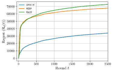
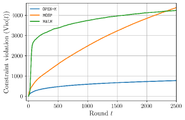
Refer to caption — Figure 1: Dynamic regret comparison of OPEN-M, MOSP and MALM

We observe sublinear dynamic regret and constraint violation from all three algorithms illustrating they are well-adapted to this problem. We remark that OPEN-M exhibits a lower regret than both the MOSP and MALM algorithms. Indeed, the dynamic regret of OPEN-M is an order of magnitude smaller. OPEN-M also has significantly better constraint violation compared to the other two algorithms.

5 Conclusion

In this paper, a second-order approach for online constrained optimization is developed. Under linear time-varying equality constraints, the resulting algorithm, OPEN-M, achieves simultaneous $O(V_{T}+1)$ dynamic regret and constraint violation bounds. These bounds are the tightest yet presented in the literature. A numerical network flow example is presented to showcase the performance of OPEN-M compared to other methods from the literature.

Considering the prevalence of interior-point methods in the offline optimization literature, an extension of the equality-constrained Newton’s method which admits inequality constraints [19], a similar extension can be envisioned for OPEN-M. A second-order approach to an online optimization problem with time-varying inequalities has the potential to improve current dynamic regret and constraint violation bounds.

References

[1] S. Shalev-Shwartz, “Online learning and online convex optimization,” Foundations and Trends® in Machine Learning, vol. 4, no. 2, pp. 107–194, 2012.
[2] M. Zinkevich, “Online convex programming and generalized infinitesimal gradient ascent,” in Proceedings of the 20th international conference on machine learning (ICML-03), 2003, pp. 928–936.
[3] J. A. Taylor, S. V. Dhople, and D. S. Callaway, “Power systems without fuel,” Renewable and Sustainable Energy Reviews, vol. 57, pp. 1322–1336, 2016.
[4] E. Hazan, “Introduction to online convex optimization,” Foundations and Trends® in Machine Learning, vol. 2, no. 3-4, pp. 157–325, 2015.
[5] F. Badal, S. Sarker, and S. Das, “A survey on control issues in renewable energy integration and microgrid,” Protection and Control of Modern Power Systems, vol. 4, no. 1, 2019.
[6] T. Chen, Q. Ling, and G. B. Giannakis, “An online convex optimization approach to proactive network resource allocation,” IEEE Transactions on Signal Processing, vol. 65, pp. 6350–6364, 2017.
[7] H. Yu and M. J. Neely, “A low complexity algorithm with O( $\sqrt{T}$ ) regret and O(1) constraint violations for online convex optimization with long term constraints,” Journal of Machine Learning Research, vol. 21, no. 1, pp. 1–24, 2020.
[8] D. J. Leith and G. Iosifidis, “Penalised FTRL with time-varying constraints,” arXiv preprint arXiv:2204.02197, 2022.
[9] J. D. Abernethy, E. Hazan, and A. Rakhlin, “Interior-point methods for full-information and bandit online learning,” IEEE Transactions on Information Theory, vol. 58, no. 7, pp. 4164–4175, 2012.
[10] M. J. Neely and H. Yu, “Online convex optimization with time-varying constraints,” 2017.
[11] X. Cao and K. J. Liu, “Online convex optimization with time-varying constraints and bandit feedback,” IEEE Transactions on Automatic Control, vol. 64, pp. 2665–2680, 2018.
[12] H. Liu, X. Xiao, and L. Zhang, “Augmented langragian methods for time-varying constrained online convex optimization,” arXiv preprint arXiv:2205.09571, 2022.
[13] A. Lesage-Landry, H. Wang, I. Shames, P. Mancarella, and J. A. Taylor, “Online convex optimization of multi-energy building-to-grid ancillary services,” IEEE Trans. on Control Syst. Technol., 2019.
[14] Q. Liu, W. Wu, L. Huang, and Z. Fang, “Simultaneously achieving sublinear regret and constraint violations for online convex optimization with time-varying constraints,” Performance Evaluation, vol. 152, 2021.
[15] J. Mulvaney-Kemp, S. Park, M. Jin, and J. Lavaei, “Dynamic regret bounds for constrained online nonconvex optimization based on Polyak-Lojasiewicz regions,” IEEE Transactions on Control of Network Systems, pp. 1 – 12, 2022.
[16] M. Fazlyab, S. Paternain, V. M. Preciado, and A. Ribeiro, “Prediction-correction interior-point method for time-varying convex optimization,” IEEE Transactions on Automatic Control, vol. 63, no. 7, pp. 1973–1986, 2018.
[17] A. Lesage-Landry, J. A. Taylor, and I. Shames, “Second-order online nonconvex optimization,” IEEE Transactions on Automatic Control, vol. 66, no. 10, pp. 4866–4872, 2021.
[18] S. Boyd and L. Vandenberghe, Convex Optimization. Cambridge University Press, 2004.
[19] J. Renegar, A Mathematical View of Interior-Point Methods in Convex Optimization. Society for Industrial and Applied Mathematics, 2001.
[20] R. Ahuja, T. Magnanti, and J. Orlin, Network Flows Theory, Algorithms and Applications. Prentice-Hall, 1993.
[21] P. Nardelli, N. Rubido, C. Wang, M. Baptista, C. Pomalaza-Raez, P. Cardieri, and M. Latva-aho., “Models for the modern power grid,” The European Physical Journal Special Topics, vol. 223, 2014.

	$\displaystyle\left\lVert\nabla^{2}\tilde{f_{t}}(\mathbf{z})-\nabla^{2}\tilde{f_{t}}(\mathbf{z}_{t}^{*})\right\rVert$	$\displaystyle=\big{\\|}\mathbf{F}_{t}\big{(}\nabla^{2}f_{t}(\mathbf{F}_{t}\mathbf{z}+\mathbf{\hat{x}})-$
		$\displaystyle\quad\quad\quad\nabla^{2}f_{t}(\mathbf{F}_{t}\mathbf{z}^{*}_{t}+\mathbf{\hat{x}})\big{)}\mathbf{F}_{t}^{\top}\big{\\|}$
		$\displaystyle\leq\left\lVert\mathbf{F}_{t}\right\rVert^{2}\big{\\|}\nabla^{2}f_{t}(\mathbf{F}_{t}\mathbf{z}+\mathbf{\hat{x}})-$
		$\displaystyle\quad\quad\quad\quad\nabla^{2}f_{t}(\mathbf{F}_{t}\mathbf{z}^{*}_{t}+\mathbf{\hat{x}})\big{\\|}$
		$\displaystyle\leq\left\lVert\mathbf{F}_{t}\right\rVert^{2}L\left\lVert\mathbf{F}_{t}(\mathbf{z}-\mathbf{z}^{*}_{t})\right\rVert$
		$\displaystyle\leq L\left\lVert\mathbf{F}_{t}\right\rVert^{3}\left\lVert\mathbf{z}-\mathbf{z}^{*}_{t}\right\rVert,$