This paper was converted on www.awesomepapers.org from LaTeX by an anonymous user.
Want to know more? Visit the Converter page.

An Optimal Transport approach to arbitrage correction: Application to volatility Stress-Tests

Marius Chevallier1,2    Stefano De Marco1    Pierre-Emmanuel Lévy-dit-Vehel2
(January 20, 2025)
Abstract

We present a method based on optimal transport to remove arbitrage opportunities within a finite set of option prices. The method is notably intended for regulatory stress-tests, which impose to apply important local distortions to implied volatility surfaces. The resulting stressed option prices are naturally associated to a family of signed marginal measures: we formulate the process of removing arbitrage as a projection onto the subset of martingale measures with respect to a Wasserstein metric in the space of signed measures. We show how this projection problem can be recast as an optimal transport problem; in view of the numerical solution, we apply an entropic regularization technique. For the regularized problem, we derive a strong duality formula, show convergence results as the regularization parameter approaches zero, and formulate a multi-constrained Sinkhorn algorithm, where each iteration involves, at worse, finding the root of an explicit scalar function. The convergence of this algorithm is also established. We compare our method with the existing approach by [Cohen, Reisinger and Wang, Appl. Math. Fin. 2020] across various scenarios and test cases.

1CMAP, Ecole Polytechnique, Institut Polytechnique de Paris
2Société Générale, Global Risk Methodologies111This work was carried out as part of a collaboration (thèse CIFRE) between CMAP and Société Générale. The findings and conclusions presented in this paper are solely those of the authors and do not represent the views of Société Générale. Contact author: Marius Chevallier, marius.chevallier@polytechnique.edu.
Acknowledgments: we thank Ghislain Essome-Boma, Quentin Jacquemart, Laurent Jullien, Claude Martini, Mohamed Sbai, Fabien Thiery, and Justine Yedikardachian for stimulating discussions and useful insights.


Keywords: Arbitrage, Volatility Stress-Tests, Optimal Transport, Entropic Regularization, Sinkhorn Algorithm.
Mathematics Subject Classification: 91G80, 49Q22.
JEL Classification: C18, C61, C65.

1 Introduction

In order to steer their risk/reward profile and maintain sufficient capital to face crises, financial institutions frequently compute several metrics to monitor the risks inherent to their activities. Among these risks, market risk refers to potential losses induced by market moves on the income of trading activities. Assessing market risk, besides being mandatory to compute regulatory capital requirements, is key to manage the activities of the front office. For instance, the Value-at-Risk (a quantile of the global short-term Profit-and-Loss or P&L) is a metric generally evaluated on a daily basis that helps firms identify trading desks that are the most at risk and thus steer their business. The computation of VaR, as for many other metrics, requires to generate scenarios for risk factors, i.e. quantities which determine the values of financial instruments (equity index levels, commodity prices, interest rates…). A fundamental risk factor that drives options values is the implied volatility surface (IVS). In order to estimate market risk carried by option portfolios, it is common for financial institutions to apply some stress-tests directly to the IVS (so to tailor design risky scenarios). This practice is even compulsory within the Fundamental Review of the Trading Book (FRTB), the most recent international regulation supervising minimum capital requirements for market risk (see [3], or Article 9 in [21]). However, from a modeling point of view, the IVS has shape constraints induced by the no-arbitrage assumptions. Stress testing often involves applying local deformations which may result in an IVS that does not fulfill these constraints, preventing the pricing functions of the institution from yielding meaningful results, especially on exotic products that rely on a global calibration. It is often a challenge for the industry to be compliant with both the regulation and a sound mathematical framework. In this paper, we investigate this problem and propose a novel approach to construct a solution.

1.1 Literature review

1.1.1 Detection and removal of arbitrage

An arbitrage opportunity is a trading strategy that has zero cost and a positive probability of making profit. A static arbitrage relates to a strategy consisting in fixed positions taken at present time on available assets (options and underlying), with the possibility to adjust the position on the underlying a finite number of times in the future (a situation often referred to as semi-static). Other arbitrages are called dynamic arbitrages. Carr & Madan [10] provided sufficient conditions to ensure absence of static arbitrages in a set of option prices on a rectangular grid, composed of a finite number of maturities, but countably many strikes. Davis and Hobson [17] extended their work to a more realistic framework, with a rectangular grid defined by a finite set of maturities and strikes. Cousot [14, 15] formulated a more general result for a finite but non-rectangular grid (even with solely bid/ask information), which corresponds to the real case in equity markets, where different strikes are typically quoted for different maturities. All these works formulate numerical tests to apply to a given set of option prices in order to check for the existence of a martingale process fitting those option prices, which is equivalent to no-arbitrage according to the First Fundamental Theorem of Asset Pricing. More recently, Cohen et al. [13], building on the aforementioned works, have formulated an algorithm to remove arbitrages from option price data (“arbitrage repair”) under the form of a linear program, with the possibility to use bid/ask prices as soft bounds. Removing arbitrages may also be addressed with smoothing techniques, which basically consist in fitting an arbitrage-free model to the data, by minimizing some criterion (see [22] for example).

Link with signed measures. While classical results link no-arbitrage with the existence of probability (hence positive) measures, a signed measure can be naturally associated (in the usual way, actually) to option prices with arbitrages, and this will be the starting point of our analysis. Concerning related literature, we note that Jarrow and Madan [25] extended the Second Fundamental Theorem of Asset Pricing to the case of an economy with infinitely many assets and where arbitrages may occur, establishing the equivalence between a certain notion of market completeness and the uniqueness of an equivalent signed local martingale measure.

1.1.2 Optimal Transport and applications to finance

The theory of optimal transport (OT) initiated by Monge and Kantorovitch (see the monographs [33, 34] for an extensive description of the theory and some of its applications) has been used to define metrics of Wasserstein-type between signed measures. Piccoli et al. [28] defined a Wasserstein norm on the space of finite signed measures on d\mathbb{R}^{d}, relying on distances between unbalanced positive measures. They used it to prove well-posedness of a non-local transport equation with a source term given by a signed measure. Ambrosio et al. [2] give another definition, in the context of superconductivity modeling. We will use the latter to formulate the correction of arbitrage in option prices as a projection problem of a signed measure onto the subset of martingale measures. Wasserstein projections of probability measures have of course been considered in a variety of fields; in the context of finance, Alfonsi et al. [1] consider projections with respect to the usual ϱ\varrho-Wasserstein distance (ϱ1\varrho\geq 1) as a tool to sample the marginal laws of a stochastic process while respecting the convex order condition, with a view on the numerical solvability of martingale optimal transport problems. In its turn, martingale optimal transport in finance was introduced by [5] with another goal, namely to derive model-independent bounds and hedging strategies for exotic options. Recently, another aspect of optimal transport was used in [35], where the author proposes to find suitable Monge maps that preserve convex order as a tool for data generation without arbitrage.

1.1.3 Entropic optimal transport and Sinkhorn’s algorithm

A popular method used in numerical OT is to penalize the cost functional involved in the minimization problem (the Wasserstein distance in our case) by an entropic term. This gives rise to the so-called entropic optimal transport (EOT) problem, which has gained much interest since the work of Cuturi [16], which allows for quick approximate numerical solutions. Cuturi’s solution is based on the renowned Sinkhorn’s algorithm [31], which consists of iterative projections on the marginal constraints (see [27] for a rich overview). Contrary to classical OT where the cost is linear, EOT is equivalent to minimizing a strictly convex functional known as the Kullback-Leibler divergence, or relative entropy. After the advent of EOT, extensions of Sinkhorn’s algorithm were designed to solve martingale optimal transport problems in finance [18, 19, 24, 7]. The projection approach we rely on to remove arbitrage can also be tackled with entropic regularization. Inspired by recent works of Benamou et al. [6] and Chizat et al. [12], we will formulate a “multi-constrained Sinkhorn” algorithm that incorporates more constraints than the usual ones in OT theory (i.e. the marginal constraints). Entropic projections (that is, the minimization of a relative entropy objective) have been exploited by De March and Henry-Labordère [19] as a tool to construct non-parametric fits of implied volatility smiles. Postponing precise definitions and discussions, let us point out a structural difference of our problem with theirs: [19] consider the projection of a given parametric model onto the set of martingale measures that fit some implied volatility market data. In this setting, the starting point (the probabilistic model) is arbitrage-free by construction, and, on the other side, one has to assume that the target market data satisfy the no-arbitrage condition; the whole operation takes place, then, within a set of probability measures. In our case, our starting point is an arbitrageable stressed smile (for which we know that the arbitrage condition is, in general, not satisfied) and the target is a martingale measure which is not required to fit market quotes — our main goal is precisely the creation of new data after the arbitrage removal. The mathematical framework of metric spaces of signed measures, which is the natural environment for our results and numerical methods, is therefore absent from [19].

1.2 Content of the article and our contributions

As addressed above, in this work we propose a new method based on OT to remove arbitrage from option data. In Section 2, we show how we can associate a discrete signed measure to option prices affected by arbitrage. In Section 3, we recall the concepts and results from OT that we use to define a Wasserstein metric between signed measures, following the notion already introduced in Ambrosio et al. [2]. Then, in Section 4, we define subsets of martingales in the space of discrete signed measures. Using the previously defined metric, we give the statement of our problem: the correction of arbitrage as a projection of the signed measure defined in Section 2 onto the martingale subsets. Next, we show that this problem is equivalent to an OT problem (i.e. a linear program on couplings). Section 5 is devoted to the entropic regularization of the minimization problem. We provide several results: we prove strong duality, dual attainment, and convergence when the regularization parameter tends to zero. In Section 6, we propose a multi-constrained Sinkhorn algorithm to approximate the solution of the regularized problem, for which we establish convergence as the number of iterates becomes large. The steps of the algorithm are either explicit, or boil down to finding the root of an explicit scalar function. Finally, Section 7 gathers several numerical applications to, first, showcase the theoretical results of convergence and, second, to illustrate the correction of stressed implied volatility smiles obtained with our method.

2 Setting and notations

We consider a finite set of call options written on the same underlying designated by SS. StS_{t} will stand for the value of SS at time tt. Present time is t=0t=0. The options can have different maturities 0<T1<<Tm0<T_{1}<\cdots<T_{m}. For a given maturity TiT_{i}, available strikes are denoted by 0<K1i<<Knii0<K_{1}^{i}<\cdots<K_{n_{i}}^{i}. Hence, the grid we are interested in may not be rectangular. The current price (i.e. at time 0) of the option paying (STiKji)+\left(S_{T_{i}}-K_{j}^{i}\right)^{+} at time TiT_{i} is CjiC_{j}^{i} which we assume to be positive. We suppose that interest rates and dividends paid by SS are deterministic. We denote by DiD_{i} the discount factor associated to the maturity TiT_{i} and FiF_{i} will stand for the TiT_{i}-forward price of SS at time 0. In the following, we will work with the normalized quantities Mi=STiFiM_{i}=\frac{S_{T_{i}}}{F_{i}}, kji=KjiFik_{j}^{i}=\frac{K_{j}^{i}}{F_{i}} and cji=CjiFiDic_{j}^{i}=\frac{C_{j}^{i}}{F_{i}D_{i}}. The vector of normalized prices is c=(c11,,cji,,cnmm)i=1mnic=\left(c_{1}^{1},\cdots,c_{j}^{i},\cdots,c_{n_{m}}^{m}\right)\in\mathbb{R}^{\sum_{i=1}^{m}n_{i}}.

2.1 Checking for arbitrages

The feasibility to build a consistent martingale model can be checked with model-independent tests, relying only on the available data (kji,cji)1im, 1jni\left(k_{j}^{i},c_{j}^{i}\right)_{1\leq i\leq m,\,1\leq j\leq n_{i}} (see [14, 15] for the construction of a discrete model or [19] for a continuous model). This is equivalent to no-arbitrage by the First Fundamental Theorem of Asset Pricing. Cohen et al. showed (see [13, Section 2.4, Proposition 2]) that these tests boil down to verify that cc solves a linear system of inequalities: 𝐀c𝐛\mathbf{A}c\leq\mathbf{b} with 𝐀R×i=1mni,𝐛R\mathbf{A}\in\mathbb{R}^{R\times\sum_{i=1}^{m}n_{i}},\,\mathbf{b}\in\mathbb{R}^{R}111See their github repository: https://github.com/vicaws/arbitragerepair for an implementation of 𝐀\mathbf{A} and 𝐛\mathbf{b} given arbitrary data.. If any inequality of the system is violated, then there is at least one (static) arbitrage in the data.

Cousot’s construction [14, 15] is based on the notion of convex order between marginals.

Definition 2.1.1 (Convex order).

Let mm\in\mathbb{N}^{*} and (μi)1im\left(\mu_{i}\right)_{1\leq i\leq m} be a family of probability measures on (,())(\mathbb{R},\mathcal{B}(\mathbb{R})), with finite moment of order 1. We say that (μi)1im\left(\mu_{i}\right)_{1\leq i\leq m} is non-decreasing in the convex order (NDCO) if for all convex functions f:f:\mathbb{R}\rightarrow\mathbb{R} with linear growth and for all 1iim1\leq i\leq i^{\prime}\leq m, one has

f𝑑μif𝑑μi.\int fd\mu_{i}\leq\int fd\mu_{i^{\prime}}\,.

Being NDCO is in fact a necessary and sufficient condition for the existence of a martingale μ\mu, on the product space (m,(m))\left(\mathbb{R}^{m},\mathcal{B}(\mathbb{R}^{m})\right), with marginals (μi)1im\left(\mu_{i}\right)_{1\leq i\leq m} (see Strassen’s Theorem [32]).

Let us briefly emphasize Cousot’s procedure to build discrete marginals, NDCO and consistent with the data (assuming the tests mentioned above are passed). First, we need to artificially extend the (normalized) data with two more prices at each maturity: for all i1,mi\in\llbracket 1,m\rrbracket, c0i:=1c_{0}^{i}:=1 at strike k0i:=0k_{0}^{i}:=0 and cni+1i=0c_{n_{i}+1}^{i}=0 at a strike kni+1i>kniik_{n_{i}+1}^{i}>k_{n_{i}}^{i} carefully chosen (see [14, Section 4.2]). Note that it is possible to choose kni+1i=kmaxk_{n_{i}+1}^{i}=k_{\mathrm{max}} for all i1,mi\in\llbracket 1,m\rrbracket (see Lemma 4.1.2 for more details). Then, the (normalized) call pricing function πi:kπi(k)\pi_{i}:k\mapsto\pi_{i}(k), for the maturity TiT_{i}, is defined as the decreasing and piecewise-affine function drawn by the lower boundary of the convex hull of the points {(kji,cji)|ii, 0jni+1}\left\{(k_{j}^{i^{\prime}},c_{j}^{i^{\prime}})\,|\,i\leq i^{\prime},\,0\leq j\leq n_{i^{\prime}}+1\right\} (and zero after kmaxk_{\mathrm{max}}). Under the no-arbitrage assumption, πi\pi_{i} verifies πi(kji)=cji\pi_{i}(k_{j}^{i})=c_{j}^{i} for all i,j1,m×1,nii,j\in\llbracket 1,m\rrbracket\times\llbracket 1,n_{i}\rrbracket. Furthermore, it defines a discrete probability measure μi\mu_{i}, the second derivative of πi\pi_{i} in the sense of distributions, supported on a subset of i=1m{k1i,,knii}{0,kmax}\bigcup\limits_{i=1}^{m}\left\{k_{1}^{i},\cdots,k_{n_{i}}^{i}\right\}\cup\left\{0,k_{\mathrm{max}}\right\}, satisfying πi(k)=(xk)+𝑑μi\pi_{i}(k)=\int(x-k)^{+}d\mu_{i}, for all k+k\in\mathbb{R}^{+} (see [14, Lemma 3.1]). Thus defined, the probability measures (μi)1im\left(\mu_{i}\right)_{1\leq i\leq m} are NDCO and their support is included in

Θ=i=1m{k1i,,knii}{0,kmax},\Theta=\bigcup\limits_{i=1}^{m}\left\{k_{1}^{i},\cdots,k_{n_{i}}^{i}\right\}\cup\left\{0,k_{\mathrm{max}}\right\}\,,

the collection of all strikes.

Remark 2.1.2.

The important fact here is that, up to a proper choice of kmaxk_{\mathrm{max}}, any system of call prices on the fixed grid (Ti,kji)1im, 1jni\left(T_{i},k_{j}^{i}\right)_{1\leq i\leq m,\,1\leq j\leq n_{i}} that has no arbitrage can be attained by a discrete martingale on the finite product space Θm\Theta^{m} (by Strassen’s Theorem). This is what motivated us to work in a discrete setting.

2.2 Signed measure associated to option prices with arbitrages

Assume now that there are some arbitrages in the data, meaning that c does not solve Cohen’s system of inequalities. For example, they may be due to a local stress-test applied to the associated IVS (initially arbitrage-free). In some applications, we will need to be able to control which part of the IVS must be preserved during the process of removing arbitrage opportunities. We denote by c¯\bar{c} any vector of arbitrage-free (normalized) prices, on an arbitrary sub-grid of (Ti,kji)1im, 1jni\left(T_{i},k_{j}^{i}\right)_{1\leq i\leq m,\,1\leq j\leq n_{i}}. For instance, c¯\bar{c} could correspond to the prices that were not impacted by the hypothetical stress-test mentioned above. On the contrary, it could also consist of the ones that were actually impacted, as long as, ignoring the rest of the data, they are arbitrage-free. In order to identify the maturities and the (normalized) strikes of the sub-grid, we introduce 1,m\mathcal{I}\subset\llbracket 1,m\rrbracket and for any ii\in\mathcal{I}, 𝒥i={j1<<jn¯i}{1,,ni}\mathcal{J}_{i}=\left\{j_{1}<\cdots<j_{\bar{n}_{i}}\right\}\subset\left\{1,\cdots,n_{i}\right\}, so that c¯=(c¯ji)i,j𝒥i\bar{c}=\left(\bar{c}_{j}^{i}\right)_{i\in\mathcal{I},\,j\in\mathcal{J}_{i}}. Finally, we call n¯=in¯i\bar{n}=\sum\limits_{i\in\mathcal{I}}\bar{n}_{i} the length of c¯\bar{c}.

Even if there are arbitrages, we will see that it is still possible to associate discrete measures that are consistent with the data, through a simple adaptation of Cousot’s construction. However, the resulting measures might be signed or fail to be NDCO. Similarly, we can enlarge the data with additional prices for each TiT_{i}: c0i:=1c_{0}^{i}:=1 at k0i:=0k_{0}^{i}:=0 and cni+1i:=0c_{n_{i}+1}^{i}:=0 at kni+1i=kmax>kniik_{n_{i}+1}^{i}=k_{\mathrm{max}}>k_{n_{i}}^{i} (see Lemma 4.1.2 to see how kmaxk_{\mathrm{max}} should be chosen). As previously, we call Θ\Theta the collection of all strikes, namely Θ=i=1m{k1i,,knii}{0,kmax}\Theta=\bigcup\limits_{i=1}^{m}\left\{k_{1}^{i},\cdots,k_{n_{i}}^{i}\right\}\cup\left\{0,k_{\mathrm{max}}\right\} and, to ease notations, we rewrite it as {k1,,kl}\{k_{1},\cdots,k_{l}\}, with k1<<klk_{1}<\cdots<k_{l}, so that l=#Θl=\#\Theta, k1=0k_{1}=0 and kl=kmaxk_{l}=k_{\mathrm{max}}.

Definition 2.2.1 (Signed marginal).

For a given maturity TiT_{i}, we define the discrete (signed) measure νi\nu_{i} by

νi=j=0ni+1wjδkji,\nu_{i}=\sum_{j=0}^{n_{i}+1}w_{j}\delta_{k_{j}^{i}}\,,

where δx\delta_{x} is the Dirac mass located at xx\in\mathbb{R} and

w0=1+c0ic1ik0ik1i,wj=cj+1icjikj+1ikjicjicj1ikjikj1i , 1jni,wni+1=cni+1icniikni+1iknii.\begin{array}[]{l}w_{0}=1+\frac{c_{0}^{i}-c_{1}^{i}}{k_{0}^{i}-k_{1}^{i}}\,,\\[10.0pt] w_{j}=\frac{c_{j+1}^{i}-c_{j}^{i}}{k_{j+1}^{i}-k_{j}^{i}}-\frac{c_{j}^{i}-c_{j-1}^{i}}{k_{j}^{i}-k_{j-1}^{i}}\text{ , }1\leq j\leq n_{i}\,,\\[10.0pt] w_{n_{i}+1}=-\frac{c_{n_{i}+1}^{i}-c_{n_{i}}^{i}}{k_{n_{i}+1}^{i}-k_{n_{i}}^{i}}\,.\end{array}
Remark 2.2.2.

The νi\nu_{i}’s are always well defined and have a total mass of 11. Even though they can be true probability measures (in the case of calendar arbitrages only), we still use the terminology “signed” to emphasize that they are associated to some inconsistent data.

Definition 2.2.3 (Piecewise-affine continuous pricing function).

For a fixed TiT_{i}, we define πi:+\pi_{i}:\mathbb{R}^{+}\rightarrow\mathbb{R} by

πi(k)={cj+1icjikj+1ikji(kkji)+cji if k[kji,kj+1i[0 if kkmax.\pi_{i}(k)=\left\{\begin{array}[]{ll}\frac{c_{j+1}^{i}-c_{j}^{i}}{k_{j+1}^{i}-k_{j}^{i}}(k-k_{j}^{i})+c_{j}^{i}&\text{ if }k\in\left[k_{j}^{i},k_{j+1}^{i}\right[\\ 0&\text{ if }k\geq k_{\mathrm{max}}\end{array}\right.\,.

By construction, πi\pi_{i} is piecewise-affine, continuous and πi(kji)=cji\pi_{i}(k_{j}^{i})=c_{j}^{i}.

Lemma 2.2.4 (Lemma 3.1 [14]).

For all i1,mi\in\llbracket 1,m\rrbracket and for all k+k\in\mathbb{R}^{+}, we have

(xk)+𝑑νi=πi(k).\int(x-k)^{+}d\nu_{i}=\pi_{i}(k)\,.
Remark 2.2.5.

Lemma 2.2.4 justifies why we allow ourself to employ the terminology “marginals” for the νi\nu_{i}’s, though they can be signed. Indeed, they sum up to one and calibrate the data with arbitrages.

Note that each νi\nu_{i} has a finite support included in {k1i,,knii}{0,kmax}\{k_{1}^{i},\cdots,k_{n_{i}}^{i}\}\cup\{0,k_{\mathrm{max}}\}, but can be seen as a measure distributed on Θ\Theta, with zero weights for the elements of Θ\Theta that are not in its support. The νi\nu_{i}’s being specified, we can define what we call a “joint signed measure” ν\nu, on the finite product space Θm\Theta^{m}, with marginals (νi)1im\left(\nu_{i}\right)_{1\leq i\leq m}. A simple choice would be to set ν=ν1νm\nu=\nu_{1}\otimes\cdots\otimes\nu_{m}, but this could be somehow unsatisfactory, for reasons that will become clearer in Section 4.2. From now, we just assume that ν\nu is built. Note that it satisfies ν(Θm)=1\nu(\Theta^{m})=1. In the following section, we will define a distance between signed measures with total mass equal to one, to formulate the correction of arbitrages as the projection of ν\nu onto the subset of martingales. Just recall that, from Remark 2.1.2, it is sufficient to look for martingales on Θm\Theta^{m} to get rid of arbitrages in the data (up to a choice of kmaxk_{\mathrm{max}}).

3 Distance of Wasserstein-type between signed measures

In this part, we work with a Polish space (𝒳,d)(\mathcal{X},d), and we endow it with its Borel σ\sigma-algebra, denoted by (𝒳)\mathcal{B}(\mathcal{X}). ={ν:(𝒳)|ν()=0,ν is σ-additive}\mathcal{M}=\left\{\nu:\mathcal{B}(\mathcal{X})\rightarrow\mathbb{R}\,|\,\nu(\emptyset)=0,\,\nu\text{ is }\sigma\text{-additive}\right\} is the set of finite signed measures on 𝒳\mathcal{X}. +\mathcal{M}_{+} is the subset of \mathcal{M} consisting of all finite positive measures on 𝒳\mathcal{X}. We recall that any element ν\nu of \mathcal{M} admits a unique decomposition (νJ+,νJ)(\nu_{J}^{+},\nu_{J}^{-}) (the so-called Jordan decomposition) with νJ+,νJ+\nu_{J}^{+},\nu_{J}^{-}\in\mathcal{M}_{+}, such that ν=νJ+νJ\nu=\nu_{J}^{+}-\nu_{J}^{-} and νJ+νJ\nu_{J}^{+}\perp\nu_{J}^{-}. However, note that there are infinitely many decompositions of ν\nu of the form ν=ν+ν\nu=\nu^{+}-\nu^{-}. For instance, ν+=νJ++σ\nu^{+}=\nu^{+}_{J}+\sigma and ν=νJ+σ\nu^{-}=\nu^{-}_{J}+\sigma with σ+\sigma\in\mathcal{M}_{+} is one of them. The variation of ν\nu\in\mathcal{M} is |ν|=νJ++νJ|\nu|=\nu_{J}^{+}+\nu_{J}^{-} (it is an element of +\mathcal{M}_{+}). For ϱ[1,+[\varrho\in[1,+\infty[, we also define ϱ={ν|d(x0,x)ϱd|ν|<+ for all x0𝒳}\mathcal{M}^{\varrho}=\left\{\nu\in\mathcal{M}\,|\,\int d(x_{0},x)^{\varrho}d|\nu|<+\infty\text{ for all }x_{0}\in\mathcal{X}\right\} and +ϱ=ϱ+\mathcal{M}_{+}^{\varrho}=\mathcal{M}^{\varrho}\cap\mathcal{M}_{+}. Finally, for α\alpha\in\mathbb{R}, we denote by (α)\mathcal{M}(\alpha) the set {ν|ν(𝒳)=α}\left\{\nu\in\mathcal{M}\,|\,\nu(\mathcal{X})=\alpha\right\} (and similarly ϱ(α),+(α),+ϱ(α)\mathcal{M}^{\varrho}(\alpha),\mathcal{M}_{+}(\alpha),\mathcal{M}_{+}^{\varrho}(\alpha), with obviously +(α)=+ϱ(α)=\mathcal{M}_{+}(\alpha)=\mathcal{M}_{+}^{\varrho}(\alpha)=\emptyset whenever α<0\alpha<0).

3.1 Wasserstein distances for positive measures with finite mass

Wasserstein distances are usually defined for elements in +ϱ(1)\mathcal{M}_{+}^{\varrho}(1) i.e. for probability measures with finite moment of order ϱ\varrho (see the monographs [33, 34] for more details), but it extends naturally for positive measures with some fixed finite mass α+\alpha\in\mathbb{R}_{+}^{*}. Their definition is based on the theory of optimal transport.

Definition 3.1.1 (Transference plan).

Let α+\alpha\in\mathbb{R}_{+}^{*} and μ,ν+(α)\mu,\nu\in\mathcal{M}_{+}(\alpha). A transference plan between μ\mu and ν\nu is a positive measure π\pi, on the product space 𝒳×𝒳\mathcal{X}\times\mathcal{X}, that satisfies

π(A×𝒳)=μ(A),π(𝒳×B)=ν(B),\pi(A\times\mathcal{X})=\mu(A),\;\pi(\mathcal{X}\times B)=\nu(B)\,,

for all A,B(𝒳)A,B\in\mathcal{B}(\mathcal{X}).

The set of transference plans is denoted by Γ(μ,ν)\Gamma(\mu,\nu). We shall also refer to it as the set of couplings between μ\mu and ν\nu.

Definition 3.1.2 (Wasserstein distance of order ϱ\varrho).

Let α+\alpha\in\mathbb{R}_{+}^{*}, ϱ[1,+[\varrho\in[1,+\infty[ and μ,ν+ϱ(α)\mu,\nu\in\mathcal{M}_{+}^{\varrho}(\alpha). The Wasserstein distance of order ϱ\varrho between μ\mu and ν\nu is defined by

Wϱ(μ,ν)=(infπΓ(μ,ν)d(x,y)ϱ𝑑π)1ϱ.W_{\varrho}(\mu,\nu)=\left(\underset{\pi\in\Gamma(\mu,\nu)}{\inf}\,\int d(x,y)^{\varrho}d\pi\right)^{\frac{1}{\varrho}}.
Theorem 3.1.3 (See Theorem 7.3 in [33] for α=1\alpha=1).

For any ϱ[1,+[\varrho\in[1,+\infty[, and any α+\alpha\in\mathbb{R}_{+}^{*}, the space (+ϱ(α),Wϱ)\left(\mathcal{M}_{+}^{\varrho}(\alpha),W_{\varrho}\right) is a metric space.

Theorem 3.1.4 (Kantorovich-Rubinstein duality formula, see [33] for the case α=1\alpha=1).

Let α+\alpha\in\mathbb{R}_{+}^{*} and μ,ν+1(α)\mu,\nu\in\mathcal{M}_{+}^{1}(\alpha). Then,

W1(μ,ν)=supφLip(𝒳),φLip1𝒳φd(μν),W_{1}(\mu,\nu)=\underset{\varphi\in\mathrm{Lip}\left(\mathcal{X}\right),\,||\varphi||_{\mathrm{Lip}}\leq 1}{\sup}\;\int_{\mathcal{X}}\varphi\,d(\mu-\nu)\,,

where Lip(𝒳)\mathrm{Lip}\left(\mathcal{X}\right) is the set of Lipschitz functions on 𝒳\mathcal{X} and φLip:=supx,y𝒳|φ(x)φ(y)|d(x,y)||\varphi||_{\mathrm{Lip}}:=\underset{x,y\in\mathcal{X}}{\sup}\;\frac{|\varphi(x)-\varphi(y)|}{d(x,y)}.

3.2 A Wasserstein distance between signed measures

The following definition, motivated by Ambrosio et al. [2], extends the 11-Wasserstein distance to signed measures.

Definition 3.2.1 (Wasserstein distance between signed measures with unit mass).

Let μ\mu and ν\nu be two elements of 1(1)\mathcal{M}^{1}(1). The Wasserstein distance between μ\mu and ν\nu is defined by

𝕎1(μ,ν)=W1(μ++ν,μ+ν+),\mathbb{W}_{1}(\mu,\nu)=W_{1}(\mu^{+}+\nu^{-},\mu^{-}+\nu^{+})\,,

for any decomposition μ+,μ+1\mu^{+},\mu^{-}\in\mathcal{M}_{+}^{1} and ν+,ν+1\nu^{+},\nu^{-}\in\mathcal{M}_{+}^{1} of μ\mu and ν\nu.

Proposition 3.2.2.

𝕎1\mathbb{W}_{1} is a well-defined functional. Moreover, we have the following duality formula

𝕎1(μ,ν)=supφLip(𝒳),φLip1𝒳φd(μν).\mathbb{W}_{1}(\mu,\nu)=\underset{\varphi\in\mathrm{Lip}\left(\mathcal{X}\right),\,||\varphi||_{\mathrm{Lip}}\leq 1}{\sup}\;\int_{\mathcal{X}}\varphi\,d(\mu-\nu)\,.
Proof.

Let μ,ν1(1)\mu,\nu\in\mathcal{M}^{1}(1) and μ+,μ,ν+,ν+1\mu^{+},\mu^{-},\nu^{+},\nu^{-}\in\mathcal{M}^{1}_{+} such that μ=μ+μ\mu=\mu^{+}-\mu^{-} and ν=ν+ν\nu=\nu^{+}-\nu^{-}.

Because μ(𝒳)=ν(𝒳)=1\mu(\mathcal{X})=\nu(\mathcal{X})=1, we have μ+(𝒳)+ν(𝒳)=ν+(𝒳)+μ(𝒳)=α1\mu^{+}(\mathcal{X})+\nu^{-}(\mathcal{X})=\nu^{+}(\mathcal{X})+\mu^{-}(\mathcal{X})=\alpha\geq 1. Hence μ++ν\mu^{+}+\nu^{-} and μ+ν+\mu^{-}+\nu^{+} are elements of +1(α)\mathcal{M}^{1}_{+}(\alpha). Then, from the duality formula 3.1.4, we obtain

𝕎1(μ,ν)\displaystyle\mathbb{W}_{1}(\mu,\nu) =W1(μ++ν,μ+ν+)\displaystyle=W_{1}(\mu^{+}+\nu^{-},\mu^{-}+\nu^{+})
=supφLip(𝒳),φLip1𝒳φd((μ++ν)(μ+ν+))\displaystyle=\underset{\varphi\in\mathrm{Lip}\left(\mathcal{X}\right),\,||\varphi||_{\mathrm{Lip}}\leq 1}{\sup}\;\int_{\mathcal{X}}\varphi\,d((\mu^{+}+\nu^{-})-(\mu^{-}+\nu^{+}))
=supφLip(𝒳),φLip1𝒳φd(μν).\displaystyle=\underset{\varphi\in\mathrm{Lip}\left(\mathcal{X}\right),\,||\varphi||_{\mathrm{Lip}}\leq 1}{\sup}\;\int_{\mathcal{X}}\varphi\,d(\mu-\nu)\,.

From this duality, we see that the value of 𝕎1(μ,ν)\mathbb{W}_{1}(\mu,\nu) does not depend on the decomposition of μ\mu and ν\nu. ∎

Proposition 3.2.3.

The space (1(1),𝕎1)\left(\mathcal{M}^{1}(1),\mathbb{W}_{1}\right) is a metric space.

Proof.

From the duality in Proposition 3.2.2, 𝕎1\mathbb{W}_{1} is symmetric (with the change of variable φφ\varphi\leftarrow-\varphi). Moreover, from Definition 3.2.1, 𝕎1\mathbb{W}_{1} is non-negative, as the classical 11-Wasserstein distance is. From the positivity of W1W_{1}, we get 𝕎1(μ,ν)=0μ++ν=μ+ν+μ=ν\mathbb{W}_{1}(\mu,\nu)=0\Longleftrightarrow\mu^{+}+\nu^{-}=\mu^{-}+\nu^{+}\Longleftrightarrow\mu=\nu. Finally, for μ,ν,θ1(1)\mu,\nu,\theta\in\mathcal{M}^{1}(1), and for φLip(𝒳)\varphi\in\mathrm{Lip}\left(\mathcal{X}\right) with φLip1||\varphi||_{\mathrm{Lip}}\leq 1, we have

𝒳φd(μν)\displaystyle\int_{\mathcal{X}}\varphi\,d(\mu-\nu) =𝒳φd(μθ)+𝒳φd(θν)\displaystyle=\int_{\mathcal{X}}\varphi\,d(\mu-\theta)+\int_{\mathcal{X}}\varphi\,d(\theta-\nu)
supφLip(𝒳),φLip1𝒳φd(μθ)+supφLip(𝒳),φLip1𝒳φd(θν).\displaystyle\leq\underset{\varphi\in\mathrm{Lip}\left(\mathcal{X}\right),\,||\varphi||_{\mathrm{Lip}}\leq 1}{\sup}\;\int_{\mathcal{X}}\varphi\,d(\mu-\theta)+\underset{\varphi\in\mathrm{Lip}\left(\mathcal{X}\right),\,||\varphi||_{\mathrm{Lip}}\leq 1}{\sup}\;\int_{\mathcal{X}}\varphi\,d(\theta-\nu)\,.

Taking the supremum over all φ\varphi on the left-hand side and using Proposition 3.2.2 leads to the triangle inequality. ∎

4 Projection on subsets of martingales

Hereafter, we work with 𝒳=Θm\mathcal{X}=\Theta^{m} and dd a distance on m\mathbb{R}^{m}. In the discrete case, =ϱ\mathcal{M}=\mathcal{M}^{\varrho} and +=+ϱ\mathcal{M}_{+}=\mathcal{M}_{+}^{\varrho} for all ϱ[1,+[\varrho\in[1,+\infty[. Let NN\in\mathbb{N}^{*} be the cardinality of Θm\Theta^{m} i.e. N=lmN=l^{m}. For p1,Np\in\llbracket 1,N\rrbracket, there exists a unique mm-tuple (p1,,pm)1,lm(p_{1},\cdots,p_{m})\in\llbracket 1,l\rrbracket^{m} such that p=1+i=1m(pi1)lmip=1+\sum\limits_{i=1}^{m}(p_{i}-1)l^{m-i} (a slight reformulation of the decomposition of p1p-1 in the base ll). With this one to one correspondence, we can define the path xp=(kp1,,kpm)Θmx_{p}=\left(k_{p_{1}},\cdots,k_{p_{m}}\right)\in\Theta^{m}, identified to a vector in m\mathbb{R}^{m}, that starts at kp1k_{p_{1}} and ends up at kpmk_{p_{m}}. We denote by DD the distance matrix (d(xp,xq))1p,qN\left(d(x_{p},x_{q})\right)_{1\leq p,q\leq N}. The state space being Θm\Theta^{m} here, any element ν\nu\in\mathcal{M} can either be written as ν=p=1Nνpδxp\nu=\sum\limits_{p=1}^{N}\nu_{p}\delta_{x_{p}} or ν=1p1,,pmlνp1,,pmδ(kp1,,kpm)\nu=\sum\limits_{1\leq p_{1},\cdots,p_{m}\leq l}\nu_{p_{1},\cdots,p_{m}}\delta_{(k_{p_{1}},\cdots,k_{p_{m}})}, with νp,νp1,,pm\nu_{p},\nu_{p_{1},\cdots,p_{m}}\in\mathbb{R}. Thus, we will identify signed measures on Θm\Theta^{m} either by vectors in N\mathbb{R}^{N} or mm-rank tensors in l××l\mathbb{R}^{l\times\cdots\times l}, depending on the situation. Finally, we denote by (Mi)1im(M_{i})_{1\leq i\leq m} the canonical process: Mi:Θm(k1,,km)kiM_{i}:\Theta^{m}\ni(k_{1},\cdots,k_{m})\mapsto k_{i} and we introduce the shorthand notations (νp1,,pm):=(νp1,,pm)1p1,,pml\left(\nu_{p_{1},\cdots,p_{m}}\right):=\left(\nu_{p_{1},\cdots,p_{m}}\right)_{1\leq p_{1},\cdots,p_{m}\leq l} and p1,,pm:=1p1,,pml\sum\limits_{p_{1},\cdots,p_{m}}:=\sum\limits_{1\leq p_{1},\cdots,p_{m}\leq l}.

4.1 Subsets of interest

Definition 4.1.1 (Martingale measures on Θm\Theta^{m}).

We call \mathscr{M}\subset\mathcal{M} the subset of martingale measures centered at 11. An element μ\mu\in\mathscr{M} must satisfy

μ0,\displaystyle\mu\geq 0\,,
μ(Θm)=1,\displaystyle\mu(\Theta^{m})=1\,,
𝔼μ[M1]=1,\displaystyle\mathbb{E}^{\mu}\left[M_{1}\right]=1\,,
𝔼μ[Mi+1Mi|M1,,Mi]=0 for all i1,m1.\displaystyle\mathbb{E}^{\mu}\left[M_{i+1}-M_{i}|M_{1},\cdots,M_{i}\right]=0\text{ for all }i\in\llbracket 1,m-1\rrbracket\,.

Identifying μ\mu to a mm-rank tensor (μp1,,pm)\left(\mu_{p_{1},\cdots,p_{m}}\right), this translates equivalently to

μp1,,pm0(N inequality constraints),\displaystyle\mu_{p_{1},\cdots,p_{m}}\geq 0\;(N\text{ inequality constraints})\,, (1)
p1,,pmμp1,,pm=1(1 equality constraint),\displaystyle\sum\limits_{p_{1},\cdots,p_{m}}\mu_{p_{1},\cdots,p_{m}}=1\;(1\text{ equality constraint})\,, (2)
p1,,pmkp1μp1,,pm=1(1 equality constraint),\displaystyle\sum\limits_{p_{1},\cdots,p_{m}}k_{p_{1}}\mu_{p_{1},\cdots,p_{m}}=1\;(1\text{ equality constraint})\,, (3)
pi+1,,pm(kpi+1kpi)μp1,,pm=0,\displaystyle\sum\limits_{p_{i+1},\cdots,p_{m}}\left(k_{p_{i+1}}-k_{p_{i}}\right)\mu_{p_{1},\cdots,p_{m}}=0\,, (4)

where (4) must stand for all i1,,m1i\in\llbracket 1,\cdots,m-1\rrbracket, for all p1,,pi1,lip_{1},\cdots,p_{i}\in\llbracket 1,l\rrbracket^{i} (i=1m1li=Nll1\sum\limits_{i=1}^{m-1}l^{i}=\frac{N-l}{l-1} equality constraints).

The total number of equality constraints is L=2+Nll1L=2+\frac{N-l}{l-1}.

We also introduce c¯\mathscr{M}_{\bar{c}}, the subset of \mathscr{M}, where the elements (seen as mm-rank tensors) satisfy the additional calibration property

p1,..,pi,..,pm(kpikji)+μp1,..,pi,..,pm=c¯ji,\sum\limits_{p_{1},..,p_{i},..,p_{m}}(k_{p_{i}}-k_{j}^{i})^{+}\mu_{p_{1},..,p_{i},..,p_{m}}=\bar{c}_{j}^{i}\,, (5)

where (5) must stand for all ii\in\mathcal{I}, for all j𝒥ij\in\mathcal{J}_{i} (n¯\bar{n} equality constraints).

Therefore, an element of c¯\mathscr{M}_{\bar{c}} must satisfy L¯=L+n¯\bar{L}=L+\bar{n} equality constraints.

All these constraints are linear in the variable μ\mu. Hence, seeing now measures as vectors in N\mathbb{R}^{N}, there exists a matrix AL×NA\in\mathbb{R}^{L\times N} and a vector bLb\in\mathbb{R}^{L} (resp. a matrix A¯L¯×N\bar{A}\in\mathbb{R}^{\bar{L}\times N} and a vector b¯L¯\bar{b}\in\mathbb{R}^{\bar{L}}) such that ={μN|μ0,Aμ=b}\mathscr{M}=\left\{\mu\in\mathbb{R}^{N}\,|\,\mu\geq 0,\,A\mu=b\right\} (resp. c¯={μN|μ0,A¯μ=b¯}\mathscr{M}_{\bar{c}}=\left\{\mu\in\mathbb{R}^{N}\,|\,\mu\geq 0,\,\bar{A}\mu=\bar{b}\right\}).

Lemma 4.1.2.

If one chooses kmax>max(1,max1imknii)k_{\mathrm{max}}>\max\left(1,\,\underset{1\leq i\leq m}{\max}\,k_{n_{i}}^{i}\right), then \mathscr{M} is non-empty.

If

kmax>max(max1imknii,maxikjn¯ii2ac¯jn¯ii),k_{\mathrm{max}}>\max\left(\,\underset{1\leq i\leq m}{\max}\,k_{n_{i}}^{i},\,\underset{i\in\mathcal{I}}{\max}\,k_{j_{\bar{n}_{i}}}^{i}-\frac{2}{a}\bar{c}_{j_{\bar{n}_{i}}}^{i}\right),

with

a=max({c¯jic¯jikjikji|i,i,j𝒥i{0},j𝒥i{0}such thatkji>kji}),a=\max\,\left(\left\{\frac{\bar{c}_{j}^{i}-\bar{c}_{j^{\prime}}^{i^{\prime}}}{k_{j}^{i}-k_{j^{\prime}}^{i^{\prime}}}\,|\,i,i^{\prime}\in\mathcal{I},\,j\in\mathcal{J}_{i}\cup\{0\},\,j^{\prime}\in\mathcal{J}_{i^{\prime}}\cup\{0\}\;\text{such that}\;k_{j}^{i}>k_{j^{\prime}}^{i^{\prime}}\right\}\cap\mathbb{R}^{*}_{-}\right)\,,

then, c¯\mathscr{M}_{\bar{c}} is non-empty.

Proof.

For the first part, define μi=(11kmax)δk1+1kmaxδkmax\mu_{i}=\left(1-\frac{1}{k_{\mathrm{max}}}\right)\delta_{k_{1}}+\frac{1}{k_{\mathrm{max}}}\delta_{k_{\mathrm{max}}}, for i1,mi\in\llbracket 1,m\rrbracket. The μi\mu_{i}’s are discrete probability measures on Θ\Theta (because kmax=klk_{\mathrm{max}}=k_{l} by definition) satisfying xμi(dx)=1\int x\,\mu_{i}(dx)=1. Moreover, they are obviously NDCO because equal. From Strassen’s Theorem, there exists a martingale measure μ\mu on Θm\Theta^{m}, with these marginals, hence an element of \mathscr{M}.

The second part follows from Cousot’s construction [14] applied to the data formed by (kji,c¯ji)i,j𝒥i\left(k_{j}^{i},\bar{c}_{j}^{i}\right)_{i\in\mathcal{I},\,j\in\mathcal{J}_{i}}. We obtain probability measures (mi)i\left(m_{i}\right)_{i\in\mathcal{I}} NDCO, with support included in Θ\Theta. By construction, they satisfy xmi(dx)=1\int x\,m_{i}(dx)=1 and (xkji)+mi(dx)=c¯ji\int(x-k_{j}^{i})^{+}\,m_{i}(dx)=\bar{c}^{i}_{j}, for all ii\in\mathcal{I} and j𝒥ij\in\mathcal{J}_{i}. Then, we define

μi={mi if iminearest if i and iimaxmimax if i>imax,\mu_{i}=\left\{\begin{array}[]{l}m_{i}\text{ if }i\in\mathcal{I}\\ m_{i_{\mathrm{nearest}}}\text{ if }i\notin\mathcal{I}\text{ and }i\leq i_{\mathrm{max}}\\ m_{i_{\mathrm{max}}}\text{ if }i>i_{\mathrm{max}}\end{array}\right.\,,

with inearest=mini,iiii_{\mathrm{nearest}}=\underset{i^{\prime}\in\mathcal{I},i\leq i^{\prime}}{\min}\,i^{\prime} and imax=maxiii_{\mathrm{max}}=\underset{i^{\prime}\in\mathcal{I}}{\max}\,i^{\prime}.

Thus defined, the μi\mu_{i}’s are still NDCO so, from Strassen’s Theorem, there exists a martingale measure μ\mu on Θm\Theta^{m} with these marginals, hence an element of \mathscr{M}. As the marginals also calibrate c¯\bar{c}, μ\mu is actually an element of c¯\mathscr{M}_{\bar{c}}. ∎

For the rest of the paper, we assume that kmaxk_{\mathrm{max}} is properly chosen, so that Lemma 4.1.2 always applies.

4.2 Choice of the joint signed measure ν\nu

As discussed in 2.2, the signed marginals (νi)1im(\nu_{i})_{1\leq i\leq m} are uniquely defined in our setting. However, we have a degree of freedom in the choice of the joint signed measure ν\nu with these marginals. Even though there are arbitrages, the choice ν=ν1νm\nu=\nu_{1}\otimes\cdots\otimes\nu_{m} would correspond, in some way, to an independent framework which is unsatisfactory. Indeed, recall that our aim is to project ν\nu onto the subset of martingales. Martingales never have independent marginals (except for constant martingales). Consequently, choosing ν\nu as the product measure would be somehow “very far” from \mathscr{M} (or c¯\mathscr{M}_{\bar{c}}). Thus, we can try to build a signed measure that already looks like a martingale. We propose below a possible construction for this joint signed measure, but leave for future work the question of whether this choice can be improved.

Let us assume, for the moment, that (νi)1im(\nu_{i})_{1\leq i\leq m} are true probability measures NDCO. Then, from Strassen’s Theorem, there exists a discrete probability measure ν\nu on Θm\Theta^{m} satisfying (1), (2), (3), (4) and

pk,kiνp1,,pm=(νi)pi,\sum_{p_{k},\,k\neq i}\nu_{p_{1},\cdots,p_{m}}=\left(\nu_{i}\right)_{p_{i}}\,, (6)

for all i1,mi\in\llbracket 1,m\rrbracket, for all pi1,lp_{i}\in\llbracket 1,l\rrbracket (mlml equality constraints), where (νi)pi(\nu_{i})_{p_{i}} is the pip_{i}-th coefficient of the vector νi\nu_{i}. The constraint (6) is again linear in the variable ν=(νp1,,pm)\nu=(\nu_{p_{1},\cdots,p_{m}}). Therefore, we can write ν{xN|x0,Aνx=bν}\nu\in\left\{x\in\mathbb{R}^{N}\,|\,x\geq 0,A_{\nu}x=b_{\nu}\right\}, with Aν=[AB]A_{\nu}=\,\begin{bmatrix}A\\ B\end{bmatrix} for some Bml×NB\in\mathbb{R}^{ml\times N} and bν=(b,ν1,,νm)L+mlb_{\nu}=\left(b,\nu_{1},\cdots,\nu_{m}\right)\in\mathbb{R}^{L+ml}. However, there is some redundancy in the constraints satisfied by ν\nu. For instance, if (4) and (6) are verified, then (2) and (3) are automatically true by construction. Said differently, AνA_{\nu} doesn’t have full rank. Removing the redundant rows (resp. coefficients) in AνA_{\nu} (resp. bνb_{\nu}) and keeping the same notations for simplicity, we may assume that ν\nu belongs to {xN|x0,Aνx=bν}\left\{x\in\mathbb{R}^{N}\,|\,x\geq 0,A_{\nu}x=b_{\nu}\right\}, with AνLν×NA_{\nu}\in\mathbb{R}^{L_{\nu}\times N}, bνLνb_{\nu}\in\mathbb{R}^{L_{\nu}}, and rank(Aν)=min(Lν,N)<L+ml\mathrm{rank}(A_{\nu})=\min(L_{\nu},N)<L+ml.

From this remark and coming back to our setting, we could try to find ν\nu in the set signed={xN|Aνx=bν}\mathscr{M}_{signed}=\left\{x\in\mathbb{R}^{N}\,|\,A_{\nu}x=b_{\nu}\right\} i.e. removing the positivity constraint (otherwise this set is empty because of arbitrages). It corresponds to the set of “signed martingales”, with fixed marginals (νi)1im(\nu_{i})_{1\leq i\leq m}. Besides, recall from the positive case that the product measure maximizes the entropy, or, said differently, the randomness among joint distributions with prescribed marginals. Because the entropy is not well defined for signed measures, an alternative could be to choose a signed martingale close to ν1νm\nu_{1}\otimes\cdots\otimes\nu_{m}. To some extent, it corresponds to the least biased choice. Therefore, we choose ν\nu to be the unique solution of the following quadratic constrained optimization problem

minxsignedxν1νm2.\underset{x\in\mathscr{M}_{signed}}{\min}\;||x-\nu_{1}\otimes\cdots\otimes\nu_{m}||^{2}.

signed\mathscr{M}_{signed} is closed and non-empty because AνA_{\nu} has full rank. Moreover, ||.||2||.||^{2} is continuous and coercive, hence existence of a minimizer follows. Uniqueness comes from the strict convexity of ||.||2||.||^{2}.

ν\nu will remain fixed for the rest of the paper. We define ν+,νN\nu^{+},\nu^{-}\in\mathbb{R}^{N} by ν+=(max(νp,0))1pN\nu^{+}=\left(\max(\nu_{p},0)\right)_{1\leq p\leq N} and ν=(max(νp,0))1pN\nu^{-}=\left(\max(-\nu_{p},0)\right)_{1\leq p\leq N}. Note that we have ν0N\nu^{-}\neq 0_{\mathbb{R}^{N}}, because of the presence of arbitrages. Since μ𝕎1(μ,ν)\mu\mapsto\mathbb{W}_{1}(\mu,\nu) does not depend on the decomposition of ν\nu (see Proposition 3.2.2), we may add the same positive vector to ν+\nu^{+} and ν\nu^{-}, to obtain a positive decomposition of ν\nu. Keeping the same notations for simplicity, we assume from now that we work with such decomposition. Finally, we call α+\alpha\in\mathbb{R}^{*}_{+} the total mass of ν+\nu^{+} (which is nothing else than the L1\mathrm{L}^{1}-norm of ν+N\nu^{+}\in\mathbb{R}^{N}).

4.3 Projection of ν\nu on \mathscr{M} and c¯\mathscr{M}_{\bar{c}}

Now that ν\nu is defined, we have all the ingredients to formulate the correction of arbitrages as a projection problem. More specifically, we will be interested in:

infμ𝕎1(μ,ν)\underset{\mu\in\mathscr{M}}{\inf}\;\mathbb{W}_{1}(\mu,\nu)

and

infμc¯𝕎1(μ,ν).\underset{\mu\in\mathscr{M}_{\bar{c}}}{\inf}\;\mathbb{W}_{1}(\mu,\nu)\,.

These infima are finite since \mathscr{M} and c¯\mathscr{M}_{\bar{c}} are non-empty and 0𝕎1(.,ν)<+0\leq\mathbb{W}_{1}(.,\nu)<+\infty.

Remark 4.3.1.

There is a slight difference between the problem we address and the approach of Cohen et al. [13]. The output of the minimization problem 4.3 (or 4.3) is a discrete model that calibrates the corrected data, whereas their approach yields only the corrected prices.

In the discrete setting, Definition 3.2.1 reduces to

𝕎1(μ,ν)=infMΓ(μ++ν,μ+ν+)M,DF,\mathbb{W}_{1}(\mu,\nu)=\underset{M\in\Gamma(\mu^{+}+\nu^{-},\mu^{-}+\nu^{+})}{\inf}\,\langle M,D\rangle_{F}\,,

where Γ(μ++ν,μ+ν+)={M+N×N|M𝟙N=μ++ν and M𝟙N=μ+ν+}\Gamma(\mu^{+}+\nu^{-},\mu^{-}+\nu^{+})=\left\{M\in\mathbb{R}^{N\times N}_{+}\,|\,M\mathds{1}_{N}=\mu^{+}+\nu^{-}\text{ and }M^{\top}\mathds{1}_{N}=\mu^{-}+\nu^{+}\right\}, 𝟙N=(1,,1)N\mathds{1}_{N}=(1,\cdots,1)\in\mathbb{R}^{N}, μ+=(max(μp,0))1pN\mu^{+}=\left(\max(\mu_{p},0)\right)_{1\leq p\leq N}, μ=(max(μp,0))1pN\mu^{-}=\left(\max(-\mu_{p},0)\right)_{1\leq p\leq N} and .,.F:(A,B)Tr(AB)\langle.,.\rangle_{F}:(A,B)\mapsto\mathrm{Tr}\left(A^{\top}B\right) is the Frobenius dot product between matrices. We also define two sets of couplings that will play a major role in what follows

Π=μΓ(μ+ν,ν+) and Π¯=μc¯Γ(μ+ν,ν+).\Pi=\bigcup_{\mu\in\mathscr{M}}\,\Gamma(\mu+\nu^{-},\nu^{+})\text{ and }\bar{\Pi}=\bigcup_{\mu\in\mathscr{M}_{\bar{c}}}\,\Gamma(\mu+\nu^{-},\nu^{+})\,.
Proposition 4.3.2 (Equivalent minimization problems).

The problem 4.3 is equivalent to the linear program

infMΠM,DF,\inf_{M\in\Pi}\;\langle M,D\rangle_{F}\,,

meaning that the infima are equal. The same property holds for 4.3 replacing Π\Pi by Π¯\bar{\Pi}.

Proof.

Let η>0\eta>0. Since \mathscr{M} is non-empty, there exists μη\mu_{\eta}\in\mathscr{M} such that

infμ𝕎1(μ,ν)+η𝕎1(μη,ν).\inf_{\mu\in\mathscr{M}}\;\mathbb{W}_{1}(\mu,\nu)+\eta\geq\mathbb{W}_{1}(\mu_{\eta},\nu)\,.

From standard arguments of optimal transport theory (see [33, 34]), there exists an optimal coupling MηΓ(μη+ν,ν+)ΠM_{\eta}\in\Gamma\left(\mu_{\eta}+\nu^{-},\nu^{+}\right)\subset\Pi such that 𝕎1(μη,ν)=Mη,DF\mathbb{W}_{1}(\mu_{\eta},\nu)=\langle M_{\eta},D\rangle_{F}. Consequently, infμ𝕎1(μ,ν)+ηinfMΠM,DF\displaystyle\inf_{\mu\in\mathscr{M}}\;\mathbb{W}_{1}(\mu,\nu)+\eta\geq\inf_{M\in\Pi}\;\langle M,D\rangle_{F} and letting η0\eta\rightarrow 0, we get the first inequality.

Similarly, there exists MηΠM_{\eta}\in\Pi such that

infMΠM,DF+ηMη,DF.\inf_{M\in\Pi}\;\langle M,D\rangle_{F}+\eta\geq\langle M_{\eta},D\rangle_{F}\,.

Then, define μη=Mη𝟙Nν\mu_{\eta}=M_{\eta}\mathds{1}_{N}-\nu^{-}. By definition of Π\Pi, μη\mu_{\eta}\in\mathscr{M}. Then, using Mη,DF𝕎1(μη,ν)infμ𝕎1(μ,ν)\displaystyle\langle M_{\eta},D\rangle_{F}\geq\mathbb{W}_{1}(\mu_{\eta},\nu)\geq\inf_{\mu\in\mathscr{M}}\;\mathbb{W}_{1}(\mu,\nu) and letting η0\eta\rightarrow 0, we obtain the second inequality.

The adaptation of the proof to 4.3 is just a matter of notations. ∎

Lemma 4.3.3 (Compactness).

The sets Π\Pi and Π¯\bar{\Pi} are compact.

Proof.

Π\Pi is bounded by NαN\alpha (for the Frobenius norm), where α=ν+1\alpha=||\nu^{+}||_{1}. Using the characterization of \mathscr{M} with the matrix AA and the vector bb, one can rewrite Π\Pi as

Π={MN×N|M𝟙Nν,A(M𝟙N)=b+Aν and M𝟙N=ν+}+N×N\Pi=\left\{M\in\mathbb{R}^{N\times N}\,|\,M\mathds{1}_{N}\geq\nu^{-},\,A(M\mathds{1}_{N})=b+A\nu^{-}\text{ and }M^{\top}\mathds{1}_{N}=\nu^{+}\right\}\cap\mathbb{R}^{N\times N}_{+}

which is easily seen to be closed.

Again, the compactness of Π¯\bar{\Pi} is obtained by adapting notations. ∎

Theorem 4.3.4 (Existence of minimizers).

Both 4.3 and 4.3.2 are attained. Furthermore, we have the following relationship between minimizers:

  • -

    μargminμ𝕎1(μ,ν)MΓ(μ+ν,ν+)argminMΠM,DF\displaystyle\mu^{*}\in\underset{\mu\in\mathscr{M}}{\mathrm{argmin}}\,\mathbb{W}_{1}(\mu,\nu)\Longrightarrow\exists M^{*}\in\Gamma(\mu^{*}+\nu^{-},\nu^{+})\cap\underset{M\in\Pi}{\mathrm{argmin}}\,\langle M,D\rangle_{F},

  • -

    MargminMΠM,DFμ=M𝟙Nνargminμ𝕎1(μ,ν)\displaystyle M^{*}\in\underset{M\in\Pi}{\mathrm{argmin}}\,\langle M,D\rangle_{F}\Longrightarrow\mu^{*}=M^{*}\mathds{1}_{N}-\nu^{-}\in\underset{\mu\in\mathscr{M}}{\mathrm{argmin}}\,\mathbb{W}_{1}(\mu,\nu).

The same result applies to 4.3, replacing Π\Pi by Π¯\bar{\Pi} and \mathscr{M} by c¯\mathscr{M}_{\bar{c}}.

Proof.

From Lemma 4.3.3 and the continuity of MM,DFM\mapsto\langle M,D\rangle_{F}, there exists MΠM^{*}\in\Pi such that infMΠM,DF=M,DF\displaystyle\inf_{M\in\Pi}\;\langle M,D\rangle_{F}=\langle M^{*},D\rangle_{F}. Then, if we denote μ=M𝟙Nν\mu^{*}=M^{*}\mathds{1}_{N}-\nu^{-}, we have μ\mu^{*}\in\mathscr{M} and MΓ(μ+ν,ν+)M^{*}\in\Gamma\left(\mu^{*}+\nu^{-},\nu^{+}\right). From the definition of 𝕎1\mathbb{W}_{1}, we get M,DF𝕎1(μ,ν)\langle M^{*},D\rangle_{F}\geq\mathbb{W}_{1}(\mu^{*},\nu). Using Proposition 4.3.2, we obtain μargminμ𝕎1(μ,ν)\displaystyle\mu^{*}\in\underset{\mu\in\mathscr{M}}{\mathrm{argmin}}\,\mathbb{W}_{1}(\mu,\nu). We are left with the proof of the first implication. Let μargminμ𝕎1(μ,ν)\displaystyle\mu^{*}\in\underset{\mu\in\mathscr{M}}{\mathrm{argmin}}\,\mathbb{W}_{1}(\mu,\nu). Again, from standard arguments of the theory of optimal transport, there exists MΓ(μ+ν,ν+)M^{*}\in\Gamma\left(\mu^{*}+\nu^{-},\nu^{+}\right) such that M,DF=𝕎1(μ,ν)=infMΠM,DF\displaystyle\langle M^{*},D\rangle_{F}=\mathbb{W}_{1}(\mu^{*},\nu)=\inf_{M\in\Pi}\;\langle M,D\rangle_{F}, by Proposition 4.3.2. ∎

5 Entropic regularization

The linear program 4.3.2 can rapidly become intractable since we are optimizing l2ml^{2m} variables. A common method in optimal transport to overcome this difficulty is to penalize the linear cost involved in the minimization problem, by an entropic term. As we will see, it brings strict convexity and its numerical resolution can be tackled efficiently, with an iterative algorithm of Sinkhorn-type. In this part, we will only focus on the regularization of the problem 4.3.2, but all the results will apply similarly when replacing Π\Pi by Π¯\bar{\Pi}. Most of our definitions come from [27].

5.1 Entropic projection of ν\nu on \mathscr{M}

Definition 5.1.1 (Entropy of a matrix).

The entropy of M+N×NM\in\mathbb{R}^{N\times N}_{+}, is defined by

H(M)=1p,qNMpq(log(Mpq)1),\mathrm{H}(M)=-\sum_{1\leq p,q\leq N}\,M_{pq}\left(\log\left(M_{pq}\right)-1\right)\,,

with the convention 0log0=00\log 0=0.

Let ε>0\varepsilon>0, the ε\varepsilon-regularized version of 4.3 is

infMΠM,DFεH(M).\inf_{M\in\Pi}\,\langle M,D\rangle_{F}-\varepsilon\mathrm{H}(M).

The function MM,DFεH(M)M\mapsto\langle M,D\rangle_{F}-\varepsilon\mathrm{H}(M) is strictly convex, because its Hessian is εdiag[(1Mpq)1p,qN]\varepsilon\,\mathrm{diag}\left[\left(\frac{1}{M_{pq}}\right)_{1\leq p,q\leq N}\right] which is symmetric positive-definite. Hence, from the compactness of Π\Pi, there exists a unique solution MεM_{\varepsilon} to 5.1.

Proposition 5.1.2 (Convergence of the entropic regularization).

If we denote by Π0\Pi_{0}^{*} the set argminMΠM,DF\underset{M\in\Pi}{\mathrm{argmin}}\;\langle M,D\rangle_{F}, then we have

{infMΠM,DFεH(M)ε0infMΠM,DFMεε0M=argmaxMΠ0H(M)με=Mε𝟙Nνε0μargminμ𝕎1(μ,ν).\left\{\begin{array}[]{l}\displaystyle\inf_{M\in\Pi}\,\langle M,D\rangle_{F}-\varepsilon\mathrm{H}(M)\underset{\varepsilon\to 0}{\longrightarrow}\inf_{M\in\Pi}\,\langle M,D\rangle_{F}\\ \\ M_{\varepsilon}\underset{\varepsilon\to 0}{\longrightarrow}M^{*}=\underset{M\in\Pi_{0}^{*}}{\mathrm{argmax}}\;\mathrm{H}(M)\\ \\ \mu_{\varepsilon}=M_{\varepsilon}\mathds{1}_{N}-\nu^{-}\underset{\varepsilon\to 0}{\longrightarrow}\mu^{*}\in\underset{\mu\in\mathscr{M}}{\mathrm{argmin}}\;\mathbb{W}_{1}(\mu,\nu)\end{array}\right.\,.
Proof.

First, Π0\Pi_{0}^{*} is a closed subset of Π\Pi, by continuity of .,DF\langle.,D\rangle_{F}. Consequently, Π0\Pi_{0}^{*} is also compact. The entropy being continuous and strictly concave, there exists a unique MΠ0M^{*}\in\Pi_{0}^{*} such that H(M)=maxMΠ0H(M)\mathrm{H}(M^{*})=\underset{M\in\Pi_{0}^{*}}{\max}\;\mathrm{H}(M).

Let (εn)n\left(\varepsilon_{n}\right)_{n\in\mathbb{N}} be a sequence of positive real numbers converging to 0. Denote by MnΠM_{n}\in\Pi the unique solution of PεnP_{\varepsilon_{n}}. From the optimality of MnM_{n}, and by definition of MM^{*}, one has:

0Mn,DFM,DFεn(H(Mn)H(M)).0\leq\langle M_{n},D\rangle_{F}-\langle M^{*},D\rangle_{F}\leq\varepsilon_{n}\left(\mathrm{H}(M_{n})-\mathrm{H}(M^{*})\right)\,. (6)

It follows that Mn{MΠ|H(M)H(M)}M_{n}\in\left\{M\in\Pi\,|\,\mathrm{H}(M^{*})\leq\mathrm{H}(M)\right\}. The latter set is closed by continuity of the entropy, hence compact (as a subset of Π\Pi). Thus, up to a subsequence, (Mn)n\left(M_{n}\right)_{n\in\mathbb{N}} converges to some cluster point MΠM_{\infty}\in\Pi and H(M)H(M)\mathrm{H}(M_{\infty})\geq\mathrm{H}(M^{*}). Passing to the limit in (6), one obtains M,DF=M,DF\langle M_{\infty},D\rangle_{F}=\langle M^{*},D\rangle_{F}. As a consequence, MΠ0M_{\infty}\in\Pi_{0}^{*} and, by definition of MM^{*}, M=MM_{\infty}=M^{*}. The cluster point being unique, the whole sequence (Mn)n\left(M_{n}\right)_{n\in\mathbb{N}} converges to MM^{*}.

Then, we immediately get

infMΠM,DFεnH(M)=Mn,DFεnH(Mn)n+M,DF=infMΠM,DF.\underset{M\in\Pi}{\inf}\,\langle M,D\rangle_{F}-\varepsilon_{n}\mathrm{H}(M)=\langle M_{n},D\rangle_{F}-\varepsilon_{n}\mathrm{H}(M_{n})\underset{n\to+\infty}{\longrightarrow}\langle M^{*},D\rangle_{F}=\underset{M\in\Pi}{\inf}\,\langle M,D\rangle_{F}.

Finally, by continuity of the projection, one has μn=Mn𝟙Nνn+M𝟙Nν=μ\mu_{n}=M_{n}\mathds{1}_{N}-\nu^{-}\underset{n\to+\infty}{\longrightarrow}M^{*}\mathds{1}_{N}-\nu^{-}=\mu^{*}. Since MΠ0M^{*}\in\Pi_{0}^{*}, we have μargminμ𝕎1(μ,ν)\mu^{*}\in\underset{\mu\in\mathscr{M}}{\mathrm{argmin}}\;\mathbb{W}_{1}(\mu,\nu) by Theorem 4.3.4.

Remark 5.1.3.

We believe one can not conclude that μ\mu^{*} maximizes the entropy on the set argminμ𝕎1(μ,ν)\underset{\mu\in\mathscr{M}}{\mathrm{argmin}}\;\mathbb{W}_{1}(\mu,\nu). Indeed, it is not hard to build discrete couplings for which the order of the entropy is reversed after projection onto the first dimension. If one considers π1=12δ(1,0)+12δ(1,0)\pi_{1}=\frac{1}{2}\delta_{(-1,0)}+\frac{1}{2}\delta_{(1,0)} and π2=k=1313δ(0,k)\pi_{2}=\sum\limits_{k=1}^{3}\frac{1}{3}\delta_{(0,k)}, with respective first marginals μ1=12δ1+12δ1\mu_{1}=\frac{1}{2}\delta_{-1}+\frac{1}{2}\delta_{1} and μ2=δ0\mu_{2}=\delta_{0}, then one can verify that H(π1)=1+log(2)<H(π2)=1+log(3)\mathrm{H}(\pi_{1})=1+\log(2)<\mathrm{H}(\pi_{2})=1+\log(3), while H(μ1)=1+log(2)>1=H(μ2)\mathrm{H}(\mu_{1})=1+\log(2)>1=\mathrm{H}(\mu_{2}). Of course, this simple example does not fit our framework. However, we were able to emphasize numerically this inversion of entropy in our setting (though we were not able to find a general counterexample).

Definition 5.1.4 (Kullback-Leibler divergence).

Let MM and GG be two squared matrices of size NN such that GG has positive entries. The relative entropy of MM with respect to GG is defined by

KL(M|G)={1p,qNMpqlog(MpqGpq)Mpq+Gpq if M+N×N+ otherwise,\mathrm{KL}(M|G)=\left\{\begin{array}[]{l}\sum\limits_{1\leq p,q\leq N}\,M_{pq}\log\left(\frac{M_{pq}}{G_{pq}}\right)-M_{pq}+G_{pq}\text{ if }M\in\mathbb{R}^{N\times N}_{+}\\ \\ +\infty\text{ otherwise}\end{array}\right.,

with the convention 0log(0)=00\log\left(0\right)=0.

Note that for M+N×NM\in\mathbb{R}^{N\times N}_{+}, we have M,DFεH(M)=ε(KL(M|G)p,qGpq)\displaystyle\langle M,D\rangle_{F}-\varepsilon\mathrm{H}(M)=\varepsilon\left(\mathrm{KL}(M|G)-\sum_{p,q}G_{pq}\right), with Gpq=eDpqε>0G_{pq}=e^{-\frac{D_{pq}}{\varepsilon}}>0. Thus, 5.1 is equivalent, up to a constant, to

infMΠεKL(M|G).\underset{M\in\Pi}{\inf}\;\varepsilon\mathrm{KL}(M|G).

By equivalent here, we mean different costs but same unique minimizer.

5.2 Duality formula for 5.1

Throughout the rest of the paper, exe^{x}, for some xdx\in\mathbb{R}^{d}, is the shorthand notation for the vector (ex1,,exd)\left(e^{x_{1}},\cdots,e^{x_{d}}\right). We will also rely on classical notions of convex analysis recalled in Appendix A. For a set AdA\subset\mathbb{R}^{d}, ri(A)\mathrm{ri}(A) and ιA\iota_{A} denote, respectively, the relative interior and the indicator function of AA (see Definitions A.1 and A.2). For a function f:d],+]f:\mathbb{R}^{d}\rightarrow]-\infty,+\infty], dom(f)\mathrm{dom}(f), ff^{*} and f\partial f are, respectively, its domain, convex conjugate and subdifferential (see Definitions A.3 to A.5).

Let R=L+2R=L+2. We introduce the closed convex sets (Cr)1rR(C_{r})_{1\leq r\leq R} defined by

Cr={{xN|Arx=(b+Aν)r} if 1rR2{xN|xν} if r=R1{ν+} if r=R,C_{r}=\left\{\begin{array}[]{l}\left\{x\in\mathbb{R}^{N}\,|\,A_{r}^{\top}x=\left(b+A\nu^{-}\right)_{r}\right\}\text{ if }1\leq r\leq R-2\\ \\ \left\{x\in\mathbb{R}^{N}\,|\,x\geq\nu^{-}\right\}\text{ if }r=R-1\\ \\ \left\{\nu^{+}\right\}\text{ if }r=R\end{array}\right.\,,

where ArNA_{r}\in\mathbb{R}^{N} is the rr-th row of the matrix AA and (b+Aν)r\left(b+A\nu^{-}\right)_{r} denotes the rr-th coefficient of b+AνLb+A\nu^{-}\in\mathbb{R}^{L}. Thanks to this notation, one has ιΠ(M)=r=1R1ιCr(M𝟙N)+ιCR(M𝟙N)+ι+N×N(M)\displaystyle\iota_{\Pi}(M)=\sum_{r=1}^{R-1}\iota_{C_{r}}(M\mathds{1}_{N})+\iota_{C_{R}}(M^{\top}\mathds{1}_{N})+\iota_{\mathbb{R}^{N\times N}_{+}}(M) and we can rewrite 5.1 as

infMN×Nr=1R1ιCr(M𝟙N)+ιCR(M𝟙N)+εKL(M|G),\underset{M\in\mathbb{R}^{N\times N}}{\inf}\;\sum_{r=1}^{R-1}\iota_{C_{r}}(M\mathds{1}_{N})+\iota_{C_{R}}(M^{\top}\mathds{1}_{N})+\varepsilon\mathrm{KL}(M|G)\,,

the positivity constraint being already contained in the definition of KL(.|G)\mathrm{KL}(.\,|G). Writing 5.2 in this specific form was highly motivated by the work of Chizat et al.[12], especially the section 4.5.

Theorem 5.2.1 (Strong duality).

The dual problem of 5.2 is

supu:=(u1,,uR)(N)Rr=1RιCr(ur)εeu/ε𝟙N×N,GF,\underset{u:=(u^{1},\cdots,u^{R})\in\left(\mathbb{R}^{N}\right)^{R}}{\sup}\;-\sum\limits_{r=1}^{R}\iota_{C_{r}}^{*}\left(-u^{r}\right)-\varepsilon\langle e^{\oplus u/\varepsilon}-\mathds{1}_{N\times N},G\rangle_{F}\,,

where :u=(u1,,uR)(r=1R1upr+uqR)1p,qN\oplus:u=(u^{1},\cdots,u^{R})\mapsto\left(\sum\limits_{r=1}^{R-1}u^{r}_{p}+u^{R}_{q}\right)_{1\leq p,q\leq N} and 𝟙N×N\mathds{1}_{N\times N} is the N×NN\times N matrix whose coefficients are all equal to one. Strong duality holds i.e. 5.2==5.2.1. Moreover, if MεM_{\varepsilon} is the unique solution of 5.2, then u=(u1,,uR)u=(u^{1},\cdots,u^{R}) is a maximizer of 5.2.1 if and only if

r1,R1,xCr,ur,xMε𝟙N0,\displaystyle\forall r\in\llbracket 1,R-1\rrbracket,\,\forall x\in C_{r},\;\langle u^{r},x-M_{\varepsilon}\mathds{1}_{N}\rangle\geq 0\,, (6)
(Mε)pq=exp(1εr=1R1upr)Gpqexp(1εuqR).\displaystyle(M_{\varepsilon})_{pq}=\exp\left(\frac{1}{\varepsilon}\sum\limits_{r=1}^{R-1}u^{r}_{p}\right)\,G_{pq}\,\exp\left(\frac{1}{\varepsilon}u^{R}_{q}\right)\,. (7)
Proof.

:(N)RN×N\oplus:\left(\mathbb{R}^{N}\right)^{R}\rightarrow\mathbb{R}^{N\times N} is a linear map and its adjoint is

:M(M𝟙N,,M𝟙NR1 times,M𝟙N)(N)R.\oplus^{\dagger}:M\mapsto\left(\underbrace{M\mathds{1}_{N},\cdots,M\mathds{1}_{N}}_{R-1\text{ times}},M^{\top}\mathds{1}_{N}\right)\in\left(\mathbb{R}^{N}\right)^{R}\,.

We define f:(N)R],+]f:\left(\mathbb{R}^{N}\right)^{R}\rightarrow]-\infty,+\infty] and g:N×N],+]g:\mathbb{R}^{N\times N}\rightarrow]-\infty,+\infty] by

{f(u)=r=1RιCr(ur)g(M)=εeM/ε𝟙N×N,GF.\left\{\begin{array}[]{l}f(u)=\sum\limits_{r=1}^{R}\iota_{C_{r}}^{*}(u^{r})\\ \\ g(M)=\varepsilon\langle e^{M/\varepsilon}-\mathds{1}_{N\times N},G\rangle_{F}\end{array}\right.\,.

Each ιCr\iota_{C_{r}} being proper, lower semicontinuous and convex, ff is itself proper, lower semicontinuous and convex by Proposition A.7. A similar statement holds for gg which is even continuously differentiable and strictly convex. By Theorem A.8, and after some calculations, one obtains f:v(N)Rr=1RιCr(vr)f^{*}:v\in\left(\mathbb{R}^{N}\right)^{R}\mapsto\sum\limits_{r=1}^{R}\iota_{C_{r}}(v^{r}) and g=εKL(.|G)g^{*}=\varepsilon\mathrm{KL}(.\,|G). Since gg\circ\oplus is everywhere continuous and dom(f)\mathrm{dom}(f)\neq\emptyset, we can apply Theorem A.9 which shows the strong duality.

It also proves the existence of a minimizer, but we already proved it at the end of Section 5.1 (as well as uniqueness). Let us call MεM_{\varepsilon} the unique solution of 5.2. Then, again by Theorem A.9, u=(u1,,uR)u=(u^{1},\cdots,u^{R}) maximizes 5.2.1 if and only if uf(Mε)-u\in\partial f^{*}(\oplus^{\dagger}M_{\varepsilon}) and Mεg(u)M_{\varepsilon}\in\partial g(\oplus u). gg being continuously differentiable, the latter condition writes Mε=g(u)M_{\varepsilon}=\nabla g(\oplus u) and leads to (7). To obtain (6), recall that MεΠM_{\varepsilon}\in\Pi. As a consequence, ιCr(Mε𝟙N)=0\iota_{C_{r}}\left(M_{\varepsilon}\mathds{1}_{N}\right)=0 and ιCR(Mε𝟙N)=0\iota_{C_{R}}\left(M_{\varepsilon}^{\top}\mathds{1}_{N}\right)=0 (or equivalently Mε𝟙N=ν+M_{\varepsilon}^{\top}\mathds{1}_{N}=\nu^{+}). From this remark and using the definition of the subdifferential, we have

uf(Mε)\displaystyle-u\in\partial f^{*}(\oplus^{\dagger}M_{\varepsilon}) v(N)R,f(v)+r=1R1ur,vrMε𝟙N+uR,vRν+0,\displaystyle\Longleftrightarrow\forall v\in\left(\mathbb{R}^{N}\right)^{R},\,f^{*}(v)+\sum\limits_{r=1}^{R-1}\langle u^{r},v^{r}-M_{\varepsilon}\mathds{1}_{N}\rangle+\langle u^{R},v^{R}-\nu^{+}\rangle\geq 0\,,
(v1,,vR)r=1RCr,r=1R1ur,vrMε𝟙N+uR,vRν+0,\displaystyle\Longleftrightarrow\forall\left(v^{1},\cdots,v^{R}\right)\in\prod\limits_{r=1}^{R}C_{r},\,\sum\limits_{r=1}^{R-1}\langle u^{r},v^{r}-M_{\varepsilon}\mathds{1}_{N}\rangle+\langle u^{R},v^{R}-\nu^{+}\rangle\geq 0\,,

since f(v)=+f^{*}(v)=+\infty whenever vrCrv^{r}\notin C_{r} for some rr. As vRCRv^{R}\in C_{R} means vR=ν+v^{R}=\nu^{+}, uR,vRν+\langle u^{R},v^{R}-\nu^{+}\rangle is zero. Subsequently, Mε𝟙NCrM_{\varepsilon}\mathds{1}_{N}\in C_{r}, so we can fix vr=Mε𝟙Nv^{r}=M_{\varepsilon}\mathds{1}_{N} for all rr except one to conclude that uf(Mε)-u\in\partial f^{*}(\oplus^{\dagger}M_{\varepsilon}) implies (6). The converse is immediate by summation and the above equivalences. ∎

Proposition 5.2.2.

The dual problem 5.2.1 is attained.

Proof.

Let MεM_{\varepsilon} be the unique solution of

infMΠεKL(M|G).\underset{M\in\Pi}{\inf}\;\varepsilon\mathrm{KL}(M|G)\,.

We recall that the constraints set Π\Pi can be written

{MN×N|M𝟙Nν,A(M𝟙N)=b+Aν and M𝟙N=ν+}+N×N.\left\{M\in\mathbb{R}^{N\times N}\,|\,M\mathds{1}_{N}\geq\nu^{-},\,A(M\mathds{1}_{N})=b+A\nu^{-}\text{ and }M^{\top}\mathds{1}_{N}=\nu^{+}\right\}\cap\mathbb{R}^{N\times N}_{+}\,.

Since the constraints are all affine in MM, constraint qualification boils down to the existence of a matrix M0ri(dom(KL(.|G)))Π=ri(+N×N)ΠM_{0}\in\mathrm{ri}\left(\mathrm{dom}\left(\mathrm{KL}(.\,|G)\right)\right)\cap\Pi=\mathrm{ri}\left(\mathbb{R}^{N\times N}_{+}\right)\cap\Pi. First, we have ri(+N×N)=int(+N×N)\mathrm{ri}\left(\mathbb{R}^{N\times N}_{+}\right)=\mathrm{int}\left(\mathbb{R}^{N\times N}_{+}\right) (where int\mathrm{int} is the interior in N×N\mathbb{R}^{N\times N}). Now, let μ\mu\in\mathscr{M} and M0=(μ+ν)ν+M_{0}=\left(\mu+\nu^{-}\right)\otimes\nu^{+}. M0>0M_{0}>0 since μ0\mu\geq 0, ν>0\nu^{-}>0 and ν+>0\nu^{+}>0, so that M0int(+N×N)ΠM_{0}\in\mathrm{int}\left(\mathbb{R}^{N\times N}_{+}\right)\cap\Pi. From the necessary condition of Kuhn-Tucker’s Theorem [26], there exists Lagrange multipliers λ1L\lambda_{1}^{*}\in\mathbb{R}^{L}, λ2N\lambda_{2}^{*}\in\mathbb{R}^{N} and η+N\eta^{*}\in\mathbb{R}^{N}_{+} such that (Mε,λ1,λ2,η)(M_{\varepsilon},\lambda_{1}^{*},\lambda_{2}^{*},\eta^{*}) is a saddle-point of the Lagrangian :(M,λ1,λ2,η)εKL(M|G)λ1,A(M𝟙Nν)bλ2,M𝟙Nν+η,M𝟙Nν\mathscr{L}:(M,\lambda_{1},\lambda_{2},\eta)\mapsto\varepsilon\mathrm{KL}(M|G)-\langle\lambda_{1},A\left(M\mathds{1}_{N}-\nu^{-}\right)-b\rangle-\langle\lambda_{2},M^{\top}\mathds{1}_{N}-\nu^{+}\rangle-\langle\eta,M\mathds{1}_{N}-\nu^{-}\rangle and the complementary slackness condition min(η,M𝟙Nν)=0\min\left(\eta^{*},M\mathds{1}_{N}-\nu^{-}\right)=0 holds (pointwise). Since the Lagrangian is differentiable, being a saddle-point reduces to (Mε,λ1,λ2,η)=0\nabla\mathscr{L}(M_{\varepsilon},\lambda_{1}^{*},\lambda_{2}^{*},\eta^{*})=0, from which we obtain (Mε)pq=exp(λ1,Ap+ηpε)Gpqexp(λ2,qε)\left(M_{\varepsilon}\right)_{pq}=\exp\left(\frac{\langle\lambda_{1}^{*},A^{p}\rangle+\eta_{p}^{*}}{\varepsilon}\right)G_{pq}\exp\left(\frac{\lambda_{2,q}^{*}}{\varepsilon}\right), where ApLA^{p}\in\mathbb{R}^{L} is the pp-th column of AA. Now, define u=(u1,,uR)(N)Ru=(u^{1},\cdots,u^{R})\in\left(\mathbb{R}^{N}\right)^{R} by upr=λ1,rArpu_{p}^{r}=\lambda_{1,r}^{*}A_{rp} for r1,R2r\in\llbracket 1,R-2\rrbracket, uR1=ηu^{R-1}=\eta^{*} and uR=λ2u^{R}=\lambda_{2}^{*}. We immediately see that uu satisfies (7). Furthermore, for r1,R2r\in\llbracket 1,R-2\rrbracket, for xCrx\in C_{r}, one has ur,xMε𝟙N=λ1,rAr,xMε𝟙N=0\langle u^{r},x-M_{\varepsilon}\mathds{1}_{N}\rangle=\lambda_{1,r}^{*}\langle A_{r},x-M_{\varepsilon}\mathds{1}_{N}\rangle=0, since xx and Mε𝟙NM_{\varepsilon}\mathds{1}_{N} are in CrC_{r}. Finally, for xCR1x\in C_{R-1}, one can verify that the complementary slackness condition gives uR1,xMε𝟙N=η,xMε𝟙N0\langle u^{R-1},x-M_{\varepsilon}\mathds{1}_{N}\rangle=\langle\eta^{*},x-M_{\varepsilon}\mathds{1}_{N}\rangle\geq 0 (recall that η0\eta^{*}\geq 0). Hence, uu also satisfies (6) and is a maximizer by Theorem 5.2.1. ∎

6 Iterative scaling algorithm

Following the ideas of [12], we will propose an algorithm to approximate MεM_{\varepsilon} based on alternating maximization on the dual 5.2.1. These maximization will be closely related to Bregman projections [8] which are used in numerous applications of entropic optimal transport (see [6] for example). The algorithm will be suited for the resolution of 5.1, but it also applies if one replaces Π\Pi by Π¯\bar{\Pi}.

In this part, we will use the notations \odot and ÷⃝\odiv to denote the componentwise product and division between vectors or matrices. For any vector xNx\in\mathbb{R}^{N}, diag(x)\mathrm{diag}(x) will stand for the N×NN\times N diagonal matrix whose diagonal is given by xx. Finally, max(x,y)\max(x,y) for x,yNx,y\in\mathbb{R}^{N} is the notation for the vector (max(xp,yp))1pN\left(\max(x_{p},y_{p})\right)_{1\leq p\leq N}.

6.1 Dykstra’s algorithm

The solution MεM_{\varepsilon} of 5.1 is also called the KL-projection of GG onto the convex set Π=r=1R1{M+N×N|M𝟙NCr}{M+N×N|M𝟙NCR}\Pi=\bigcap\limits_{r=1}^{R-1}\left\{M\in\mathbb{R}^{N\times N}_{+}\,|\,M\mathds{1}_{N}\in C_{r}\right\}\cap\left\{M\in\mathbb{R}^{N\times N}_{+}\,|\,M^{\top}\mathds{1}_{N}\in C_{R}\right\}. It is well-known (see [6]) that MεM_{\varepsilon} can be approximated using Dykstra’s algorithm [20], extended to the framework of Bregman divergences (KL being one of them). For r1,Rr\in\llbracket 1,R\rrbracket, and for XN×NX\in\mathbb{R}^{N\times N} such that X>0X>0, we introduce the so-called “proximal operators”:

PrKL(X)={argminM𝟙NCrKL(M|X) if r1,R1argminM𝟙NCRKL(M|X) if r=R.P^{\mathrm{KL}}_{r}(X)=\left\{\begin{array}[]{l}\underset{M\mathds{1}_{N}\in C_{r}}{\mathrm{argmin}}\,\mathrm{KL}(M|X)\text{ if }r\in\llbracket 1,R-1\rrbracket\\ \\ \underset{M^{\top}\mathds{1}_{N}\in C_{R}}{\mathrm{argmin}}\,\mathrm{KL}(M|X)\text{ if }r=R\end{array}\right.\,.

Let X0=GX_{0}=G, q0,1==q0,R=𝟙N×Nq_{0,1}=\cdots=q_{0,R}=\mathds{1}_{N\times N} and for all nn\in\mathbb{N}^{*}

Xn,r=PrKL(Xn,r1qn1,r),1rR,\displaystyle X_{n,r}=P_{r}^{\mathrm{KL}}(X_{n,r-1}\odot q_{n-1,r})\;,1\leq r\leq R\,,
qn,r=qn1,rXn,r1÷⃝Xn,r,1rR,\displaystyle q_{n,r}=q_{n-1,r}\odot X_{n,r-1}\odiv X_{n,r}\;,1\leq r\leq R\,,

with the conventions Xn,0=Xn1,RX_{n,0}=X_{n-1,R} and X0,r=X0X_{0,r}=X_{0} for all r1,Rr\in\llbracket 1,R\rrbracket. Hereafter, the index nn designates the nn-th iteration of Dykstra’s algorithm and rr the rr-th substep.

Under the constraint qualification Πint(+N×N)\Pi\cap\mathrm{int}\left(\mathbb{R}^{N\times N}_{+}\right)\neq\emptyset which is verified here (see proof of Proposition 5.2.2), we have γkk+Mε\gamma_{k}\underset{k\to+\infty}{\longrightarrow}M_{\varepsilon} where

γk={Xn,r if (n,r)×1,R1 such that k=(n1)R+rXn,R if n such that k=nR\gamma_{k}=\left\{\begin{array}[]{l}X_{n,r}\text{ if }\exists(n,r)\in\mathbb{N}^{*}\times\llbracket 1,R-1\rrbracket\text{ such that }k=(n-1)R+r\\ \\ X_{n,R}\text{ if }\exists n\in\mathbb{N}\text{ such that }k=nR\end{array}\right.

(see [4, 11] for a proof). Consequently, Xn,rnn+MεX_{n,r_{n}}\underset{n\to+\infty}{\longrightarrow}M_{\varepsilon}, for any sequence (rn)n1,R\left(r_{n}\right)_{n\in\mathbb{N}}\in\llbracket 1,R\rrbracket^{\mathbb{N}}.

Lemma 6.1.1.

For all XN×NX\in\mathbb{R}^{N\times N} such that X>0X>0, one has

PrKL(X)={diag(eλrAr)X for r1,R2diag(max(ν÷⃝X𝟙N,𝟙N))X if r=R1Xdiag(ν+÷⃝X𝟙N) if r=R,P^{\mathrm{KL}}_{r}(X)=\left\{\begin{array}[]{l}\mathrm{diag}\left(e^{\lambda_{r}A_{r}}\right)X\text{ for }r\in\llbracket 1,R-2\rrbracket\\ \\ \mathrm{diag}\left(\max\left(\nu^{-}\odiv X\mathds{1}_{N},\mathds{1}_{N}\right)\right)X\text{ if }r=R-1\\ \\ X\mathrm{diag}\left(\nu^{+}\odiv X^{\top}\mathds{1}_{N}\right)\text{ if }r=R\end{array}\right.\,,

where λr\lambda_{r} is the unique root of fr:λeλAr,ArX𝟙N(b+Aν)rf_{r}:\lambda\in\mathbb{R}\mapsto\langle e^{\lambda A_{r}},A_{r}\odot X\mathds{1}_{N}\rangle-(b+A\nu^{-})_{r}.

Proof.

The form of the minimizers can be deduced by introducing Lagrange multipliers (see [8] for r1,R2r\in\llbracket 1,R-2\rrbracket and [6] for r{R1,R}r\in\{R-1,R\}).

Thus, we only prove that for r1,R2r\in\llbracket 1,R-2\rrbracket, there is only one root λr\lambda_{r}\in\mathbb{R} of frf_{r}. First, frf_{r} is continuously differentiable. Moreover, Ar0NA_{r}\neq 0_{\mathbb{R}^{N}} and X𝟙N>0X\mathds{1}_{N}>0. Hence, frf_{r} is increasing, since fr>0f_{r}^{\prime}>0. Therefore, λr\lambda_{r} exists and is unique if and only if 0Im(fr)=]limλfr(λ),limλ+fr(λ)[0\in\mathrm{Im}(f_{r})=]\underset{\lambda\to-\infty}{\lim}\;f_{r}(\lambda),\,\underset{\lambda\to+\infty}{\lim}\;f_{r}(\lambda)[. There are three possibilities:

Im(fr)={](b+Aν)r,+[ if minp𝒫0rArp>0],(b+Aν)r[ if maxp𝒫0rArp<0 otherwise,\mathrm{Im}(f_{r})=\left\{\begin{array}[]{l}]-(b+A\nu^{-})_{r},+\infty[\;\text{ if }\underset{p\notin\mathcal{P}_{0}^{r}}{\min}\;A_{rp}>0\\ \\ ]-\infty,-(b+A\nu^{-})_{r}[\;\text{ if }\underset{p\notin\mathcal{P}_{0}^{r}}{\max}\;A_{rp}<0\\ \\ \mathbb{R}\text{ otherwise}\end{array}\right.\,,

where 𝒫0r={p1,N|Arp=0}\mathcal{P}_{0}^{r}=\left\{p\in\llbracket 1,N\rrbracket\,|\,A_{rp}=0\right\}. We only need to discuss the first two cases.

Case 1: minp𝒫0rArp>0\underset{p\notin\mathcal{P}_{0}^{r}}{\min}\;A_{rp}>0

This happens for the rows of AA corresponding either to the mass constraint (2), the centering constraint (3), or to some of the martingality constraints (4) (for pi=1p_{i}=1 i.e. kpi=k1=0k_{p_{i}}=k_{1}=0). If rr corresponds to (2) or (3), then br=1b_{r}=1, otherwise br=0b_{r}=0. In any case, one has (b+Aν)r(Aν)r=p𝒫0rArpνp<0-(b+A\nu^{-})_{r}\leq-(A\nu^{-})_{r}=-\sum\limits_{p\notin\mathcal{P}_{0}^{r}}A_{rp}\nu^{-}_{p}<0, since ν>0\nu^{-}>0 and minp𝒫0rArp>0\underset{p\notin\mathcal{P}_{0}^{r}}{\min}\;A_{rp}>0, by assumption. Hence, 0 belongs to Im(fr)\mathrm{Im}(f_{r}).

Case 2: maxp𝒫0rArp<0\underset{p\notin\mathcal{P}_{0}^{r}}{\max}\;A_{rp}<0

This happens for some of the martingality constraints (4) (for pi=lp_{i}=l i.e. kpi=kmaxk_{p_{i}}=k_{\mathrm{max}}). If rr corresponds to such case, then br=0b_{r}=0. Hence, (b+Aν)r=(Aν)r=p𝒫0rArpνp>0-(b+A\nu^{-})_{r}=-(A\nu^{-})_{r}=-\sum\limits_{p\notin\mathcal{P}_{0}^{r}}A_{rp}\nu^{-}_{p}>0 because maxp𝒫0rArp<0\underset{p\notin\mathcal{P}_{0}^{r}}{\max}\;A_{rp}<0 and ν>0\nu^{-}>0. Again, 0 belongs to Im(fr)\mathrm{Im}(f_{r}).

6.2 A multi-constrained Sinkhorn algorithm

The duality 5.2.1, together with Proposition 5.2.2, show that MεM_{\varepsilon} is a diagonal scaling of the Gibbs kernel GG. It is a classical property of optimal couplings in entropic optimal transport. Instead of estimating MεM_{\varepsilon} with Dykstra’s algorithm, we will take advantage of its specific form and directly estimate the dual scalings (exp(1εur))1rR\left(\exp\left(\frac{1}{\varepsilon}u^{r}\right)\right)_{1\leq r\leq R}, hereafter denoted by (ar)1rR\left(a^{r}\right)_{1\leq r\leq R}, with a Sinkhorn-type algorithm generalized to our setting.

For r1,Rr\in\llbracket 1,R\rrbracket, we define 𝒢r:(N)R1N\mathcal{G}^{r}:\left(\mathbb{R}^{N}\right)^{R-1}\rightarrow\mathbb{R}^{N} by

𝒢rv={k=1R2vkGvR1 if r1,R1Gk=1R1vk if r=R.\mathcal{G}^{r}v=\left\{\begin{array}[]{l}\bigodot\limits_{k=1}^{R-2}v^{k}\odot Gv^{R-1}\text{ if }r\in\llbracket 1,R-1\rrbracket\\ \\ G^{\top}\bigodot\limits_{k=1}^{R-1}v^{k}\text{ if }r=R\end{array}\right.\,.

We also introduce similar proximal operators to the PrKLP^{\mathrm{KL}}_{r}’s, that act on vectors in N\mathbb{R}^{N}. For r1,Rr\in\llbracket 1,R\rrbracket and x>0x>0, we define

proxr(x)=argminyCrKL(y|x).\mathrm{prox}_{r}(x)=\underset{y\in C_{r}}{\mathrm{argmin}}\;\mathrm{KL}(y|x)\,.

Finally, we set M0=GM_{0}=G and for n,r×1,Rn,r\in\mathbb{N}^{*}\times\llbracket 1,R\rrbracket,

Mn,r={diag(k=1rankk=r+1R1an1k)Gdiag(an1R) if r1,R2diag(k=1R1ank)Gdiag(an1R) if r=R1diag(k=1R1ank)Gdiag(anR) if r=R,M_{n,r}=\left\{\begin{array}[]{l}\displaystyle\mathrm{diag}\left(\bigodot_{k=1}^{r}a^{k}_{n}\odot\bigodot_{k=r+1}^{R-1}a^{k}_{n-1}\right)G\,\mathrm{diag}\left(a^{R}_{n-1}\right)\text{ if }r\in\llbracket 1,R-2\rrbracket\\ \\ \displaystyle\mathrm{diag}\left(\bigodot_{k=1}^{R-1}a^{k}_{n}\right)G\,\mathrm{diag}\left(a^{R}_{n-1}\right)\text{ if }r=R-1\\ \\ \displaystyle\mathrm{diag}\left(\bigodot_{k=1}^{R-1}a^{k}_{n}\right)G\,\mathrm{diag}\left(a^{R}_{n}\right)\text{ if }r=R\end{array}\right.\,,

where the different scalings are defined by Algorithm 1 below. For consistency, we adopt the conventions Mn,0=Mn1,RM_{n,0}=M_{n-1,R} and M0,r=M0M_{0,r}=M_{0} for all r1,Rr\in\llbracket 1,R\rrbracket.

Set a01,,a0R=𝟙Na_{0}^{1},\cdots,a_{0}^{R}=\mathds{1}_{N} and n=0n=0;
while (n,R1)tol\mathcal{E}(n,R-1)\geq\mathcal{E}_{\mathrm{tol}} do
 nn+1n\leftarrow n+1;
 for 1rR1\leq r\leq R do
    anrproxr(𝒢ranr)÷⃝𝒢ranra_{n}^{r}\leftarrow\mathrm{prox}_{r}\left(\mathcal{G}^{r}a_{n}^{-r}\right)\odiv\mathcal{G}^{r}a_{n}^{-r} where anr=(an1,,anr1,an1r+1,an1R)(N)R1a^{-r}_{n}=\left(a_{n}^{1},\cdots,a_{n}^{r-1},a_{n-1}^{r+1}\cdots,a_{n-1}^{R}\right)\in\left(\mathbb{R}^{N}\right)^{R-1};
    
 
Return Mn,R1M_{n,R-1}\,;
Algorithm 1 Multi-constrained Sinkhorn

tol\mathcal{E}_{\mathrm{tol}} is the stopping criterion and (n,R1)\mathcal{E}(n,R-1) measures the marginal constraints violation of Mn,R1M_{n,R-1}. There are several ways to define (n,R1)\mathcal{E}(n,R-1). To obtain the results described in Section 7, we worked with

(n,R1)=max(A(Mn,R1𝟙Nν)b,max(νMn,R1𝟙N,0),Mn,R1𝟙Nν+),\mathcal{E}(n,R-1)=\max\left(||A\left(M_{n,R-1}\mathds{1}_{N}-\nu^{-}\right)-b||_{\infty},||\max\left(\nu^{-}-M_{n,R-1}\mathds{1}_{N},0\right)||_{\infty},||M_{n,R-1}^{\top}\mathds{1}_{N}-\nu^{+}||_{\infty}\right)\,,

where ||.||||.||_{\infty} is the standard sup norm in finite dimension.

We justify the choice of this convergence criterion in Section 6.2.3.

6.2.1 Link with alternating maximization on the dual

From the definition of 𝒢r\mathcal{G}^{r}, one has eu/ε,GF=eur/ε,𝒢reur/ε\langle e^{\oplus u/\varepsilon},G\rangle_{F}=\langle e^{u^{r}/\varepsilon},\mathcal{G}^{r}e^{u^{-r}/\varepsilon}\rangle, for all r1,Rr\in\llbracket 1,R\rrbracket, where ur=(u1,,ur1,ur+1,,uR)(N)R1u^{-r}=\left(u^{1},\cdots,u^{r-1},u^{r+1},\cdots,u^{R}\right)\in\left(\mathbb{R}^{N}\right)^{R-1}.

One way to approach the dual scalings is to perform an alternating block dual ascent defined by u0=0(N)Ru_{0}=0_{\left(\mathbb{R}^{N}\right)^{R}} and for all nn\in\mathbb{N}^{*}

unr=argmaxxNιCr(x)εex/ε𝟙N,𝒢reunr/ε,1rR,u_{n}^{r}=\underset{x\in\mathbb{R}^{N}}{\mathrm{argmax}}\;-\iota_{C_{r}}^{*}(-x)-\varepsilon\langle e^{x/\varepsilon}-\mathds{1}_{N},\mathcal{G}^{r}e^{u^{-r}_{n}/\varepsilon}\rangle\;,1\leq r\leq R\,,

where unr=(un1,,unr1,un1r+1,un1R)(N)R1u^{-r}_{n}=\left(u_{n}^{1},\cdots,u_{n}^{r-1},u_{n-1}^{r+1}\cdots,u_{n-1}^{R}\right)\in\left(\mathbb{R}^{N}\right)^{R-1} (uniqueness follows from strict concavity).

Applying Fenchel-Rockafellar’s Theorem A.9, one can prove that eunr/ε=proxr(𝒢reunr/ε)÷⃝𝒢reunr/εe^{u_{n}^{r}/\varepsilon}=\mathrm{prox}_{r}\left(\mathcal{G}^{r}e^{u^{-r}_{n}/\varepsilon}\right)\odiv\mathcal{G}^{r}e^{u^{-r}_{n}/\varepsilon}. Hence, recalling a0=eu0/ε=𝟙(N)Ra_{0}=e^{u_{0}/\varepsilon}=\mathds{1}_{\left(\mathbb{R}^{N}\right)^{R}}, we see that the anra_{n}^{r}’s and the eunr/εe^{u_{n}^{r}/\varepsilon}’s satisfy the same scheme.

6.2.2 Link with Dykstra’s algorithm and convergence

In this section, we will prove that Mn,r=Xn,rM_{n,r}=X_{n,r} for all (n,r)×1,R(n,r)\in\mathbb{N}\times\llbracket 1,R\rrbracket. Hence, the iterates defined in Algorithm 1 are sufficient to perform Dykstra’s algorithm. They are cheaper to manipulate as they lie in N\mathbb{R}^{N} (instead of N×N\mathbb{R}^{N\times N} for Xn,rX_{n,r}). Plus, recovering Xn,rX_{n,r} will just be a matter of scaling the kernel GG (as defined by Mn,rM_{n,r}).

We begin with the following Lemma whose proof is essentially the same as the one of Lemma 6.1.1.

Lemma 6.2.1.

For xNx\in\mathbb{R}^{N} such that x>0x>0, one has:

proxr(x)={xeλ~rAr for r1,R2max(x,ν) if r=R1ν+ if r=R,\mathrm{prox}_{r}(x)=\left\{\begin{array}[]{l}x\odot e^{\tilde{\lambda}_{r}A_{r}}\text{ for }r\in\llbracket 1,R-2\rrbracket\\ \\ \max\left(x,\nu^{-}\right)\text{ if }r=R-1\\ \\ \nu^{+}\text{ if }r=R\end{array}\right.\,,

where λ~r\tilde{\lambda}_{r} is the unique root of gr:λ~eλ~Ar,Arx(b+Aν)rg_{r}:\tilde{\lambda}\in\mathbb{R}\mapsto\langle e^{\tilde{\lambda}A_{r}},A_{r}\odot x\rangle-\left(b+A\nu^{-}\right)_{r}.

Lemma 6.2.2.

Suppose that Mn,R=Xn,RM_{n,R}=X_{n,R} for some nn\in\mathbb{N} and for r1,Rr\in\llbracket 1,R\rrbracket,

qn,r={diag(𝟙N÷⃝anr)𝟙N×N if r1,R1𝟙N×Ndiag(𝟙N÷⃝anR) if r=R.q_{n,r}=\left\{\begin{array}[]{l}\mathrm{diag}\left(\mathds{1}_{N}\odiv a_{n}^{r}\right)\mathds{1}_{N\times N}\text{ if }r\in\llbracket 1,R-1\rrbracket\\ \\ \mathds{1}_{N\times N}\,\mathrm{diag}\left(\mathds{1}_{N}\odiv a_{n}^{R}\right)\text{ if }r=R\end{array}\right.\,.

Then, for all r1,Rr\in\llbracket 1,R\rrbracket, one has Mn+1,r=Xn+1,rM_{n+1,r}=X_{n+1,r} and

qn+1,r={diag(𝟙N÷⃝an+1r)𝟙N×N if r1,R1𝟙N×Ndiag(𝟙N÷⃝an+1R) if r=R.q_{n+1,r}=\left\{\begin{array}[]{l}\mathrm{diag}\left(\mathds{1}_{N}\odiv a_{n+1}^{r}\right)\mathds{1}_{N\times N}\text{ if }r\in\llbracket 1,R-1\rrbracket\\ \\ \mathds{1}_{N\times N}\,\mathrm{diag}\left(\mathds{1}_{N}\odiv a_{n+1}^{R}\right)\text{ if }r=R\end{array}\right.\,.
Proof.

In this proof, we will make extensive use of Lemmas 6.1.1 and 6.2.1.

We start by proving Mn+1,r=Xn+1,rM_{n+1,r}=X_{n+1,r} for r1,Rr\in\llbracket 1,R\rrbracket.

Case r1,R2r\in\llbracket 1,R-2\rrbracket:

By assumption Mn,R=Xn,RM_{n,R}=X_{n,R}, so with our conventions: Mn+1,0=Xn+1,0M_{n+1,0}=X_{n+1,0}. Suppose Mn+1,r1=Xn+1,r1M_{n+1,r-1}=X_{n+1,r-1} for some r1,R2r\in\llbracket 1,R-2\rrbracket. Then, according to Dykstra’s algorithm 6.1 and our hypothesis,

Xn+1,r=diag(eλrAr÷⃝anr)Mn+1,r1,X_{n+1,r}=\mathrm{diag}\left(e^{\lambda_{r}A_{r}}\odiv a_{n}^{r}\right)M_{n+1,r-1}\,,

where fr(λr)=0f_{r}(\lambda_{r})=0. On the other hand, one has

Mn+1,r=diag(an+1r÷⃝anr)Mn+1,r1.M_{n+1,r}=\mathrm{diag}\left(a_{n+1}^{r}\odiv a_{n}^{r}\right)M_{n+1,r-1}\,.

By definition, an+1r=eλ~rAra_{n+1}^{r}=e^{\tilde{\lambda}_{r}A_{r}}, where gr(λ~r)=0g_{r}(\tilde{\lambda}_{r})=0. Thus, if λr=λ~r\lambda_{r}=\tilde{\lambda}_{r}, we have Mn+1,r=Xn+1,rM_{n+1,r}=X_{n+1,r}. From the definitions of frf_{r} and grg_{r} (see Lemmas above), this condition boils down to

(Xn+1,r1qn,r)𝟙N=𝒢ran+1r.\left(X_{n+1,r-1}\odot q_{n,r}\right)\mathds{1}_{N}=\mathcal{G}^{r}a_{n+1}^{-r}\,.

Using the definition of 𝒢r\mathcal{G}^{r}, Xn+1,r1=Mn+1,r1X_{n+1,r-1}=M_{n+1,r-1} and qn,r=diag(𝟙N÷⃝anr)𝟙N×Nq_{n,r}=\mathrm{diag}\left(\mathds{1}_{N}\odiv a_{n}^{r}\right)\mathds{1}_{N\times N}, the latter condition holds true.

By induction, Mn+1,r=Xn+1,rM_{n+1,r}=X_{n+1,r} for all r1,R2r\in\llbracket 1,R-2\rrbracket.

Case r=R1r=R-1:

From Dystra’s algorithm 6.1:

Xn+1,R1=PR1KL(Xn+1,R2qn,R1).X_{n+1,R-1}=P_{R-1}^{\mathrm{KL}}\left(X_{n+1,R-2}\odot q_{n,R-1}\right)\,.

Using the previous case and our hypothesis on qn,R1q_{n,R-1}, we get

Xn+1,R2qn,R1=diag(𝟙N÷⃝anR1)Mn+1,R2.X_{n+1,R-2}\odot q_{n,R-1}=\mathrm{diag}\left(\mathds{1}_{N}\odiv a_{n}^{R-1}\right)M_{n+1,R-2}\,.

Then, by noticing that (diag(𝟙N÷⃝anR1)Mn+1,R2)𝟙N=𝒢R1an+1(R1)\left(\mathrm{diag}\left(\mathds{1}_{N}\odiv a_{n}^{R-1}\right)M_{n+1,R-2}\right)\mathds{1}_{N}=\mathcal{G}^{R-1}a_{n+1}^{-(R-1)}, it follows from the expression of PR1KLP_{R-1}^{\mathrm{KL}} that

Xn+1,R1\displaystyle X_{n+1,R-1} =diag(max(ν÷⃝𝒢R1an+1(R1),𝟙N))diag(𝟙N÷⃝anR1)Mn+1,R2\displaystyle=\mathrm{diag}\left(\max\left(\nu^{-}\odiv\mathcal{G}^{R-1}a_{n+1}^{-(R-1)},\mathds{1}_{N}\right)\right)\mathrm{diag}\left(\mathds{1}_{N}\odiv a_{n}^{R-1}\right)M_{n+1,R-2}
=diag(an+1R1)diag(𝟙N÷⃝anR1)Mn+1,R2\displaystyle=\mathrm{diag}\left(a_{n+1}^{R-1}\right)\mathrm{diag}\left(\mathds{1}_{N}\odiv a_{n}^{R-1}\right)M_{n+1,R-2}
=Mn+1,R1.\displaystyle=M_{n+1,R-1}\,.

Case r=Rr=R:

With similar arguments, one has

Xn+1,R1qn,R=Mn+1,R1diag(𝟙N÷⃝anR),X_{n+1,R-1}\odot q_{n,R}=M_{n+1,R-1}\mathrm{diag}\left(\mathds{1}_{N}\odiv a_{n}^{R}\right),

so in particular (Xn+1,R1qn,R)𝟙N=𝒢Ran+1R\left(X_{n+1,R-1}\odot q_{n,R}\right)^{\top}\mathds{1}_{N}=\mathcal{G}^{R}a_{n+1}^{-R}. Hence, from the RR-th substep of Dykstra’s algorithm 6.1:

Xn+1,R\displaystyle X_{n+1,R} =Mn+1,R1diag(𝟙N÷⃝anR)diag(ν+÷⃝𝒢Ran+1R)\displaystyle=M_{n+1,R-1}\mathrm{diag}\left(\mathds{1}_{N}\odiv a_{n}^{R}\right)\mathrm{diag}\left(\nu^{+}\odiv\mathcal{G}^{R}a_{n+1}^{-R}\right)
=Mn+1,R1diag(𝟙N÷⃝anR)diag(an+1R)\displaystyle=M_{n+1,R-1}\mathrm{diag}\left(\mathds{1}_{N}\odiv a_{n}^{R}\right)\mathrm{diag}\left(a_{n+1}^{R}\right)
=Mn+1,R.\displaystyle=M_{n+1,R}\,.

Then, we prove that the qn+1,rq_{n+1,r}’s have the expected form. By definition of Dykstra’s algorithm (see Section 6.1), we have qn+1,r=qn,rXn+1,r1÷⃝Xn+1,rq_{n+1,r}=q_{n,r}\odot X_{n+1,r-1}\odiv X_{n+1,r}. Hence, considering the above, we have for r1,R1r\in\llbracket 1,R-1\rrbracket

qn+1,r\displaystyle q_{n+1,r} =(diag(𝟙N÷⃝anr)𝟙N×N)Mn+1,r1÷⃝Mn+1,r\displaystyle=\left(\mathrm{diag}\left(\mathds{1}_{N}\odiv a_{n}^{r}\right)\mathds{1}_{N\times N}\right)\odot M_{n+1,r-1}\odiv M_{n+1,r}
=(diag(𝟙N÷⃝anr)𝟙N×N)(diag(anr÷⃝an+1r)𝟙N×N)\displaystyle=\left(\mathrm{diag}\left(\mathds{1}_{N}\odiv a_{n}^{r}\right)\mathds{1}_{N\times N}\right)\odot\left(\mathrm{diag}\left(a_{n}^{r}\odiv a_{n+1}^{r}\right)\mathds{1}_{N\times N}\right)
=diag(𝟙N÷⃝an+1r)𝟙N×N\displaystyle=\mathrm{diag}\left(\mathds{1}_{N}\odiv a_{n+1}^{r}\right)\mathds{1}_{N\times N}

and

qn+1,R\displaystyle q_{n+1,R} =(𝟙N×Ndiag(𝟙N÷⃝anR))Mn+1,R1÷⃝Mn+1,R\displaystyle=\left(\mathds{1}_{N\times N}\mathrm{diag}\left(\mathds{1}_{N}\odiv a_{n}^{R}\right)\right)\odot M_{n+1,R-1}\odiv M_{n+1,R}
=(𝟙N×Ndiag(𝟙N÷⃝anR))(𝟙N×Ndiag(anR÷⃝an+1R))\displaystyle=\left(\mathds{1}_{N\times N}\mathrm{diag}\left(\mathds{1}_{N}\odiv a_{n}^{R}\right)\right)\odot\left(\mathds{1}_{N\times N}\mathrm{diag}\left(a_{n}^{R}\odiv a_{n+1}^{R}\right)\right)
=𝟙N×Ndiag(𝟙N÷⃝an+1R).\displaystyle=\mathds{1}_{N\times N}\mathrm{diag}\left(\mathds{1}_{N}\odiv a_{n+1}^{R}\right)\,.

Proposition 6.2.3 (Convergence of Algorithm 1).

For all (n,r)×1,R(n,r)\in\mathbb{N}\times\llbracket 1,R\rrbracket, Mn,r=Xn,rM_{n,r}=X_{n,r} and, consequently, Mn,rnn+MεM_{n,r_{n}}\underset{n\to+\infty}{\longrightarrow}M_{\varepsilon} for any sequence (rn)n1,R\left(r_{n}\right)_{n\in\mathbb{N}}\in\llbracket 1,R\rrbracket^{\mathbb{N}}.

Proof.

We proceed by induction. For nn\in\mathbb{N}, let 𝒫(n)\mathscr{P}(n) be the statement

r1,R,Mn,r=Xn,r and qn,r={diag(𝟙N÷⃝anr)𝟙N×N if r1,R1𝟙N×Ndiag(𝟙N÷⃝anR) if r=R.\forall r\in\llbracket 1,R\rrbracket,\,M_{n,r}=X_{n,r}\text{ and }q_{n,r}=\left\{\begin{array}[]{l}\mathrm{diag}\left(\mathds{1}_{N}\odiv a_{n}^{r}\right)\mathds{1}_{N\times N}\text{ if }r\in\llbracket 1,R-1\rrbracket\\ \\ \mathds{1}_{N\times N}\,\mathrm{diag}\left(\mathds{1}_{N}\odiv{a_{n}^{R}}\right)\text{ if }r=R\end{array}\right.\,.

𝒫(0)\mathscr{P}(0) holds true by definition of a0,q0,1,,q0,Ra_{0},q_{0,1},\cdots,q_{0,R} and thanks to our conventions. The induction step is given by Lemma 6.2.2, so that 𝒫(n)\mathscr{P}(n) holds for all nn\in\mathbb{N}. ∎

6.2.3 Convergence criterion of Algorithm 1

In this section, when x>0x>0, log(x)\log(x) is the shorthand notation for the vector (log(x1),,log(xN))N\left(\log(x_{1}),\cdots,\log(x_{N})\right)\in\mathbb{R}^{N}.

Lemma 6.2.4.

For r1,Rr\in\llbracket 1,R\rrbracket, we have

ri(dom(ιCr))={span(Ar) if r1,R2{x<0} if r=R1N if r=R.\mathrm{ri}(\mathrm{dom}(\iota_{C_{r}}^{*}))=\left\{\begin{array}[]{l}\mathrm{span}(A_{r})\text{ if }r\in\llbracket 1,R-2\rrbracket\\ \\ \{x<0\}\text{ if }r=R-1\\ \\ \mathbb{R}^{N}\text{ if }r=R\end{array}\right.\,.
Proof.

The case r=Rr=R is trivial since, by definition of the convex conjugate, ιCR(y)=y,ν+\iota_{C_{R}}^{*}(y)=\langle y,\nu^{+}\rangle.

If r1,R2r\in\llbracket 1,R-2\rrbracket, by definition, Cr={xN|Arx=(b+Aν)r}C_{r}=\left\{x\in\mathbb{R}^{N}\,|\,A_{r}^{\top}x=(b+A\nu^{-})_{r}\right\}. If one decomposes xCrx\in C_{r} into span(Ar)span(Ar)\mathrm{span}(A_{r})\oplus\mathrm{span}(A_{r})^{\perp}, we easily get that

Cr={(b+Aν)rAr2Ar+x|xspan(Ar)}.C_{r}=\left\{\frac{(b+A\nu^{-})_{r}}{||A_{r}||^{2}}A_{r}+x^{\perp}\,|\,x^{\perp}\in\mathrm{span}(A_{r})^{\perp}\right\}\,.

Then, from the definition of the convex conjugate and again by decomposing yNy\in\mathbb{R}^{N} into span(Ar)span(Ar)\mathrm{span}(A_{r})\oplus\mathrm{span}(A_{r})^{\perp}, y=λAr+yy=\lambda A_{r}+y^{\perp}, we obtain

ιCr(y)=λ(b+Aν)r+supxspan(Ar)x,y,\iota_{C_{r}}^{*}(y)=\lambda(b+A\nu^{-})_{r}+\underset{x^{\perp}\in\,\mathrm{span}(A_{r})^{\perp}}{\sup}\,\langle x^{\perp},y^{\perp}\rangle\,,

which is ++\infty whenever y0y^{\perp}\neq 0 and λ(b+Aν)r<+\lambda(b+A\nu^{-})_{r}<+\infty otherwise. Thus, dom(ιCr)=span(Ar)\mathrm{dom}(\iota_{C_{r}}^{*})=\mathrm{span}(A_{r}) and ri(dom(ιCr))=span(Ar)\mathrm{ri}(\mathrm{dom}(\iota_{C_{r}}^{*}))=\mathrm{span}(A_{r}), since aff(span(Ar))=span(Ar)\mathrm{aff}(\mathrm{span}(A_{r}))=\mathrm{span}(A_{r}).

Regarding the case r=R1r=R-1, observe that for any t>0t>0 and any p1,Np\in\llbracket 1,N\rrbracket, ν+tepCR1\nu^{-}+te_{p}\in C_{R-1}, where epe_{p} is the pp-th vector of the canonical basis of N\mathbb{R}^{N}. Hence, if the pp-th coordinate of yNy\in\mathbb{R}^{N} is positive, ν+tep,yt+typt++\langle\nu^{-}+te_{p},y\rangle\underset{t\rightarrow+\infty}{\sim}ty_{p}\underset{t\to+\infty}{\longrightarrow}+\infty. Consequently, ιCR1(y)=+\iota_{C_{R-1}}^{*}(y)=+\infty if yNy\notin\mathbb{R}^{N}_{-}. Conversely, if yNy\in\mathbb{R}^{N}_{-}, it is not hard to verify that x,yν,y\langle x,y\rangle\leq\langle\nu^{-},y\rangle, for any xCR1x\in C_{R-1}. Thus, ιCR1(y)=ν,y<+\iota_{C_{R-1}}^{*}(y)=\langle\nu^{-},y\rangle<+\infty and dom(ιCR1)=N\mathrm{dom}(\iota_{C_{R-1}}^{*})=\mathbb{R}^{N}_{-}. We conclude by noticing that aff(N)=N\mathrm{aff}(\mathbb{R}^{N}_{-})=\mathbb{R}^{N}, so that ri(N)=int(N)={x<0}\mathrm{ri}(\mathbb{R}^{N}_{-})=\mathrm{int}(\mathbb{R}^{N}_{-})=\{x<0\}.

Lemma 6.2.5.

Let fr=ιCr(.)f_{r}=\iota_{C_{r}}^{*}(-\,.), f=r=1Rfr\displaystyle f=\sum_{r=1}^{R}f_{r} and g:(N)Ruεeu/ε𝟙N×N,GF\displaystyle g:\left(\mathbb{R}^{N}\right)^{R}\ni u\mapsto\varepsilon\langle e^{\oplus u/\varepsilon}-\mathds{1}_{N\times N},G\rangle_{F} . Then,

(f+g)(u)=f1(u1)××fR(uR)+{g(u)},u(N)R.\partial(f+g)(u)=\partial f_{1}(u^{1})\times\cdots\times\partial f_{R}(u^{R})+\{\nabla g(u)\}\,,\forall u\in\left(\mathbb{R}^{N}\right)^{R}\,.
Proof.

First, ff and gg are proper convex functions on (N)R\left(\mathbb{R}^{N}\right)^{R}. From the separability of ff, we have dom(f)=dom(f1)××dom(fR)\mathrm{dom}(f)=\mathrm{dom}(f_{1})\times\cdots\times\mathrm{dom}(f_{R}) and each domain being convex (since the frf_{r}’s are), one also has ri(dom(f))=ri(dom(f1))××ri(dom(fR))\mathrm{ri}(\mathrm{dom}(f))=\mathrm{ri}(\mathrm{dom}(f_{1}))\times\cdots\times\mathrm{ri}(\mathrm{dom}(f_{R})), which is non-empty, from Lemma 6.2.4. gg is continuously differentiable on (N)R\left(\mathbb{R}^{N}\right)^{R} so, in particular, ri(dom(f))ri(dom(g))\mathrm{ri}(\mathrm{dom}(f))\cap\mathrm{ri}(\mathrm{dom}(g))\neq\emptyset. Hence, Theorem A.6 applies: (f+g)=f+g\partial(f+g)=\partial f+\partial g. Then, using once more the separability of ff, one obtains f=f1××fR\partial f=\partial f_{1}\times\cdots\times\partial f_{R}. We conclude using (again) the fact that gg is everywhere differentiable. ∎

Proposition 6.2.6 (Fixed point of Algorithm 1).

Let a1,,aRa^{1},\cdots,a^{R} be positive vectors in N\mathbb{R}^{N}, a:=(a1,,aR)(N)Ra:=\left(a_{1},\cdots,a_{R}\right)\in\left(\mathbb{R}^{N}\right)^{R} and ε+\varepsilon\in\mathbb{R}^{*}_{+}. The following statements are equivalent:

  • i)

    εlog(a)\varepsilon\log(a) is a solution of 5.2.1,

  • ii)

    (ar)1rR(a^{r})_{1\leq r\leq R} is a fixed point of Algorithm 1, meaning that

    ar=proxr(𝒢rar)÷⃝𝒢rar for all r1,R,a^{r}=\mathrm{prox}_{r}\left(\mathcal{G}^{r}a^{-r}\right)\odiv\mathcal{G}^{r}a^{-r}\text{ for all }r\in\llbracket 1,R\rrbracket\,,

    where ar=(a1,,ar1,ar+1,aR)(N)R1a^{-r}=\left(a^{1},\cdots,a^{r-1},a^{r+1}\cdots,a^{R}\right)\in\left(\mathbb{R}^{N}\right)^{R-1}.

Proof.

If ff and gg are the functions defined in Lemma 6.2.5, we see that (f+g)-(f+g) is the dual functional in 5.2.1. From the observation made at the beginning of Section 6.2.1, g(u)=(g1(u1),,gR(uR))\nabla g(u)=\left(\nabla g_{1}(u^{1}),\cdots,\nabla g_{R}(u^{R})\right), where gr:Nxεex/ε𝟙N,𝒢reur/εg_{r}:\mathbb{R}^{N}\ni x\mapsto\varepsilon\langle e^{x/\varepsilon}-\mathds{1}_{N},\mathcal{G}^{r}e^{u^{-r}/\varepsilon}\rangle. Then,

i)\displaystyle i)  0(f+g)(εlog(a))\displaystyle\Longleftrightarrow\;0\in\partial(f+g)\left(\varepsilon\log\left(a\right)\right)
0fr(εlog(ar))+{gr(εlog(ar))},r1,R\displaystyle\Longleftrightarrow 0\in\partial f_{r}\left(\varepsilon\log\left(a^{r}\right)\right)+\left\{\nabla g_{r}\left(\varepsilon\log\left(a^{r}\right)\right)\right\},\,\forall r\in\llbracket 1,R\rrbracket
εlog(ar)=argmaxxNιCr(x)εex/ε𝟙N,𝒢rar,r1,R\displaystyle\Longleftrightarrow\varepsilon\log\left(a^{r}\right)=\underset{x\in\mathbb{R}^{N}}{\mathrm{argmax}}\;-\iota_{C_{r}}^{*}(-x)-\varepsilon\langle e^{x/\varepsilon}-\mathds{1}_{N},\mathcal{G}^{r}a^{-r}\rangle,\,\forall r\in\llbracket 1,R\rrbracket
ii),\displaystyle\Longleftrightarrow ii)\,,

where the first and third equivalences are just optimality conditions, the second follows from Lemma 6.2.5 and the last by applying Theorem A.9. ∎

Proposition 6.2.7.

Let n0n_{0}\in\mathbb{N}^{*} and an01,,an0R1,an01Ra^{1}_{n_{0}},\cdots,a^{R-1}_{n_{0}},a^{R}_{n_{0}-1} be the scalings obtained with Algorithm 1, at the end of the (R1)(R-1)-th substep of the n0n_{0}-th iteration. Then, we have an equivalence between:

  • i)

    (an01,,an0R1,an01R)(a^{1}_{n_{0}},\cdots,a^{R-1}_{n_{0}},a^{R}_{n_{0}-1}) is a fixed point of Algorithm 1,

  • ii)

    Mn0,R1ΠM_{n_{0},R-1}\in\Pi.

Proof.

For the sake of clarity, we write (an01,,an0R1,an01R)=(a1,,aR)(a^{1}_{n_{0}},\cdots,a^{R-1}_{n_{0}},a^{R}_{n_{0}-1})=(a^{1},\cdots,a^{R}) to avoid confusion between ar=(an01,,an0r1,an0r+1,,an0R1,an01R)a^{-r}=(a^{1}_{n_{0}},\cdots,a^{r-1}_{n_{0}},a^{r+1}_{n_{0}},\cdots,a^{R-1}_{n_{0}},a^{R}_{n_{0}-1}) and an0ra^{-r}_{n_{0}} which corresponds to
(an01,,an0r1,an01r+1,an01R)\left(a_{n_{0}}^{1},\cdots,a_{n_{0}}^{r-1},a_{n_{0}-1}^{r+1}\cdots,a_{n_{0}-1}^{R}\right), with the notation of Algorithm 1. Additionally, since a1,,aR2a^{1},\cdots,a^{R-2} come from substeps of Algorithm 1, there exists λ1,,λR2\lambda_{1},\cdots,\lambda_{R-2}\in\mathbb{R}, such that ar=eλrAr,1rR2a^{r}=e^{\lambda_{r}A_{r}},1\leq r\leq R-2.

i)\Longrightarrowii) is just Proposition 6.2.6 combined with Theorem 5.2.1.

Conversely, if Mn0,R1ΠM_{n_{0},R-1}\in\Pi, PrKL(Mn0,R1)=Mn0,R1P^{\mathrm{KL}}_{r}(M_{n_{0},R-1})=M_{n_{0},R-1} for any r1,Rr\in\llbracket 1,R\rrbracket, since KL(M|X)0\mathrm{KL}(M|X)\geq 0 with equality if and only if M=XM=X. On the other hand, from Lemma 6.1.1 and r1,R2r\in\llbracket 1,R-2\rrbracket, PrKL(Mn0,R1)=diag(eβrAr)Mn0,R1P^{\mathrm{KL}}_{r}(M_{n_{0},R-1})=\mathrm{diag}\left(e^{\beta_{r}A_{r}}\right)M_{n_{0},R-1}, where βr\beta_{r} is the unique real number such that

eβrAr,ArMn0,R1𝟙N=(b+Aν)r.\langle e^{\beta_{r}A_{r}},A_{r}\odot M_{n_{0},R-1}\mathds{1}_{N}\rangle=(b+A\nu^{-})_{r}\,.

From our first observation, the only possibility is βr=0\beta_{r}=0, because Ar0A_{r}\neq 0 and Mn0,R1>0M_{n_{0},R-1}>0. However, Mn0,R1𝟙N=ar𝒢rar=eλrAr𝒢rarM_{n_{0},R-1}\mathds{1}_{N}=a^{r}\odot\mathcal{G}^{r}a^{-r}=e^{\lambda_{r}A_{r}}\odot\mathcal{G}^{r}a^{-r}, when r1,R2r\in\llbracket 1,R-2\rrbracket. Hence,

eβrAr,ArMn0,R1𝟙N=𝟙N,AreλrAr𝒢rar=eλrAr,Ar𝒢rar=(b+Aν)r.\langle e^{\beta_{r}A_{r}},A_{r}\odot M_{n_{0},R-1}\mathds{1}_{N}\rangle=\langle\mathds{1}_{N},A_{r}\odot e^{\lambda_{r}A_{r}}\odot\mathcal{G}^{r}a^{-r}\rangle=\langle e^{\lambda_{r}A_{r}},A_{r}\odot\mathcal{G}^{r}a^{-r}\rangle=(b+A\nu^{-})_{r}\,.

Thus, from Lemma 6.2.1, we obtain

proxr(𝒢rar)÷⃝𝒢rar=eλrAr=ar,\mathrm{prox}_{r}(\mathcal{G}^{r}a^{-r})\odiv\mathcal{G}^{r}a^{-r}=e^{\lambda_{r}A_{r}}=a^{r}\,,

for r1,R2r\in\llbracket 1,R-2\rrbracket.

Then, by definition of the (R1)(R-1)-th substep of the n0n_{0}-th iteration of Algorithm 1:

an0R1=proxR1(𝒢R1an0(R1))÷⃝𝒢R1an0(R1),a_{n_{0}}^{R-1}=\mathrm{prox}_{R-1}(\mathcal{G}^{R-1}a_{n_{0}}^{-(R-1)})\odiv\mathcal{G}^{R-1}a_{n_{0}}^{-(R-1)}\,,

which immediately gives aR1=proxR1(𝒢R1a(R1))÷⃝𝒢R1a(R1)a^{R-1}=\mathrm{prox}_{R-1}(\mathcal{G}^{R-1}a^{-(R-1)})\odiv\mathcal{G}^{R-1}a^{-(R-1)}, because, with our notation, aR1=an0R1a^{R-1}=a_{n_{0}}^{R-1} and 𝒢R1a(R1)=𝒢R1an0(R1)\mathcal{G}^{R-1}a^{-(R-1)}=\mathcal{G}^{R-1}a_{n_{0}}^{-(R-1)}.

Finally, Mn0,R1𝟙N=ν+M_{n_{0},R-1}^{\top}\mathds{1}_{N}=\nu^{+} can be written aR𝒢RaR=ν+a^{R}\odot\mathcal{G}^{R}a^{-R}=\nu^{+}, which implies

aR=ν+÷⃝𝒢RaR=proxR(𝒢RaR)÷⃝𝒢RaR.a^{R}=\nu^{+}\odiv\mathcal{G}^{R}a^{-R}=\mathrm{prox}_{R}(\mathcal{G}^{R}a^{-R})\odiv\mathcal{G}^{R}a^{-R}\,.

In particular, the combination of Proposition 6.2.7, Proposition 6.2.6 and Theorem 5.2.1 is saying (n0,R1)=0\mathcal{E}(n_{0},R-1)=0 if and only if Mn0,R1M_{n_{0},R-1} is the solution of 5.1, justifying the choice of the stopping criterion in Algorithm 1.

7 Numerical results

This section contains different numerical results, with the aim to either confirm our theoretical results or highlight the behavior of our method on real data. We use public SPX options data available on the CBOE delayed option quotes platform111https://www.cboe.com/delayed_quotes/spx/quote_table. We evaluate a mid-price for calls and puts from the bid and ask quotes. After a basic filtering (volume >0>0), discount factors and forwards for the different maturities are determined by linear regression on the call-put parity. For the sake of clarity, we will use the following color and shape code:

  • for SPX market data,

  • for stressed data, generated artificially from SPX market data,

  • + for repaired data obtained with our method (possibly with a color gradient to emphasize different regularization levels),

  • for repaired data obtained with the algorithm of Cohen et al. [13].

In the different experiments, we chose dd to be the Euclidean distance.

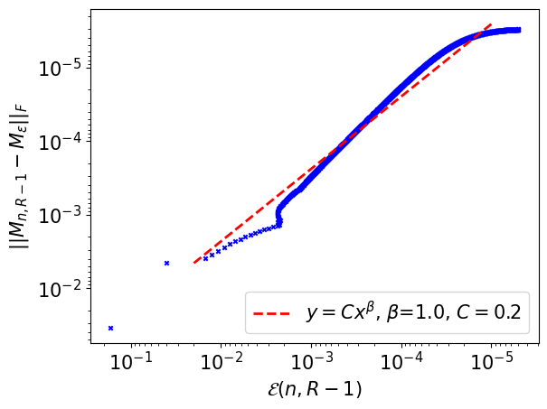
7.1 Convergence of the multi-constrained Sinkhorn algorithm

Refer to caption
Figure 1: Sampled and stressed IVS of the SPX as of 02-09-2024 used to illustrate convergence results.
Refer to caption
Figure 2: Left: convergence of Algorithm 1 performed under the stressed conditions described by Figure 1, as n+n\rightarrow+\infty, with ε=1\varepsilon=1. ||.||F||.||_{F} stands for the Frobenius norm. Right: heatmap of the relative pointwise error between Mn,R1M_{n,R-1} and MεM_{\varepsilon}, after the stopping criterion tol\mathcal{E}_{\mathrm{tol}} was met (n1000n\approx 1000).

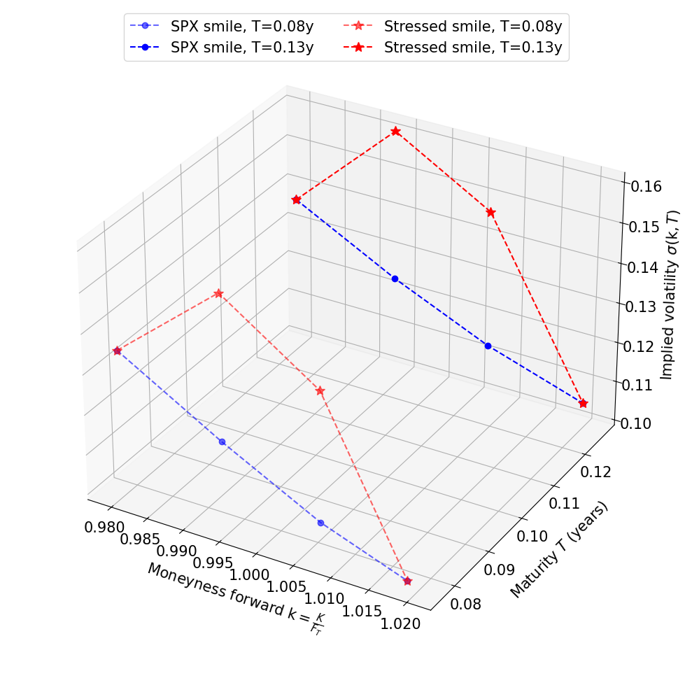
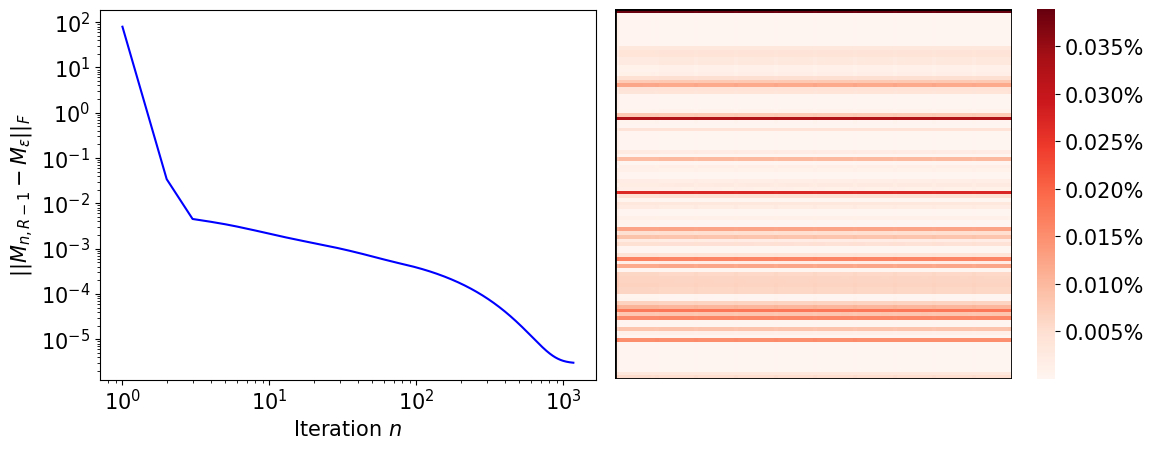
In Figure 1, we artificially created (butterfly) arbitrages by increasing the volatilities around the money by 30%30\%. Numerical illustration of Proposition 6.2.3 can be found in Figure 2. We performed Algorithm 1 starting from the stressed configuration described by Figure 1, with ε=1\varepsilon=1 and tol=5×10⁶\mathcal{E}_{\mathrm{tol}}=5\times 10^{-6}. MεM_{\varepsilon} was obtained using SciPy’s solver minimize with the method SLSQP. In this toy example, R=14R=14. In Figure 2, on the left, we see that the distance between Mn,R1M_{n,R-1} and MεM_{\varepsilon} is monotonically decreasing to zero. However, it is not clear that the rate of convergence is linear, as for the usual Sinkhorn algorithm. On the right, we see that if we zoom in residual errors between Mn,R1M_{n,R-1} (n1000n\approx 1000) and MεM_{\varepsilon}, both matrices are very close, confirming empirically that the algorithm estimates what is expected.

Refer to caption
Figure 3: Empirical relation between (n,R1)\mathcal{E}(n,R-1) and Mn,R1MεF||M_{n,R-1}-M_{\varepsilon}||_{F}, along iterations of Algorithm 1, in the toy example described by Figure 1. The red line was obtained by linear regression in the log space.

Figure 3 gives an idea of the relation between the stopping criterion (n,R1)\mathcal{E}(n,R-1) and the distance to the optimum Mn,R1MεF||M_{n,R-1}-M_{\varepsilon}||_{F}, in the toy example of Figure 1. As a rule of thumb, we can retain that empirically, Mn,R1MεF=𝒪((n,R1))||M_{n,R-1}-M_{\varepsilon}||_{F}=\mathcal{O}\left(\mathcal{E}(n,R-1)\right).

7.2 Convergence of the entropic regularization (ε0\varepsilon\rightarrow 0)

Refer to caption
Figure 4: Evolution of the cost of MεM_{\varepsilon} when ε\varepsilon approaches zero, in comparison with the optimal value of 4.3.2 solved in the situation described by Figure 1.

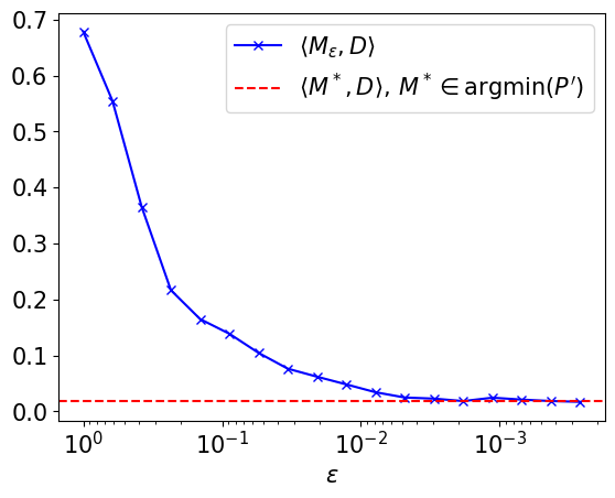
Figure 4 illustrates Proposition 5.1.2: when ε0\varepsilon\rightarrow 0, MεM_{\varepsilon} converges to a minimizer of 4.3.2. We point out that, to obtain this graph, we used the Python library POT [23] to handle classical numerical errors appearing when solving EOT problems for small regularization parameters. Such difficulties are, for example, discussed in [12] Section 4.3.

7.3 Correction of stressed smiles: single maturity case

Refer to caption
Figure 5: Left column: comparison of our method (in green) vs. [13] (in purple), for different types of stress-test (in red), applied to observed SPX smile (in blue). Right column: illustration of the effect of regularization, for the same stress-tests.

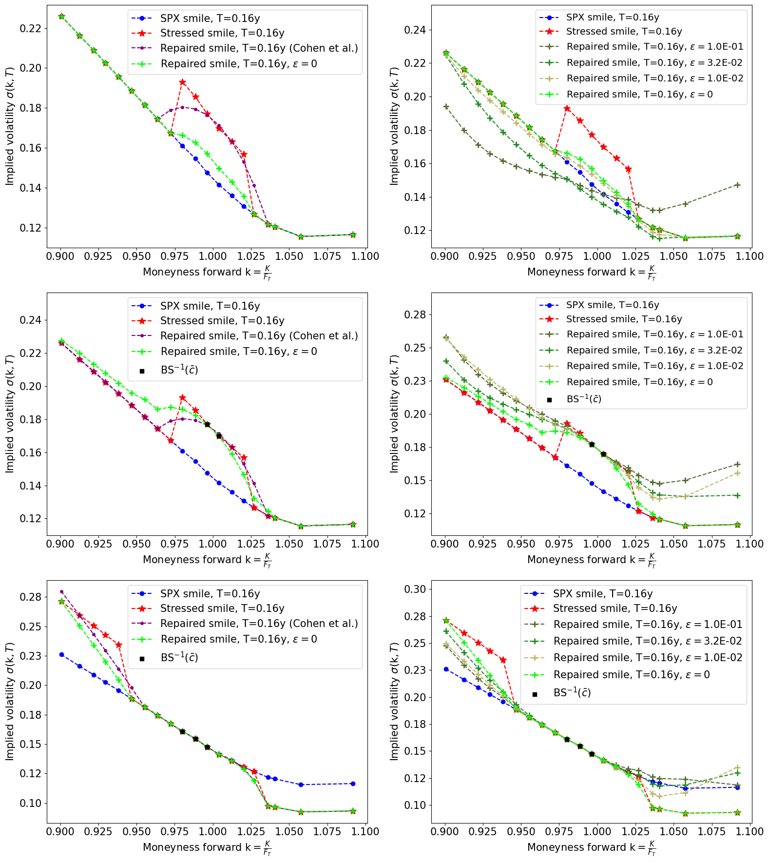
In this section, the SPX data we work with is dated 23-10-2024. Figure 5 highlights the differences between our method and the one proposed in [13], for three types of stress-test. In the first row, the volatilities with moneyness k[0.975,1.025]k\in[0.975,1.025] were increased by 20%20\%. Surprisingly, the green smile with ε=0\varepsilon=0, corresponding to a solution of 4.3, does not deviate from the original blue smile outside the interval [0.975,1.025][0.975,1.025], even though no calibration constraints were imposed. The increase is also more contained than Cohen et al.’s solution. The graph on the right displays the expected behavior of regularization: when ε\varepsilon approaches zero, the darker green smiles are getting closer to the one associated to ε=0\varepsilon=0. We also observe that higher ε\varepsilon tends to produce smoother and more U-shaped smiles. However, without constraints here, the average level of volatility is lost for high regularization.

Regarding the second row, the volatilities with k[0.975,1.025]k\in[0.975,1.025] were still increased by 20%20\%, but we also constrained our solutions to calibrate two prices that were impacted by the stress-test, to ensure high enough volatility at-the-money (see the black squares on the graphs). The green smile with ε=0\varepsilon=0 corresponds then to a solution of 4.3. Again, we observe smoother smiles for greater ε\varepsilon and constraining seems to be an appropriate way to match a certain average level of volatility.

The last row was obtained with a more exotic stress-test of steepening: volatilities with k0.94k\leq 0.94 were raised by 20%20\%, while the ones with k1.03k\geq 1.03 were reduced by 20%20\%. This time, our solutions were constrained to fit some prices that were not affected by the stress-test, to keep the level of volatility around the money unaffected.

Note that all smiles appearing in Figure 5 are arbitrage-free (except of course the stressed ones) and were obtained with tol=104\mathcal{E}_{\mathrm{tol}}=10^{-4}.

Refer to caption
Figure 6: First row: comparison of the marginal obtained with our method vs. the one implied by Cohen et al’s approach, for the first stress-test described in Figure 5. ν+\nu^{+} (in red) and ν\nu^{-} (in orange) are the positive and negative parts of ν\nu as defined in Section 2.2. Second row: illustration of the effect of regularization on the marginals.

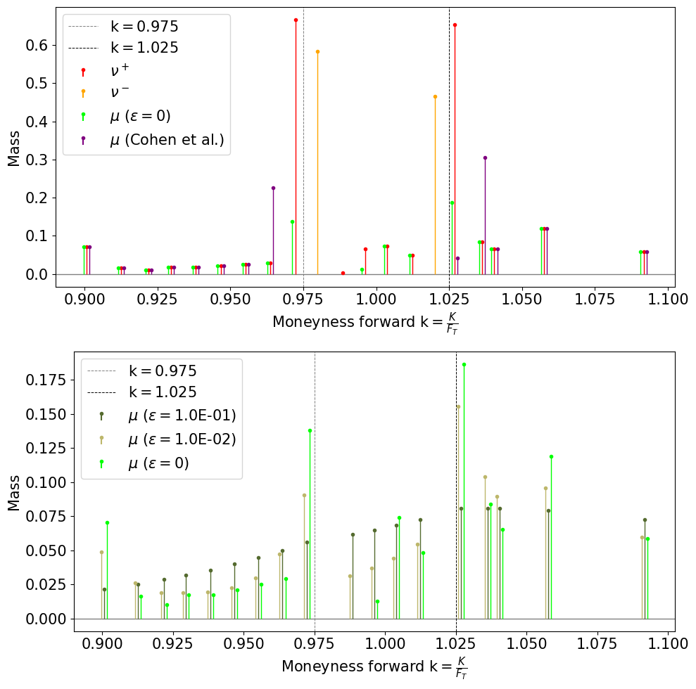
Figure 6 zooms in the distributions of mass (on Θ\{0,kmax}\Theta\backslash\{0,k_{\mathrm{max}}\}, for the sake of graphs’ clarity) of the different marginals attained either by our method or Cohen et al’s, for the first stress-test of Figure 5. Note that, for visualization purposes, the sticks were slightly separated, but they correspond to the same atoms. Regarding the first row, we observe very unusual distributions, from a financial point of view, but still true probability measures. We believe there are two reasons for that. The first is the closeness with respect to the stressed configuration, which is economically not viable, because of arbitrages. The second is the general sparsity of solutions of linear programs (our case) and L1\mathrm{L}^{1}-norm minimization problems (Cohen et al’s case). About the second row, we recognize a typical property of solutions of EOT problems. They are more diffuse than the non-regularized solution and get sparser when ε\varepsilon approaches zero.

7.4 Correction of stressed smiles: two maturities case

In this section, we still use SPX data dated 23-10-2024, with two maturities to highlight the behavior of the projection method in a multidimensional framework.

Refer to caption
Figure 7: Left column: comparison of our method (in green) vs. [13] (in purple), for different types of stress-test (in red), applied to observed SPX smiles (in blue). Right column: illustration of the effect of regularization, for the same stress-tests.

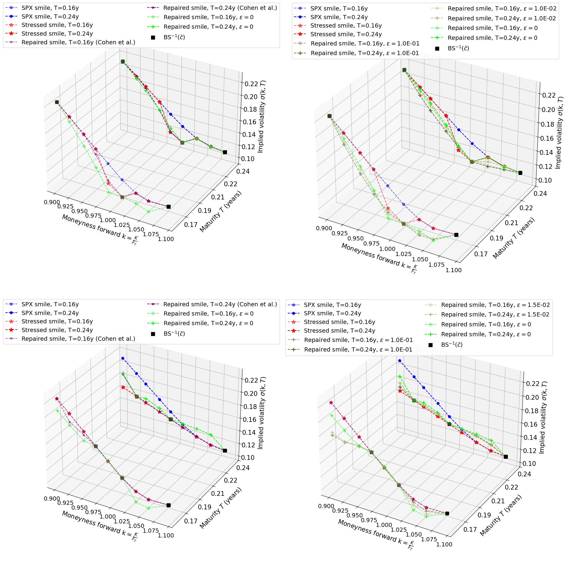
Figure 7 is nothing else but the extension of experiments described in Figure 5 to a two maturities setting. In the first row, the volatilities with moneyness k[0.975,1.025]k\in[0.975,1.025] were decreased by 20%20\%, for both maturities. To have sufficiently low volatility around the money, and to ensure that in and out-the-money volatilities remain, as much as possible, unaffected, we constrained our solution to calibrate a subset of arbitrage-free prices (see the black squares on the graph). In this experiment, the green and purple smiles at T=0.24yT=0.24y are very close, but our correction at T=0.16yT=0.16y deviates more from the red smile than Cohen et al’s. Regularization has again the property to smooth the correction. What is interesting about the second row is that we created calendar arbitrages only, by flattening the smile at the highest maturity. As a consequence, each smile is arbitrage-free when ignoring the other. For this second experiment, we wanted our solutions to preserve the average shape of the smile at T=0.16yT=0.16y and to be as flat as possible at T=0.24yT=0.24y. This is what motivated our choice of calibration subset (see the black squares). Both green and purple corrections are close. However, we observe again that Cohen et al’s output is closer than ours from the stressed surface. Note that we could not achieve a convergence criterion of 10410^{-4} for ε=102\varepsilon=10^{-2}, in this second stress-test, due to numerical instabilities (overflow in exponentials) encountered in the root-finding procedures of certain substeps of Algorithm 1. This is why we only performed regularization up to ε=1.5×10²\varepsilon=1.5\times 10^{-2}. We believe handling these instabilities (addressed, for instance, in [12] Section 4.3) is out of the scope of this work.

As before, all the smiles appearing in Figure 7 are arbitrage-free (except the stressed ones) and were obtained with tol=104\mathcal{E}_{\mathrm{tol}}=10^{-4}.

8 Conclusion

We have explored a novel approach to correct arbitrages in option portfolios, based on the projection of a signed measure onto the subset of martingales, with respect to a Wasserstein distance. We conducted an in-depth study of the associated entropic optimal transport problem and introduced an appropriate Sinkhorn algorithm, for which we proved convergence. We have validated this theoretical framework through numerical experiments, comparing the behavior of our method with existing ones. In future work, we aim at building on this approach to develop a method with an improved computational complexity.

References

  • [1] A. Alfonsi, J. Corbetta, and B. Jourdain. Sampling of probability measures in the convex order by Wasserstein projection. Annales de l’I.H.P. Probabilités et Statistiques, 56(3):1706–1729, 2020.
  • [2] L. Ambrosio, E. Mainini, and S. Serfaty. Gradient flow of the Chapman–Rubinstein–Schatzman model for signed vortices. Annales de l’I.H.P. Analyse non linéaire, 28(2):217–246, 2011.
  • [3] Basel Committee on Banking Supervision. Minimum capital requirements for market risk, 2019. https://www.bis.org/bcbs/publ/d457.pdf.
  • [4] H. H. Bauschke and A. S. Lewis. Dykstras algorithm with Bregman projections: A convergence proof. Optimization, 48(4):409–427, 2000.
  • [5] M. Beiglböck, P. Henry-Labordere, and F. Penkner. Model-independent bounds for option prices—a mass transport approach. Finance and Stochastics, 17:477–501, 2013.
  • [6] J.-D. Benamou, G. Carlier, M. Cuturi, L. Nenna, and G. Peyré. Iterative Bregman projections for regularized transportation problems. SIAM Journal on Scientific Computing, 37(2):A1111–A1138, 2015.
  • [7] J.-D. Benamou, G. Chazareix, and G. Loeper. From entropic transport to martingale transport, and applications to model calibration. arXiv preprint arXiv:2406.11537, 2024. https://arxiv.org/pdf/2406.11537.
  • [8] L. M. Bregman. The relaxation method of finding the common point of convex sets and its application to the solution of problems in convex programming. USSR computational mathematics and mathematical physics, 7(3):200–217, 1967.
  • [9] H. Brezis. Analyse fonctionnelle. Théorie et applications, 1983.
  • [10] P. Carr and D. B. Madan. A note on sufficient conditions for no arbitrage. Finance Research Letters, 2(3):125–130, 2005.
  • [11] Y. Censor and S. Reich. The Dykstra algorithm with Bregman projections. Communications in Applied Analysis, 2(3):407–420, 1998.
  • [12] L. Chizat, G. Peyré, B. Schmitzer, and F.-X. Vialard. Scaling algorithms for unbalanced optimal transport problems. Mathematics of Computation, 87(314):2563–2609, 2018.
  • [13] S. N. Cohen, C. Reisinger, and S. Wang. Detecting and repairing arbitrage in traded option prices. Applied Mathematical Finance, 27(5):345–373, 2020.
  • [14] L. Cousot. Necessary and sufficient conditions for no static arbitrage among European calls. Courant Institute, New York University, 2004.
  • [15] L. Cousot. Conditions on option prices for absence of arbitrage and exact calibration. Journal of Banking & Finance, 31(11):3377–3397, 2007.
  • [16] M. Cuturi. Sinkhorn distances: Lightspeed computation of optimal transport. Advances in neural information processing systems, 26, 2013.
  • [17] M. H. Davis and D. G. Hobson. The range of traded option prices. Mathematical Finance, 17(1):1–14, 2007.
  • [18] H. De March. Entropic approximation for multi-dimensional martingale optimal transport. arXiv preprint arXiv:1812.11104, 2018. https://arxiv.org/pdf/1812.11104.
  • [19] H. De March and P. Henry-Labordere. Building arbitrage-free implied volatility: Sinkhorn’s algorithm and variants. arXiv preprint arXiv:1902.04456, 2019. https://arxiv.org/pdf/1902.04456.
  • [20] R. L. Dykstra. An algorithm for restricted least squares regression. Journal of the American Statistical Association, 78(384):837–842, 1983.
  • [21] European Banking Authority. Draft Regulatory Technical Standards on the capitalisation of non-modellable risk factors under the FRTB, 2020.
  • [22] M. R. Fengler and L.-Y. Hin. Semi-nonparametric estimation of the call-option price surface under strike and time-to-expiry no-arbitrage constraints. Journal of Econometrics, 184(2):242–261, 2015.
  • [23] R. Flamary, N. Courty, A. Gramfort, M. Z. Alaya, A. Boisbunon, S. Chambon, L. Chapel, A. Corenflos, K. Fatras, N. Fournier, L. Gautheron, N. T. Gayraud, H. Janati, A. Rakotomamonjy, I. Redko, A. Rolet, A. Schutz, V. Seguy, D. J. Sutherland, R. Tavenard, A. Tong, and T. Vayer. POT: Python Optimal Transport. Journal of Machine Learning Research, 22(78):1–8, 2021.
  • [24] J. Guyon. Dispersion-constrained martingale Schrödinger problems and the exact joint S&P 500/VIX smile calibration puzzle. Finance and Stochastics, 28(1):27–79, 2024.
  • [25] R. Jarrow and D. B. Madan. Hedging contingent claims on semimartingales. Finance and Stochastics, 3:111–134, 1999.
  • [26] H. W. Kuhn and A. W. Tucker. Nonlinear programming. In Proceedings of the Second Berkeley Symposium on Mathematical Statistics and Probability, pages 481–492, Berkeley, CA, USA, 1951. University of California Press.
  • [27] G. Peyré, M. Cuturi, et al. Computational optimal transport: With applications to data science. Foundations and Trends® in Machine Learning, 11(5-6):355–607, 2019.
  • [28] B. Piccoli, F. Rossi, and M. Tournus. A Wasserstein norm for signed measures, with application to nonlocal transport equation with source term. Communications in Mathematical Sciences, 21(5):1279–1301, 2023.
  • [29] R. Rockafellar. Duality and stability in extremum problems involving convex functions. Pacific Journal of Mathematics, 21(1):167–187, 1967.
  • [30] R. Rockafellar. Convex Analysis. Princeton Landmarks in Mathematics and Physics. Princeton University Press, 1997.
  • [31] R. Sinkhorn and P. Knopp. Concerning nonnegative matrices and doubly stochastic matrices. Pacific Journal of Mathematics, 21(2):343–348, 1967.
  • [32] V. Strassen. The existence of probability measures with given marginals. The Annals of Mathematical Statistics, 36(2):423–439, 1965.
  • [33] C. Villani. Topics in optimal transportation, volume 58. American Mathematical Soc., 2021.
  • [34] C. Villani et al. Optimal transport: old and new, volume 338. Springer, 2009.
  • [35] V. Zetocha. Volatility Transformers: an optimal transport-inspired approach to arbitrage-free shaping of implied volatility surfaces. Available at SSRN, 2023. https://papers.ssrn.com/sol3/papers.cfm?abstract_id=4623940.

Appendix A Reminders on convex analysis

We fix dd\in\mathbb{N}^{*} and denote by .,.\langle.,.\rangle the usual scalar product in d\mathbb{R}^{d}.

Definition A.1 (Affine hull and relative interior).

Let AA be a subset of d\mathbb{R}^{d}. The affine hull of AA, aff(A)\mathrm{aff}(A), is the smallest affine set of d\mathbb{R}^{d} containing AA. The relative interior of AA, ri(A)\mathrm{ri}(A), is the interior of AA, when AA is seen as a subset of its affine hull endowed with the subspace topology:

ri(A)={xA|ε>0,Bε(x)aff(A)A},\mathrm{ri}(A)=\left\{x\in A\,|\,\exists\varepsilon>0,\,B_{\varepsilon}(x)\cap\mathrm{aff}(A)\subset A\right\}\,,

where Bε(x)B_{\varepsilon}(x) is the open ball centered at xx, with radius ε\varepsilon.

Definition A.2 (Indicator function of a set).

Let AA be a subset of d\mathbb{R}^{d}. The indicator function of AA is defined by

ιA(x)={0 if xA+ if xA.\iota_{A}(x)=\left\{\begin{array}[]{l}0\text{ if }x\in A\\ +\infty\text{ if }x\notin A\end{array}\right.\,.

Recall that if AA is non-empty, closed and convex in d\mathbb{R}^{d}, then ιA\iota_{A} is convex, lower semicontinuous and ιA+\iota_{A}\not\equiv+\infty (i.e. ιA\iota_{A} is proper).

Definition A.3 (Domain of a function).

Let f:d],+]f:\mathbb{R}^{d}\rightarrow\,]-\infty,+\infty]. The domain of ff, denoted by dom(f)\mathrm{dom}(f), is the set

{xd|f(x)<+}.\{x\in\mathbb{R}^{d}\,|\,f(x)<+\infty\}\,.
Definition A.4 (Convex conjugate).

Let f:d],+]f:\mathbb{R}^{d}\rightarrow]-\infty,+\infty]. The convex conjugate of ff is defined for each ydy\in\mathbb{R}^{d} by

f(y)=supxdx,yf(x).f^{*}(y)=\underset{x\in\mathbb{R}^{d}}{\sup}\;\langle x,y\rangle-f(x)\,.
Definition A.5 (Subdifferential).

Let f:d],+]f:\mathbb{R}^{d}\rightarrow]-\infty,+\infty]. The subdifferential of ff at the point xdx\in\mathbb{R}^{d} is the set

f(x)={yd|f(z)f(x)y,zx, for all zd}.\partial f(x)=\left\{y\in\mathbb{R}^{d}\,|\,f(z)-f(x)\geq\langle y,z-x\rangle\,,\text{ for all }z\in\mathbb{R}^{d}\right\}\,.

Note that it might be empty (for instance when xdom(f)x\notin\mathrm{dom}(f)). Whenever it is not, ff is said to be subdifferentiable at xx. An element of f(x)\partial f(x) is called a subgradient of ff at xx. If ff is differentiable at xx, one can prove that f(x)={f(x)}\partial f(x)=\left\{\nabla f(x)\right\}. Besides, xargminydf(y)x\in\underset{y\in\mathbb{R}^{d}}{\mathrm{argmin}}\;f(y) if and only if ff is subdifferentiable at xx and 0f(x)0\in\partial f(x).

Theorem A.6 (Theorem 23.8 in [30]).

Let nn\in\mathbb{N}^{*}, f1,,fnf_{1},\cdots,f_{n} be proper convex functions on d\mathbb{R}^{d} and let f=i=1nfi\displaystyle f=\sum_{i=1}^{n}f_{i}. Then,

f1(x)++fn(x)f(x),xd,\partial f_{1}(x)+\cdots+\partial f_{n}(x)\subset\partial f(x),\,\forall x\in\mathbb{R}^{d}\,,

where the sum is to be understood in the Minkowski sense.

Furthermore, if i=1nri(dom(fi))\displaystyle\bigcap_{i=1}^{n}\mathrm{ri}(\mathrm{dom}(f_{i}))\neq\emptyset, then the equality holds for all xdx\in\mathbb{R}^{d}.

The following results are stated in a finite dimensional framework, which is sufficient for us, but they were also proved in more general settings.

Proposition A.7 (Proposition 1.9 in [9]).

Let f:d],+]f:\mathbb{R}^{d}\rightarrow]-\infty,+\infty]. If ff is proper (i.e. f+f\not\equiv+\infty) lower semicontinuous and convex, then ff^{*} is also proper, lower semicontinuous and convex.

Theorem A.8 (Fenchel-Moreau, see Theorem 1.10 in [9]).

Let f:d],+]f:\mathbb{R}^{d}\rightarrow]-\infty,+\infty] be a proper, lower semicontinuous and convex function. Then, f=ff^{**}=f.

Theorem A.9 (Fenchel-Rockafellar, [29]).

Let T:dmT:\mathbb{R}^{d}\rightarrow\mathbb{R}^{m} be a linear map and T:mdT^{\dagger}:\mathbb{R}^{m}\rightarrow\mathbb{R}^{d} its adjoint. Let f:d],+]f:\mathbb{R}^{d}\rightarrow]-\infty,+\infty] and g:m],+]g:\mathbb{R}^{m}\rightarrow]-\infty,+\infty] be proper, lower semicontinuous and convex functions. If there exists xdom(f)x\in\mathrm{dom}(f) such that gg is continuous at TxTx, then

supxdf(x)g(Tx)=minymf(Ty)+g(y),\underset{x\in\mathbb{R}^{d}}{\sup}\;-f(-x)-g(Tx)=\underset{y\in\mathbb{R}^{m}}{\min}\;f^{*}(T^{\dagger}y)+g^{*}(y)\,,

i.e. the right-hand side is attained.

Moreover, xx is a maximizer of the left-hand side if and only if there exists a minimizer yy of the right-hand side, such that xf(Ty)-x\in\partial f^{*}(T^{\dagger}y) and yg(Tx)y\in\partial g(Tx).