An optimized absorbing potential for ultrafast, strong-field problems
Abstract
Theoretical treatments of strong-field physics have long relied on the numerical solution of the time-dependent Schrödinger equation. The most effective such treatments utilize a discrete spatial representation — a grid. Since most strong-field observables relate to the continuum portion of the wave function, the boundaries of the grid — which act as hard walls and thus cause reflection — can substantially impact the observables. Special care thus needs to be taken. While there exist a number of attempts to solve this problem — e.g., complex absorbing potentials and masking functions, exterior complex scaling, and coordinate scaling — none of them are completely satisfactory. The first of these is arguably the most popular, but it consumes a substantial fraction of the computing resources in any given calculation. Worse, this fraction grows with the dimensionality of the problem. And, no systematic way to design such a potential has been used in the strong-field community. In this work, we address these issues and find a much better solution. By comparing with previous widely used absorbing potentials, we find a factor of 3–4 reduction in the absorption range, given the same level of absorption over a specified energy interval.
I Introduction
To theoretically describe highly nonperturbative interactions — such as strong-field physics — in a fully quantitative manner, the best option is usually to numerically solve the time-dependent Schrödinger equation (TDSE). One of the most popular approaches to practically solving the TDSE represents the wave function on a finite spatial grid with boundary conditions applied at its edges. In general, such a grid needs to be large enough so that there are no reflections from the boundaries which behave as infinitely hard walls. Otherwise, the reflections might lead to unphysical changes in the observables. For example, an ionized wavepacket reflected from the boundary back to the origin might be driven by the laser field into bound states, thus reducing the total ionization yield.
The most direct way to avoid such spurious reflections is to move the boundary further away. Since the grid density is fixed physically by the highest energy, however, this requires more grid points which, in turn, incurs a greater computational cost. In fact, the large grids required to describe current experiments have become a key bottleneck to improving the numerical efficiency of solving the TDSE, especially as laser wavelengths push beyond 800 nm.
Fortunately, if the wave function at large distances can easily be reconstructed or is not of interest, it can be absorbed at a sufficiently large distance that it does not affect the dynamics at small distances. Applying such absorption techniques, one can generally reduce the box size significantly. The absorb-and-reconstruct strategy was probably first developed by Heather and Metiu Heather and Metiu (1987) which they demonstrated for strong-field dissociation. Their work has been adopted in hundreds of papers since. A new implementation following this philosophy Tao and Scrinzi (2012); Morales et al. (2016) has proven similarly effective.
Among the various methods to effect absorption at the boundary, the most widely used — and probably the simplest — method is the complex absorbing potential (CAP) Kosloff and Kosloff (1986); Vibok and Balint-Kurti (1992a, b); Macias et al. (1994); Riss and Meyer (1996); Ge and Zhang (1998); Hussain and Roberts (2000); Manolopoulos (2002); Poirier and Carrington (2003); Muga et al. (2004); Tarana and Greene (2012); Strelkov et al. (2012); Yue and Madsen (2013); Krause et al. (2014) or the closely related masking function Krause et al. (1992). Another increasingly popular absorbing-boundary technique is exterior complex scaling Rescigno et al. (1999); Rescigno and McCurdy (2000); He et al. (2007); Tao et al. (2009); Scrinzi (2010), where one rotates the coordinate into the complex plane at large distances. Other, less common, methods to treat the boundary reflection include time-dependent coordinate scaling Sidky and Esry (2000); Hamido et al. (2011); Miyagi and Madsen (2016), the interaction representation Zhang (1990); Williams et al. (1991); Yao and Chu (1992), and Siegert-state expansions Yoshida et al. (1999). While these methods are local in time and vary from exact to approximate, it is also possible to construct a perfectly transparent boundary using Feshbach projection techniques Muga et al. (2004). The disadvantage of such methods is that they require the wave function from previous times and are thus nonlocal in time. In this work, we will focus on the CAP due to its popularity and the simplicity of its implementation. Our goals are to make it both more efficient and more effective.
Although the CAPs utilized in previous studies are predominantly polynomials Riss and Meyer (1996); Ge and Zhang (1998); Poirier and Carrington (2003); Muga et al. (2004); Tarana and Greene (2012); Yue and Madsen (2013); Krause et al. (2014), other types of absorbing potentials such as Strelkov et al. (2012), Pöschl-Teller () Kosloff and Kosloff (1986), and a pseudo-exponential [] Vibok and Balint-Kurti (1992a, b) have also been used. In most of these papers, the CAP’s performance is examined by studying the dependence of the reflection and transmission coefficients on the energy. Riss and Meyer Riss and Meyer (1996), for instance, carefully investigated the properties of and for polynomial CAPs, finding some difficulty in treating low energies. They characterized their optimized potential parameters in terms of the absorbed energy ratio , where and indicate the minimum and maximum energies, respectively, for which absorption exceeds a given value. The maximum ratio they considered, 30, is too small, however, for typical strong-field electronic dynamics. We will, for instance, consider =500. Vibok and Balint-Kurti Vibok and Balint-Kurti (1992a, b) presented a more optimal CAP — the type — for heavy particles, but the range of absorbed energies was still insufficient for strong-field problems.
Even though and provide a clear, quantitative measure of performance, studies of CAPs in strong-field problems utilizing them can hardly be found. Their absence is likely due to the inherent time-dependent nature of the strong-field problem and the authors’ consequent focus on wavepacket behavior, losing track of the connection with and . In contrast, we will adopt as the figure of merit for designing our absorbing potentials for the strong-field problem, incorporating it as a critical piece in our systematic CAP construction method.
The major advantage of the CAP is its simplicity. The major disadvantage is that it has required a relatively large spatial range to be effective, thus consuming non-negligible computational resources. In this paper, we improve the performance of the CAP and systematically design a more optimal — yet general — CAP for strong-field processes. Specifically, we provide an optimized CAP with a factor of 3–4 reduction in the absorption range compared to some widely-used CAPs Muga et al. (2004). Our optimized CAP absorbs at a prescribed level over a large enough energy range to be useful for strong-field processes.
To be clear, while we optimize our CAP for the strong-field problem, it can be readily adapted and re-optimized for other problems following the procedures we outline below.
II Theoretical background
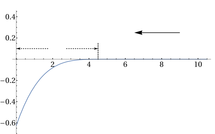
Since a time-dependent wavepacket can always be written as a superposition of the time-independent scattering states, we use the time-independent reflection coefficient as a quantitative tool for characterizing and designing an optimal CAP. We will require the CAP’s reflection coefficient to remain below a cutoff value , , over a given energy range . Since the spatial region devoted to the CAP near the edge of the grid is unphysical, we wish to minimize the computing resources it consumes as much as possible. Therefore, in this work, our optimization efforts focus on reducing the absorption range , as defined in Fig. 1, while meeting the absorption criteria above.
| CAP type | (units of ) |
|---|---|
| quadratic Riss and Meyer (1996); Muga et al. (2004) | |
| cosine masking function Krause et al. (1992) | |
| M-JWKB Manolopoulos (2002) | |
| quartic Riss and Meyer (1996); Muga et al. (2004) | |
| pseudo-exponential Vibok and Balint-Kurti (1992a) | |
| Pöschl-Teller Kosloff and Kosloff (1986) | |
| single-exponential (present) | |
| double-exponential (present) | |
| double-sinh (present) | |
We study one-dimensional CAPs since they can be easily adapted to higher dimensions, obtaining the reflection coefficient by solving the Schrödinger equation,
| (1) |
as indicated schematically in Fig. 1. We consider the potential to be one of the CAPs listed in Table 1. The shapes of all the CAPs considered are generically as in Fig. 1 and are controlled by the following parameters: is the strength of the potential, mainly determines its width, and is a shift. These are the parameters that will be varied to optimize the CAPs.
The JWKB-based CAP obtained by Manolopoulos Manolopoulos (2002) — labeled M-JWKB in Table 1 — is qualitatively different from the others, however, in that it requires no optimization. This simplicity is certainly one of its strengths and derives from the fact that its reflection coefficient effectively decreases monotonically from unity at zero energy to at infinite energy. Its explicit expression is in terms of the Jacobi elliptic function ,
| (2) |
with = where = Manolopoulos (2002). One simply chooses from the condition .
The first five CAPs in the table are defined to be non-zero only for and to vanish identically for . The remaining CAPs are defined for all , but vanish exponentially with . The first four CAPs are some of the most commonly used, with the cosine masking function recast as a CAP using .
We include the Pöschl-Teller potential because it is well known to be reflectionless for specific real values of , suggesting that it might have advantageous properties as a CAP. It can be shown analytically, however, that this property no longer holds for complex . In the process of optimizing it for the present purposes, we found that shifting its center off the grid minimized , leaving only its exponential tail on the grid. This result suggested using instead the simpler family of exponential CAPs included in the table.
We calculate the reflection coefficient numerically using the finite-element discrete-variable representation (FEDVR) McCurdy et al. (2001); Schneider et al. (2006) and eigenchannel R-matrix method Aymar et al. (1996). The reflection coefficient can also be calculated analytically for several of the potentials in Table 1. However, we give the analytic solutions (derivations in the appendices) only for the CAPs we propose — namely, the single-exponential and double-exponential CAPs. The double-sinh potential has no analytic solution to the best of our knowledge. In these cases, we confirmed that the R-matrix reflection coefficients agreed with the analytical to several significant digits.
Since our primary goal is to systematically design an absorbing potential for the strong-field ionization problem with predetermined properties, we will use atomic units for the remainder of our discussion. Our results can be readily applied to other problems, though, using the derivations in the appendices in which the masses and SI units are explicitly retained.
III Optimization of Proposed CAPs
We demonstrate our optimization procedure in detail below first for the single-exponential CAP since it is the simplest to optimize. It also establishes a few key results important for the optimization of our recommended CAPs: the double-exponential and double-sinh potentials. Whether the solution is analytical or numerical, the procedure we describe for optimization is the same and can be applied to other CAPs as well. In fact, this is what we have done for the comparison in Sec. IV.
The values of , , and that we will focus on for this discussion are
| (3) |
We chose this energy range to cover for an 800-nm laser pulse at ( is the pondermotive energy: with the intensity and the laser frequency). This energy range includes essentially all photoelectrons one would expect to be produced in this typical pulse. In momentum, which is more convenient for the analytical , this range corresponds to
| (4) |
Note that 14 exceeds the highest-energy electrons one would normally expect in a strong-field problem, but we will show below that this choice has little effect on the resulting . Finally, we use = to define from =.
III.1 Single-Exponential CAP
We take the single-exponential CAP to have the form
| (5) |
Its reflection coefficient, as shown in App. A, is
| (6) |
where the unitless momentum is with and the unitless potential strength is . To achieve our goal of minimizing , we must find the optimal and .
III.1.1 Purely imaginary potential
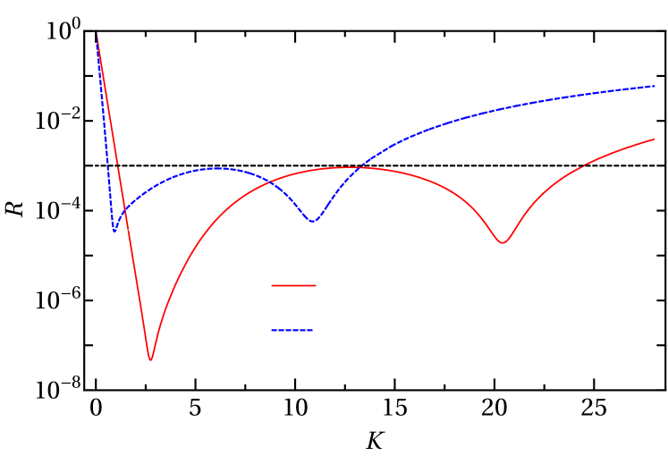
For a purely imaginary potential, , Fig. 2 shows the behavior of as a function of . As the figure suggests, one can show from Eq. (6) that
| (7) |
As can also be seen in the figure, increasing the strength of the CAP means this exponential decrease continues to larger and the large- tail decreases.
We can thus use Eq. (7) to write
| (8) |
giving
for . From , the scale is therefore determined:
We can now find the required from
| (9) |
since =. Solving this equation gives
| (10) |
This example illustrates the fact that can only be substantially decreased if is decreased. Thus, and determine , and is set by the form of the CAP and its parameters. In general, the smaller is, the more difficult absorption becomes. Roughly speaking, this behavior can be traced to the need for to be large enough for the potential to contain the longest wavelength to be absorbed.
III.1.2 Complex potential
Given , decreasing further requires decreasing . This is not possible with a purely imaginary single-exponential CAP, so we must allow to be complex.
The reflection coefficient in Eq. (6) still holds for complex and looks generically like those displayed in Fig. 2 — with the exception that
| (11) |
This small- behavior suggests that the best way to reduce — and thus and — is to make small (since must be positive to have absorption). That is, we should make much larger than . The fastest decay one can achieve with this approach is which, in turn, sets the limit on how small can be.
The physical origin of this faster low- decrease is clear: the real part of the potential is attractive and accelerates the wave before it encounters the imaginary part of the potential Muga et al. (2004). Absorption thus occurs at a shorter wavelength where absorption can be efficient with a much smaller . Since must be large enough for sufficient absorption, however, cannot be zero. The optimum value will be a compromise between these two factors.
To determine the magnitude of the improvement in , we use and the small- behavior in Eq. (11) to write
| (12) |
From this, we can find and for a given . Combining everything and simplifying reduces the problem to solving Eq. (9) for with from Eq. (6). The resulting as a function of is shown in Fig. 3.
The figure shows that the optimization problem has been reduced to a one-dimensional minimization of with respect to . As expected, the solution,
| (13) |
at =0.055 (with ), lies at small . Adding a real part to the absorbing potential has thus reduced the absorption range by 32% over the purely imaginary single-exponential CAP.
Figure 3 also shows that at the optimal , the potential is 2.62 a.u. deep. This is roughly equal to , leading to local kinetic energies of approximately and thus requiring a much denser spatial grid in the absorption region. Guided by the figure, however, we see that a modest few-percent increase in to 58.9 a.u. () reduces to 1.25 a.u., making it more computationally attractive. Further reduction in can, of course, be achieved — at the expense of .
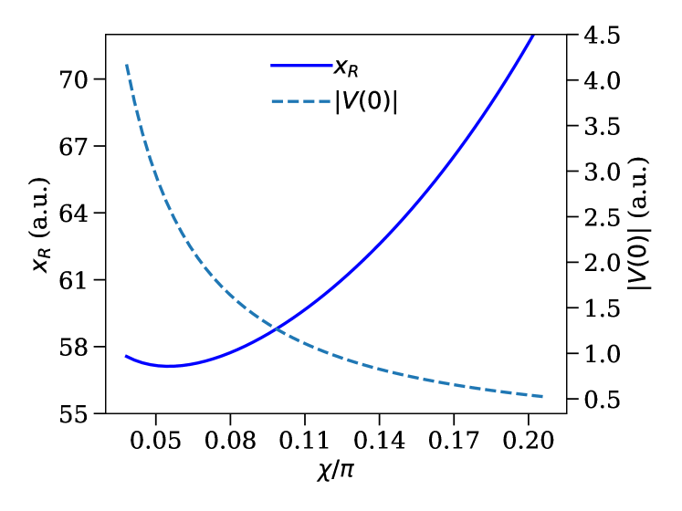
Figure 4 shows the optimum for both the purely imaginary single-exponential CAP of the previous section and the complex single-exponential CAP of the present section. The coefficients satisfy for different ranges of the scaled momentum but the same range of the physical momentum . The range of covered by the complex CAP is smaller than for the imaginary CAP by the ratio of their respective ’s.
III.2 Double-Exponential CAP
It has long been known, of course, that adding a real potential improves CAP performance Muga et al. (2004). And, given the improvement to the single-exponential CAP afforded by doing so, it is natural to ask whether we can do even better with a more flexible complex potential.
Since we want to retain the ability to calculate analytically and since the real part must have longer range than the imaginary part, we choose the CAP to be
| (14) |
The reflection coefficient, as shown in App. B, can be written in terms of the confluent hypergeometric function as
| (15) |
where
III.2.1 and independent
Given the extra potential parameter, optimizing the double-exponential CAP is clearly more challenging than for the single-exponential CAP. And, the complicated expression for only exacerbates the task. It would therefore be convenient to find a regime in which and are independent since this would greatly simplify the optimization.
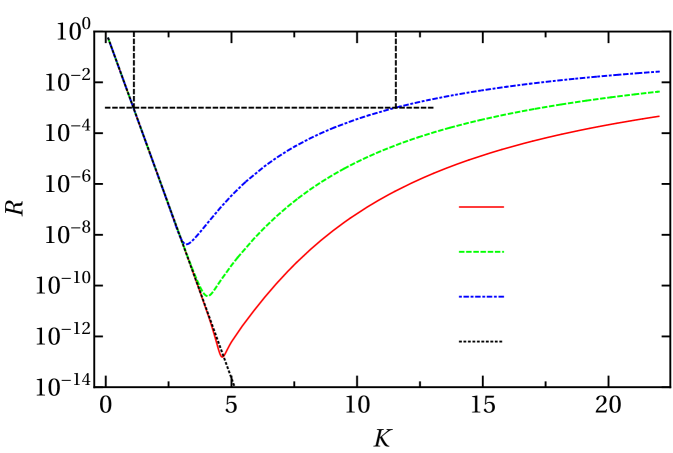
To this end, we show in Fig. 5 the dependence of on and . Generally speaking, — the coefficient of the longer-ranged, real part of — controls the low-energy behavior, while — the coefficient of the shorter-ranged, imaginary part of — controls the high-energy behavior. The underlying physical reasons for these connections are the same as discussed for the single-exponential CAP.
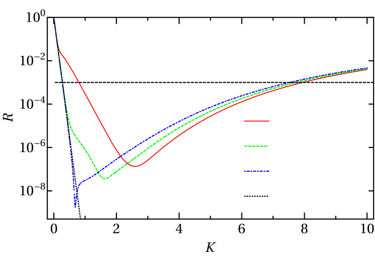
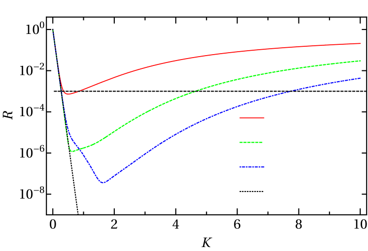
Figure 5 also shows that for and large enough,
| (16) |
for . This behavior immediately shows the benefit of the double exponential since it falls faster than is possible with a single exponential, Eq. (11), leading to a smaller and thus a smaller .
In the regime that Eq. (16) holds, is independent of and and takes the value
| (17) |
For =, = which is indeed much smaller than was possible with the single-exponential CAP.
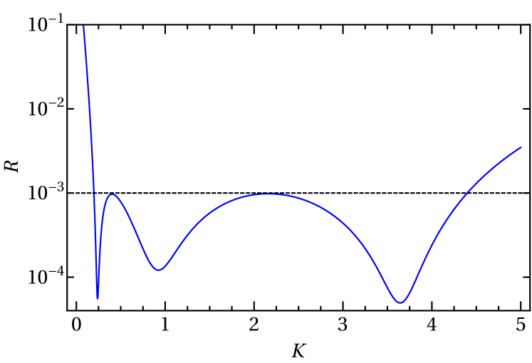
Minimizing now requires fixing to a large enough value that Eq. (16) holds ( is typically sufficient) and solving Eq. (9) for . Using from Eq. (15) and =6.125, we find, for instance,
| (18) |
and the reflection coefficient shown in Fig. 6. There are, however, any number of combinations of and that satisfy Eq. (9). Since for the double-exponential CAP is determined to a very good approximation by alone, though, one would typically choose the smallest possible to obtain the smallest possible . At the same time, it should be noted that , so it is not terribly sensitive to small changes in . Choosing the smallest , however, also ensures that is minimized, thereby keeping the numerical cost down.
III.2.2 and not independent
Although =42.4 a.u. is a significant improvement over the single-exponential result, =57.1 a.u., we can do better. The way to do this is to consider smaller where there are particular combinations of and for which falls off faster than Eq. (16). Such behavior permits smaller and thus smaller . Of course, and are no longer independent in this regime, but it is still true that largely — but not as completely as above — controls and , .
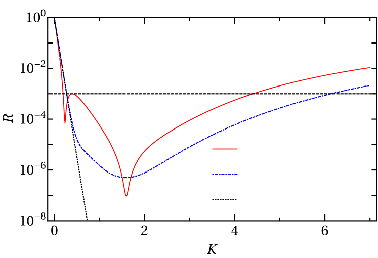
Figure 6 illustrates the small- behavior that we want to take advantage of. For this combination of and , dips below the exponential from Eq. (16) for as seen in the figure. At this and other such parameter combinations, a local minimum develops in at near as shown in the figure. In practice, one searches for these combinations to minimize while simultaneously ensuring that the local maximum in remains below .
To find the minimum value of , we take advantage of its weak dependence on by first minimizing with respect to for some reasonable choice of . With this value of , we then solve Eq. (9) for . Since there is a weak dependence on , though, must be re-minimized for with this new . Then, Eq. (9) must again be solved and the iteration continued until sufficient convergence in and is obtained. Typically, only a handful of iterations are necessary to find 3 digits. More sophisticated methods of performing the constrained minimization of could, of course, be employed as well.
As above, there are many combinations of and that give the smallest , . But, our ultimate goal of minimizing leads us to choose the smallest possible. One convenient example for the optimal values is
which leads to
The corresponding is shown in Fig. 6. Although difficult to prove, this choice appears to be the global optimum for this choice of , , and .
III.3 Double-sinh CAP
While straightforward, the optimization procedure outlined above for achieving such a substantial reduction in is somewhat tedious. Fortunately, it needs to be done only once for a given and ratio . Should one wish to change or only one of the energy limits, however, re-optimization is required. It turns out, though, that the latter limitation can be lifted without compromising on .
In general, one expects the reflection coefficient to be unity for and , and this is the behavior displayed by all the reflection coefficients we have shown. Consequently, the reflection coefficient necessarily satisfies at both low and high energies. As mentioned in Sec. II, however, the M-JWKB CAP Manolopoulos (2002) produces an that decreases more-or-less monotonically to a value controllably less than unity at infinite energy. Its parameters thus do not depend on , removing the need for re-optimizing with changes in either or . Unfortunately, for the M-JWKB CAP turns out to be 118 a.u. because its falls off relatively slowly at low energies, leading to a large .
To retain both the small found for the double-exponential CAP and the advantageous high-energy behavior of the M-JWKB CAP, we have designed the double-sinh CAP:
| (19) |
At large distances, this CAP reduces exactly to the double-exponential CAP, thus possessing its nice long-wavelength, low-energy properties. At short distances, this CAP is dominated by the divergence of the second term. It is this behavior that is inspired by the M-JWKB CAP and that leads to similarly desirable high-energy behavior.
Unlike the single- and double-exponential CAPs, for the double-sinh potential is not analytic as far as we know (unless =0 — in which case, it reduces to one-half of the generalized Pöschl-Teller potential Pöschl and Teller (1933)). We must thus calculate numerically, and the optimal result is shown in Fig. 7 along with the optimal double-exponential result for comparison. Their absorption ranges are =28.8 a.u. and =29.9 a.u., respectively, confirming that there is no compromise on . We note that the qualitative behavior of the double-sinh shown is typical for this CAP.
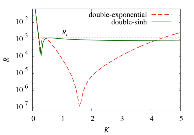
From the figure, the similarity of the two reflection coefficients at low energies is evident. Specifically, the value of — which has the biggest influence on — is nearly identical between the two. In fact, the optimal values of from the double-exponential CAP provide a very good initial guess for the optimization of the double-sinh CAP.
Also evident from Fig. 7 is the difference in the two CAPs’ at high energies. Where the double-exponential rises back towards unity at high energies, the double-sinh asymptotes to a value less than unity. This value can be approximately calculated, by considering only the behavior of , to be
| (20) |
consistent with the limiting behavior found in Ref. Manolopoulos (2002).
Given the discussion in Sec. III.1.2, one might wonder whether allowing the to be complex — rather than real as assumed so far — could improve the CAPs’ performance even further. The simple answer is that it can. In fact, the double-sinh CAP plotted in Fig. 7 has complex . We could not, however, find a more optimal double-exponential CAP by allowing to be complex for the present , , and (see, however, Sec. V.2).
Incidentally, Eq. (20) gives the reflection coefficient at all energies for a CAP that has the form everywhere (see App. D). In particular, the reflection coefficient is not unity at zero energy like the other CAPs we consider and thus corresponds to =0. In many ways, such a CAP would be ideal — no optimization would be necessary and could simply be calculated by setting Eq. (20) to . Unfortunately, =110 a.u. for such a CAP, rendering it uncompetitive with our best CAP — although better than the quadratic CAP often used in the literature (see Table 2).
One possible solution would be to simply cut the CAP off at some . Intuitively, this should affect the low-energy behavior of for wavelengths comparable to and larger than . The reflection coefficient in this case is again analytic (see App. D), and it can be seen after some exploration that while this expectation is true, falls off at small more-or-less like rather than like the exponential decrease of our best CAPs. Since one chooses for this CAP from
| (21) |
— and thus — winds up being large. For instance, =57 a.u. for , which is about double that for our best CAP.
In the context of this discussion, the double-sinh CAP can be seen as providing a smooth cutoff of the CAP and similarly leads to modifications of Eq. (20) at small energies.
Fall-to-the-center problem
Whenever an attractive potential is used, one must take care to consider the “fall-to-the-center” problem. The real-valued version of such potentials are known Landau and Lifshitz (1977) to have an infinite number of bound states with energies stretching to — a fact reflected in the wave function’s oscillating an infinite number of times as — so long as the potential strength exceeds a critical value. This is the quantum-mechanical analog of the classical fall-to-the-center problem in such potentials. Moreover, this effect is possible even for potentials that are only for small like our double-sinh CAP.
No finite numerical representation — such as the grid methods common for TDSE solvers — can represent the infinity of oscillations in the fall-to-the-center regime, and any attempt to accurately represent even a finite number of them will be very costly computationally.
To understand how to avoid this regime, we must examine the small- behavior of the wave function. From App. D and using its notation, we see that
This solution assumes and shows that even for a nearly purely imaginary CAP, =0, the wave function oscillates an infinity of times as . Empirically, choosing so that the first term above suppresses the wave function for is sufficient to prevent numerical difficulties. Consequently, we have chosen =0, which is equivalent to .
III.4 Complex boundary condition
We have so far assumed that the wave function vanishes on the boundary at as is typical for most TDSE solvers. But, if the numerical method used to solve the TDSE is flexible enough to allow complex log-derivative boundary conditions, then additional absorption can be built in at very little additional cost.
The effect of the complex boundary condition,
| (22) |
can be most easily illustrated for a free particle. If one imposes Eq. (22) at =0 as in Fig. 1, but with no potential, one obtains the reflection coefficient (see App. C for more details, including the effect on bound-state energies)
| (23) |
with . To have absorption, we must have ; to have maximum absorption, we must have =0. Thus, setting , we see that at . Such a boundary condition therefore makes the boundary perfectly transparent to an incident plane wave of momentum and partially transparent to other momenta. Moreover, it does so with =0.
Unfortunately, this boundary condition by itself cannot compete with the CAPs since cannot be made small enough over a large enough energy range. Since implementing it, in principle, requires no change in the spatial grid, though, the possibility of combining it with a CAP and reducing further is worth exploring.
At low energies, the CAP will dominate the behavior of , and the boundary condition will have little influence. Therefore, one should try to use the boundary condition to modify the high-energy where it can dominate the behavior. In general, choosing is a good initial guess and allows the reduction of — and therefore .
It should be noted that a complex boundary condition cannot be used with the double-sinh CAP due to its singularity at the boundary. Like the centrifugal potential that it resembles, the double-sinh CAP has one regular solution that vanishes at the boundary and one irregular solution that diverges at the boundary Manolopoulos (2002). Therefore, it is not possible to form the necessary linear combinations to satisfy Eq. (22).
III.4.1 Single-exponential CAP
The reflection coefficient for a single-exponential CAP with a complex boundary condition is again analytic and is given in Eq. (55). The CAP parameters must be re-optimized along with the value of , and the procedure is largely the same as described above. The fact that is essentially unaffected by the addition of the complex boundary condition — so long as — simplifies the process.
Examples of optimal choices are shown in Fig. 8 for a purely imaginary CAP and a complex CAP. Comparison with the reflection coefficients shown in Sec. III.1 shows the effect of the complex boundary condition through the appearance of the high-energy minimum close to . In both cases, the complex boundary condition has produced a roughly 15% reduction in to 71.7 a.u. and 48.1 a.u., respectively.
III.4.2 Double-exponential CAP
Adding a complex boundary condition to the double-exponential CAP also produces an analytic expression for as given in Eq. (56). Re-optimizing the parameters yields the reflection coefficient shown in Fig. 9. As with the single-exponential CAPs, the boundary condition has introduced a high-energy minimum near . Unlike the single-exponential CAPs, though, the minimum was found for .
This optimum double-exponential CAP continues the pattern that has emerged as we have found improved CAPs: namely, that we add more structure to and decrease the absorption for the mid-range of . The double-exponential-CAP reflection coefficients in Fig. 6, for instance, have comparatively little structure — mainly a minimum in . Moreover, this minimum is relatively broad and orders of magnitude lower than . The shown in Fig. 9, in contrast, has three narrower minima only one order of magnitude or so lower than .
IV Optimal CAP
To determine which CAP — among those listed in Table 1 — is the best, we numerically searched for their optimal parameters, assuming they are purely imaginary potentials. From the discussion above, we know that each could be improved by including a real potential and a complex boundary condition, but we expect — and confirmed with spot tests — that the relative performance of the CAPs will remain qualitatively the same. As mentioned previously, we selected the CAPs to compare based on their apparent popularity in the literature or on the claims made for their performance.
In optimizing these CAPs, we follow the principles described in previous sections that the width of the CAP determines the long-wavelength absorption; and the depth, the short-wavelength. The optimization is then reasonably straightforward once we identify the parameters corresponding to the width and depth.
| CAP type | or (, ) | ||||
| quadratic | — | 129 | 124 | ||
| cosine masking function | 15.9 | 810 | 128 | 124 | |
| M-JWKB | — | — | 119 | 118 | |
| quartic | — | 112 | 95 | ||
| pseudo-exponential | 240 | 88 | |||
| Pöschl-Teller | 11.0 | 20.3 | 40.0 | 85 | |
| single-exponential | 10.0 | — | 84 | ||
| single-exponential+BC | 10.0 | — | 72 | ||
| single-exponential | 5.62 | — | 57 | ||
| single-exponential+BC | 5.45 | — | 48 | ||
| double-exponential | (0.839,5.09) | 1.79 | — | 30 | |
| double-sinh | (,) | 1.97 | — | 29 | |
| double-exponential+BC | (0.463,1.42) | 1.80 | — | 28 |
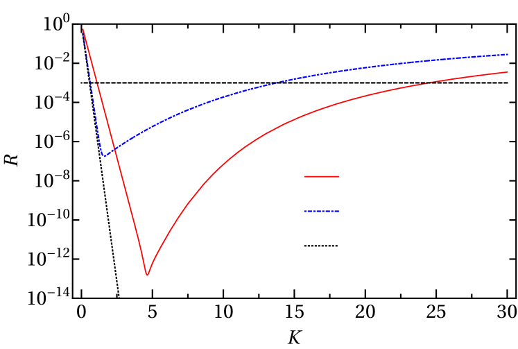
In Table 2, we list the optimal parameters we have found for our , , and . The table includes the resulting values of , and we expect that they are the optimal values to within a few percent. Note that we used =0.1 for the M-JWKB CAP based on the solution of taken from Fig. 3 of Ref. Manolopoulos (2002). We show in Fig. 10 the corresponding reflection coefficients.
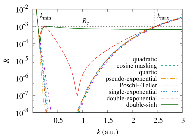
The cosine masking function should be regarded as a polynomial CAP since its behavior in for the optimal parameters of Table 2 is largely indistinguishable from the quadratic CAP — thus its is identical to the quadratic CAP. Similarly, for the optimal parameters we found, only the exponential tail of the Pöschl-Teller potential remained on the grid, making its performance essentially identical to that of the purely imaginary single-exponential CAP.
The absorption ranges listed in Table 2 display a surprisingly large range — more than a factor of 4. Comparing only the purely imaginary potentials, the exponential and Pöschl-Teller forms are more than 30% more efficient than the quadratic CAP. They are also more efficient than the quartic CAP. So, while the exponential form generally seems better, the majority of the disparity in Table 2 arises from adding a real part to the CAP and imposing a complex boundary condition.
From Table 2, the best performance is found for the double-exponential and double-sinh CAPs, outperforming the next-best CAP — the complex-valued, complex-boundary-condition, single-exponential CAP — by roughly 40%. Compared to the next-best purely imaginary CAP, they hold nearly a factor of 3 advantage in . For reference, we tested the strategy of adding a real part and a complex boundary condition to the quadratic CAP and found shrank only to about 70 a.u. So, while pursuing this strategy with the other CAPs in the table would reduce their , we believe the double-exponential and double-sinh CAPs would remain the best. Interestingly, since the de Broglie wavelength at is 57 a.u., our best CAP manages its efficient absorption in a range of only about half this longest wavelength.
Our recommendation, therefore, is to use the double-sinh CAP when its singularity at the boundary causes no numerical difficulties. In the cases that it does, then the double-exponential CAP is the best choice. The remainder of our discussion will thus focus on these two CAPs.
V Other absorption criteria
The discussion and optimization so far has centered on the , , and from Eq. (3). Other choices may well be needed, however, for other choices of laser parameters or calculational goals. We thus present in this section the optimal parameters for the double-exponential and double-sinh CAPs for a selection of likely changes in , , and .
V.1 Different energy range
V.1.1 Changing
Computationally, the main challenges in solving the TDSE — especially for current and future laser parameters of experimental interest — are that in the course of its strongly-driven dynamics, the electron travels far from the nucleus and gains substantial energy. In particular, we still expect , so that it will grow either with increasing intensity or increasing wavelength — both of which are certainly of interest. While does not change in this case, does, and the CAP must accommodate it.
Under these conditions, the double-sinh CAP from Table 2 works without change since it has no . In fact, this is its primary advantage. The double-exponential CAP, on the other hand, must be re-optimized for each . As discussed in Sec. II, needs the greatest changes — but should have minimal impact on — and these expectations are reflected in the optimal parameters shown in Table 3 for two longer wavelengths. These parameters were found following the same procedure as above with the same and and with = at W/cm2. They were found assuming on the boundary, but parameters could certainly be found for a complex boundary condition as well. Note that changes less than about 10% as expected.
| (nm) | ||||||
|---|---|---|---|---|---|---|
| 800 | 0.006 | 3 | 0.839 | 5.09 | 1.79 | 29.9 |
| 1600 | 0.006 | 8.8 | 1.07 | 8.37 | 1.79 | 30.7 |
| 2400 | 0.006 | 20 | 1.31 | 12.4 | 1.79 | 31.5 |
V.1.2 Changing
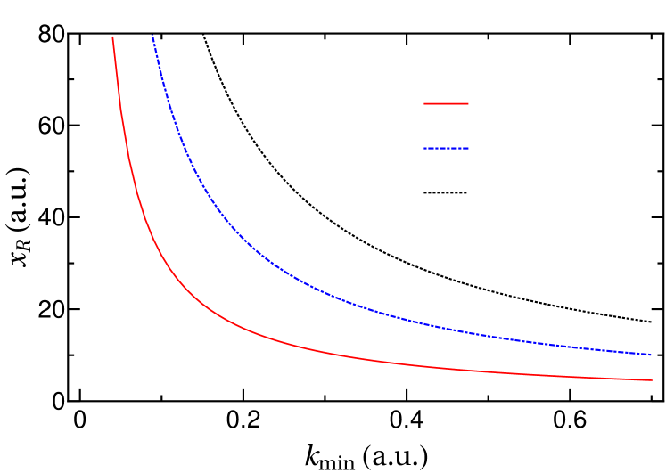
In our optimization scheme above, we set to 0.1 for 800-nm light. This choice was motivated by the need to ensure that the entire ionized electron wavepacket is absorbed by the CAP. However, the CAP is often placed at a large distance from the nucleus so that these very slow electrons may not have time to reach the CAP during the propagation. In this case, can be increased, thereby decreasing .
Modifications to for the double-sinh CAP are straightforward and do not require re-optimization — again, thanks to the lack of an . Changing just means recalculating using since is fixed. Figure 11 shows the that results as a function of . The figure shows that for modest increases in from our choice in Eq. (4), can be decreased substantially. For example, for above about 0.3 a.u., is smaller than 10 a.u. for =. For above about 0.4 a.u., the for = is equal to or smaller than the original =28.8 a.u. for the double-sinh CAP.
For a double-exponential CAP, it is still true that the larger , the smaller and , and the smaller . However, re-optimization is required to obtain the smallest . For instance, if one can accept doubling to 0.22 a.u., then we can have
| (24) |
with =0.90 a.u.
On the other hand, the double-exponential CAP can be adjusted just like the double-sinh CAP if a less-than-optimal can be tolerated. Specifically, the values of can be kept, so that does not change, and can be recalculated from . In this case, grows to , guaranteeing absorption at the prescribed level beyond . The resulting looks very much like those in Fig. 11, except that for = does not go below 10 a.u. until =0.45 a.u. For comparison, =17.4 a.u. at =0.22 a.u. and is thus slightly worse than the fully re-optimized result in Eq. (24).
V.2 Different
One of the primary design goals of a CAP is to leave the physical wave function — the wave function outside the absorption region — unaffected. Of course, this goal can only be achieved to a given accuracy, and that accuracy is controlled by . To see the relation, consider the physical wave function written in Fig. 1 from which is extracted,
| (25) |
The second term is precisely the unwanted contribution from reflection, and it is limited by by design. Given that this is just one component of the time-dependent wave function, this error is always relative to the first term. In other words, if one desires digits to be accurate, then one should choose =.
We thus provide in Table 4 the optimal parameters for the double-exponential and double-sinh CAPs with =0 on the boundary, assuming =0.006 a.u. and =3 a.u. as before, for several smaller . These results show that the absorption range for each type of CAP is comparable, with the double-sinh CAP tending to be a few percent smaller. Qualitatively, the reflection coefficients as a function of resemble those shown previously for =. As with the other CAP parameters we have given, we expect these to produce within a few percent of the global optimum.
| Double exponential | Double sinh | |||||||
|---|---|---|---|---|---|---|---|---|
| (a.u.) | (a.u.) | (a.u.) | (a.u.) | |||||
| 2.69 | 16.3 | 1.79 | 29.9 | 28.8 | 1.97 | |||
| 2.77 | 44.7 | 40.4 | 2.90 | |||||
| 3.38 | 54.5 | 52.6 | 3.87 | |||||
| 80.0 | 4.02 | 68.4 | 64.2 | 4.77 | ||||
| 6.64 | 102 | 89.4 | 6.77 | |||||
| 8.48 | 130 | 109 | 8.02 | |||||
| 48 | 9.04 | 144 | 132 | 9.77 | ||||
Note that the probability density corresponding to the wave function in Eq. (25),
| (26) |
can be useful for diagnosing issues with the CAP in a time-dependent calculation. In particular, the last term above is the source of the telltale ripples in the probability density near the edge of a grid. The ripples’ size is limited by and identifying their wavelength via Eq. (26) in a time-dependent wave function reveals the offending energy.
VI Time-Dependent Demonstration
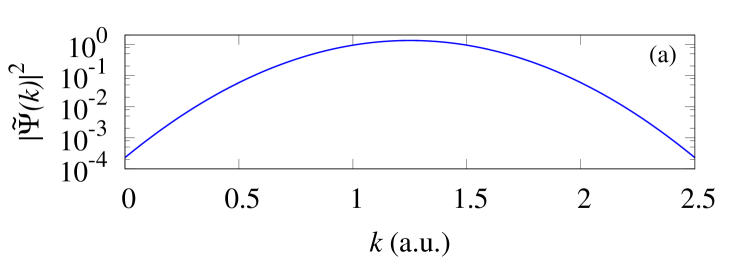
To verify that the improved performance of our recommended CAPs does indeed carry over to the time-dependent problem and its numerical solution, we solve the TDSE for free-electron wavepacket propagation. The wavepacket we use possesses a broad momentum distribution comparable to the target momentum range from Eq. (4), as shown in Fig. 12(a).
We again use FEDVR as the spatial representation and propagate the wave function using the short-time evolution operator
| (27) |
where the Hamiltonian includes the CAP ,
| (28) |
and is merely the kinetic energy in the present case. We evaluate using the split-operator form Schneider et al. (2011)
| (29) |
Since is diagonal in FEDVR, can be easily evaluated and applied. Moreover, in this form, the singularity in the double-sinh CAP causes no problems whatsoever. The action of the remaining term in is calculated via a Padé approximation Blanes et al. (2009).
Equation (29) is a simple and convenient way to add a CAP to any propagator. In many cases, the alternative, keeping the CAP in , would require modifications of the propagation algorithm or parameters to handle its non-Hermiticity or the singularity of the double-sinh CAP — or both. These issues were discussed somewhat in Sec. III.3 and more in Ref. Manolopoulos (2002). Using Eq. (29) avoids these concerns and is more than sufficient for the application of the CAP.
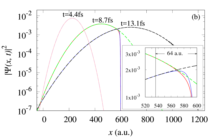
The FEDVR element distribution is uniform in the range , and we require at the boundaries. Given that the wavepacket is initially centered near , this box is large enough for the wavepacket to propagate for 10 fs without significant reflection at the boundaries even without CAPs. This will be our reference solution. We carry out a second, identical propagation but apply the double-sinh CAP at . For this example, we choose the CAP designed to have using the parameters shown in Table 4. We thus compare the wavepacket with and without applying the CAP. All the results have been tested to be converged to at least 3 digits with respect to all numerical parameters.
Figure 12 shows the two wavepackets at different times. It is clear that the CAP is performing as expected since the wavepacket decays in the absorbing region without any of the characteristic oscillations of reflections visible — at least without enlarging the plot by a factor of four or five. For comparison, the wavepacket without a CAP equally clearly shows the reflection oscillations at =13.1 fs for reflections from the boundary at =1200 a.u.
In addition, the with-CAP wavepacket is numerically unaffected before entering the absorbing region, agreeing with the without-CAP wavepacket to at least 3 digits for a.u. for all times, even as more than 70% of the wavepacket has been absorbed. This agreement shows that the absorption range defined in the time-independent study is consistent with the results from the time-dependent propagation.
Enlarging Fig. 12 by a factor of at least four or five will reveal the tiny reflection ripples in the with-CAP wavepacket near and in the absorption region. Their relative magnitude is about = as expected. Per the discussion in Sec. V.2, such oscillations are unavoidable with a CAP and testing with other CAPs and values of further support the conclusions there. For example, the oscillation for = becomes fairly noticeable, which suggests that should in practice be no larger than — i.e., two digits in the wave function — to provide quantitatively reliable results. Finally, we note that the roughly 15-fs propagation time is comparable to a typical strong-field calculation, bringing some realism to this simple demonstration.
VII Summary
We have presented a systematic study to boost the performance of complex absorbing potentials. Based on the time-independent reflection coefficient, we were able to quantitatively design the most optimal absorbing potential of a given form. In particular, for ultrafast, strong-field TDSE solvers, the optimal CAP parameters should be determined by the absorbing energy range required for the laser parameters and by the desired accuracy of the TDSE solutions.
We proposed two new CAPs — namely, the double-sinh CAP and the double-exponential CAP — that significantly outperform the CAPs currently in standard use. Their superiority was demonstrated through comparison with optimized versions of most of the CAPs commonly found in the literature. Both of our proposed CAPs overcome the primary impediment to efficient performance — absorption of long wavelengths — while also absorbing a large range of energies that covers basically all strong-field processes. Because we quantified the CAP’s performance and identified as the figure of merit for their efficiency, we could show that using an exponential CAP already improved on the common quadratic CAP’s performance by one third. A further factor of almost three was gained, however, by adding a real part to the CAP — a strategy well known in other uses of CAPs, but not in strong-field applications.
We highly recommend the double-sinh CAP for local spatial representations, such as FEDVR where the potential is diagonal. It is efficient, easy to use, and easy to adapt to different absorption criteria — i.e., energy range and level of absorption. Incorporating it into the time propagation via split-operator methods is easy and effective.
For other spatial representations, the double-sinh and the double-exponential CAPs are equally recommended. However, care might need to be taken for the double-sinh singularity close to the boundary. In case the double-sinh singularity is a problem for the propagator, the double-exponential CAP should be chosen. Although optimization of the double-exponential CAP is more involved than for the double-sinh CAP, it is still fairly straightforward. Its optimization procedure, along with that for the double-sinh CAP, is detailed in this work.
Appendix A Reflection Coefficient for Single-Exponential CAP
We start from the Schrödinger equation for the single-exponential CAP:
| (30) |
Setting gives
| (31) |
where and . We define
so that Eq. (31) becomes
| (32) |
This is Bessel’s equation; the general solution is thus
| (33) |
To obtain the reflection coefficient, we need and and we need to analyze the asymptotic behavior of these solutions. Starting with the latter, the () behavior can be found from the expansions,
| (34) |
To find and , we impose the boundary condition,
| (35) |
Thus,
| (36) |
Finally, the asymptotic solution reads
| (37) |
From this expression, the reflection coefficient can be found to be
| (38) |
Note that if is real, then as it should with no absorption.
Appendix B Reflection Coefficient for Double-Exponential CAP
As in App. A, we start from a unitless Schrödinger equation,
| (39) |
with
| (40) |
We assume both are real, making the longer-range potential real in accord with the discussion in the text. That is, the real potential accelerates the wave before it encounters the absorbing potential.
Defining
| (41) |
we get
| (42) |
This form of the equation makes clear the motivation for our choice of potential: having one potential being the square of the other (in form) produces the polynomial in seen in the equation. Since the polynomial is quadratic, the equation has analytic solutions.
Setting and , the solution can be written as
| (43) |
where and are the confluent hypergeometric and Laguerre functions, respectively.
Analyzing the asymptotic behavior, we have
| (44) |
The boundary condition gives
| (45) |
The reflection coefficient can now be extracted, and a little algebra applied, to give
| (46) |
For a purely real (i.e., ), we recover as we should. For , reduces to the single-exponential expression Eq. (38) with purely imaginary.
Appendix C Complex boundary condition
C.1 Zero potential
It is easiest to understand the effect of the complex boundary condition ( is complex)
| (47) |
from the free-particle equation
| (48) |
in the same unitless notation as in the previous appendices. In this notation, we must require
| (49) |
where . The solution is, as usual,
| (50) |
When combined with the boundary condition, one finds
| (51) |
As discussed in the text, this goes to zero at when . Physically, this condition corresponds to setting an outgoing-wave boundary condition (on the left boundary) for an incident momentum . The boundary is thus perfectly transparent at this momentum, but imperfectly so at other momenta.
C.2 Effect on bound states
It is natural to ask what effect such a boundary condition might have on the energies of any bound states in the system. One general way to answer this question is to consider an arbitrary potential at and write
| (52) |
with and the energy-dependent solution appropriate to the arbitrary potential satisfying the required boundary condition at . Although this specific description assumes a short-range potential, a similar argument can be made for the Coulomb potential.
The wave function in Eq. (52) must satisfy the log-derivative boundary condition from Eq. (49) at — this is why the exponentially-growing solution must be retained. Imposing this boundary condition leads to the following transcendental equation for the energy of the bound state:
| (53) |
This equation should be compared with the physical quantization condition
| (54) |
to which Eq. (53) reduces in the limit as it should.
Since in any practical numerical solution of the TDSE the boundary of the numerical grid must be large compared to the size of the bound state, we will have . Therefore, so long as , the exponential term on the right-hand-side of Eq. (53) will dominate — and thus make Eq. (53) a very good approximation to Eq. (54) — guaranteeing that the real part of the energy found with the complex boundary condition will be very close to the physical energy. To be sure, it will acquire a small imaginary part reflecting the decay of the ground state due to the complex boundary condition, but it should be completely negligible.
This result for the bound-state energies is completely consistent with the intuitive notion that the effect of the complex boundary condition — indeed the CAPs, too — on the bound states should be negligible so long as the bound-state wave function is vanishingly small at the boundary (or in the absorbing region of the CAP).
C.3 Single- and double-exponential CAPs
The reflection coefficient for the single-exponential CAP with a complex boundary condition is still analytical. It is found by imposing Eq. (49) on the general solution for the single-exponential CAP from Eq. (33). After a little algebra, one obtains
| (55) |
The same procedure can be carried out for the double-exponential CAP using the general solution from Eq. (43) to find
| (56) |
Appendix D Reflection Coefficient for CAP
We start from the Schrödinger equation
| (57) |
Defining , we must solve
| (58) |
The general solution is
| (59) |
with = as before. Since we require =0, we need the small- behavior of the Bessel functions
| (60) |
For the general case of complex , , one can show that requiring the real part of the potential to be attractive and the imaginary part to be absorbing leads to
| (61) |
These conditions, together with Eq. (60), require us to set =0.
Finally, using the large- behavior of the Bessel function,
| (62) |
allows us to extract the reflection coefficient,
| (63) |
Keeping in mind that under the conditions we have assumed, this equation shows that both the real and imaginary parts of the CAP contribute to decreasing the final absorption. We also see that this equation is identical to Eq. (20) once the conversion from to is made.
Effect of truncation
If we are willing to sacrifice the energy independence of at small energies by truncating the CAP at ,
| (64) |
then one can again obtain an analytic expression for the reflection coefficient.
The wave function is
| (65) |
with and . The reflection coefficient is thus
| (66) |
The notation indicates a derivative with respect to , , and the log-derivative of at is
| (67) |
A plot of the reflection coefficient from Eq. (66) looks qualitatively like the double-sinh reflection coefficients in Figs. 7 and 10. However, instead of falling exponentially with at small , it falls more slowly — like . In addition, because of the sharp cutoff in the potential, oscillates in with minima separated by at positions corresponding roughly to .
Acknowledgements.
This work is supported by the Chemical Sciences, Geoscience, and Biosciences Division, Office for Basic Energy Sciences,Office of Science, U.S. Department of Energy.References
- Heather and Metiu (1987) R. Heather and H. Metiu, The Journal of Chemical Physics 86, 5009 (1987), http://dx.doi.org/10.1063/1.452672 .
- Tao and Scrinzi (2012) L. Tao and A. Scrinzi, New Journal of Physics 14, 013021 (2012).
- Morales et al. (2016) F. Morales, T. Bredtmann, and S. Patchkovskii, Journal of Physics B: Atomic, Molecular and Optical Physics 49, 245001 (2016).
- Kosloff and Kosloff (1986) R. Kosloff and D. Kosloff, Journal of Computational Physics 63, 363 (1986).
- Vibok and Balint-Kurti (1992a) A. Vibok and G. G. Balint-Kurti, The Journal of Chemical Physics 96, 7615 (1992a).
- Vibok and Balint-Kurti (1992b) A. Vibok and G. G. Balint-Kurti, The Journal of Physical Chemistry 96, 8712 (1992b).
- Macias et al. (1994) D. Macias, S. Brouard, and J. Muga, Chemical Physics Letters 228, 672 (1994).
- Riss and Meyer (1996) U. V. Riss and H. Meyer, The Journal of Chemical Physics 105, 1409 (1996).
- Ge and Zhang (1998) J.-Y. Ge and J. Z. H. Zhang, The Journal of Chemical Physics 108, 1429 (1998).
- Hussain and Roberts (2000) A. N. Hussain and G. Roberts, Phys. Rev. A 63, 012703 (2000).
- Manolopoulos (2002) D. E. Manolopoulos, The Journal of Chemical Physics 117, 9552 (2002), http://dx.doi.org/10.1063/1.1517042 .
- Poirier and Carrington (2003) B. Poirier and T. Carrington, The Journal of Chemical Physics 119, 77 (2003).
- Muga et al. (2004) J. Muga, J. Palao, B. Navarro, and I. Egusquiza, Physics Reports 395, 357 (2004).
- Tarana and Greene (2012) M. Tarana and C. H. Greene, Phys. Rev. A 85, 013411 (2012).
- Strelkov et al. (2012) V. V. Strelkov, M. A. Khokhlova, A. A. Gonoskov, I. A. Gonoskov, and M. Y. Ryabikin, Phys. Rev. A 86, 013404 (2012).
- Yue and Madsen (2013) L. Yue and L. B. Madsen, Phys. Rev. A 88, 063420 (2013).
- Krause et al. (2014) P. Krause, J. A. Sonk, and H. B. Schlegel, The Journal of Chemical Physics 140, 174113 (2014).
- Krause et al. (1992) J. L. Krause, K. J. Schafer, and K. C. Kulander, Phys. Rev. A 45, 4998 (1992).
- Rescigno et al. (1999) T. N. Rescigno, M. Baertschy, W. A. Isaacs, and C. W. McCurdy, Science 286, 2474 (1999).
- Rescigno and McCurdy (2000) T. N. Rescigno and C. W. McCurdy, Phys. Rev. A 62, 032706 (2000).
- He et al. (2007) F. He, C. Ruiz, and A. Becker, Phys. Rev. A 75, 053407 (2007).
- Tao et al. (2009) L. Tao, W. Vanroose, B. Reps, T. N. Rescigno, and C. W. McCurdy, Phys. Rev. A 80, 063419 (2009).
- Scrinzi (2010) A. Scrinzi, Phys. Rev. A 81, 053845 (2010).
- Sidky and Esry (2000) E. Y. Sidky and B. D. Esry, Phys. Rev. Lett. 85, 5086 (2000).
- Hamido et al. (2011) A. Hamido, J. Eiglsperger, J. Madroñero, F. Mota-Furtado, P. O’Mahony, A. L. Frapiccini, and B. Piraux, Phys. Rev. A 84, 013422 (2011).
- Miyagi and Madsen (2016) H. Miyagi and L. B. Madsen, Phys. Rev. A 93, 033420 (2016).
- Zhang (1990) J. Z. H. Zhang, The Journal of Chemical Physics 92, 324 (1990), http://dx.doi.org/10.1063/1.458433 .
- Williams et al. (1991) C. J. Williams, J. Qian, and D. J. Tannor, The Journal of Chemical Physics 95, 1721 (1991), http://dx.doi.org/10.1063/1.461022 .
- Yao and Chu (1992) G. H. Yao and S. I. Chu, Chem. Phys. Lett. 198, 39 (1992).
- Yoshida et al. (1999) S. Yoshida, S. Watanabe, C. O. Reinhold, and J. Burgdörfer, Phys. Rev. A 60, 1113 (1999).
- McCurdy et al. (2001) C. W. McCurdy, D. A. Horner, and T. N. Rescigno, Phys. Rev. A 63, 022711 (2001).
- Schneider et al. (2006) B. I. Schneider, L. A. Collins, and S. X. Hu, Phys. Rev. E 73, 036708 (2006).
- Aymar et al. (1996) M. Aymar, C. H. Greene, and E. Luc-Koenig, Rev. Mod. Phys. 68, 1015 (1996).
- Pöschl and Teller (1933) G. Pöschl and E. Teller, Zeitschrift fur Physik 83, 143 (1933).
- Landau and Lifshitz (1977) L. D. Landau and E. M. Lifshitz, Quantum Mechanics: Non-Relativistic Theory (Pergamon Press, 1977).
- Schneider et al. (2011) B. I. Schneider, J. Feist, S. Nagele, R. Pazourek, S. Hu, L. A. Collins, and J. Burgdörfer, in Quantum Dynamic Imaging: Theoretical and Numerical Methods, edited by A. D. Bandrauk and M. Ivanov (Springer Science & Business Media, 2011).
- Blanes et al. (2009) S. Blanes, F. Casas, J. Oteo, and J. Ros, Physics Reports 470, 151 (2009).