This paper was converted on www.awesomepapers.org from LaTeX by an anonymous user.
Want to know more? Visit the Converter page.

Analysis of a dynamic viscoelastic-viscoplastic piezoelectric contact problem

M. Campo J.R. Fernández Á. Rodríguez-Arós J.M. Rodríguez Centro Universitario de la Defensa, Escuela Naval Militar
Plaza de España s/n, 36920 Marín, Spain
Departamento de Matemática Aplicada I, Universidade de Vigo
Escola de Enxeñería de Telecomunicación, Campus As Lagoas Marcosende s/n, 36310 Vigo, Spain
Departamento de Métodos Matemáticos e Representación
Universidade de A Coruña, A Coruña, Spain
Corresponding author: Phone: +34986818746. Fax: +34986812116. E-mail address: jose.fernandez@uvigo.es
Abstract

In this paper, we study, from both variational and numerical points of view, a dynamic contact problem between a viscoelastic-viscoplastic piezoelectric body and a deformable obstacle. The contact is modelled using the classical normal compliance contact condition. The variational formulation is written as a nonlinear ordinary differential equation for the stress field, a nonlinear hyperbolic variational equation for the displacement field and a linear variational equation for the electric potential field. An existence and uniqueness result is proved using Gronwall’s lemma, adequate auxiliary problems and fixed-point arguments. Then, fully discrete approximations are introduced using an Euler scheme and the finite element method, for which some a priori error estimates are derived, leading to the linear convergence of the algorithm under suitable additional regularity conditions. Finally, some two-dimensional numerical simulations are presented to show the accuracy of the algorithm and the behaviour of the solution.

Keywords. Viscoelasticity, viscoplasticity, piezoelectricity, existence and uniqueness, a priori error estimates, numerical simulations.

1 Introduction

Dynamic contact problems for viscoelastic materials have been studied in numerous publications. For instance, we could refer the papers [12, 18, 20, 19, 31, 32, 35, 36, 37, 40, 44] where these problems were considered assuming different friction laws and types of contact (deformable and rigid obstacles or bilateral contact, Coulomb’s friction law, slip dependent friction, etc). Moreover, the numerical approximation of these problems were also done, including effects as the adhesion, the piezoelectricity or the damage (see, e.g., [1, 2, 4, 7, 13, 14, 21, 22, 26]).

These viscoelastic materials have been utilized in many engineering applications since they can be customized to meet a desired performance while maintain low cost. An important issue concerning such materials is that they may exhibit time-dependent and inelastic deformations. The viscoelastic strain component consists of a recoverable-reversible part (elastic strain) and a recoverable-dissipative deformation part (inelastic strain). When an inelastic strain is assumed to depend only on the magnitude of the stress or strain, the term plastic strain is used. When the plastic deformation also changes with time, like in the viscous component of the viscoelastic part, the term viscoplastic strain is used. Therefore, a combined viscoelastic-viscoplastic constitutive relationships should be considered. Recently, new models coupling both viscoplastic and viscoelastic effects have been proposed (see, for instance, [3, 10, 15, 16, 27, 29, 33, 39, 41]).

Piezoelectricity is the ability of certain cristals, like the quartz (also ceramics (BaTiO3, KNbO3, LiNbO3, PZT-5A, etc.) and even the human mandible or the human bone), to produce a voltage when they are subjected to mechanical stress. This effect is characterized by the coupling between the mechanical and the electrical properties of the material. We note that this kind of materials appears usually in the industry as switches in radiotronics, electroacoustics or measuring equipments. Since the first studies by Toupin ([47, 48]) and Mindlin ([42, 43]) a large number of papers have been published dealing with related models (see, for instance, [30, 11, 45] and the references cited therein). During the last ten years, numerous contact problems involving this piezoelectric effect have been studied from the variational and numerical points of view (see, i.e., [6, 7, 8, 44, 37, 38]).

In this paper, the contact is assumed to be with a deformable obstacle and so, the classical normal compliance contact condition is used ([34, 40]). Moreover, a viscoelastic-viscoplastic material is considered including, for the sake of generality in the modelling, piezoelectric effects. Both variational and numerical analyses are then performed, providing the existence of a unique weak solution to the continuous problem and an a priori error analysis for the fully discrete approximations. Finally, some numerical simulations are presented in two-dimensional examples to demonstrate the accuracy of the approximation and the behaviour of the solution.

The outline of this paper is as follows. In Section 2, we describe the mathematical problem and derive its variational formulation. An existence and uniqueness result is proved in Section 3. Then, fully discrete approximations are introduced in Section 4 by using the finite element method for the spatial approximation and an Euler scheme for the discretization of the time derivatives. An error estimate result is proved from which the linear convergence is deduced under suitable regularity assumptions. Finally, in Section 5 some two-dimensional numerical examples are shown to demonstrate the accuracy of the algorithm and the behaviour of the solution.

2 Mechanical problem and its variational formulation

Denote by 𝕊d\mathbb{S}^{d}, d=1,2,3d=1,2,3, the space of second order symmetric tensors on d\mathbb{R}^{d} and by “\cdot” and \|\cdot\| the inner product and the Euclidean norms on d\mathbb{R}^{d} and 𝕊d\mathbb{S}^{d}.

Let Ωd\Omega\subset\mathbb{R}^{d} denote a domain occupied by a viscoelastic-viscoplastic piezoelectric body with a Lipschitz boundary Γ=Ω\Gamma=\partial\Omega decomposed into three measurable parts ΓD\Gamma_{D}, ΓF\Gamma_{F}, ΓC\Gamma_{C}, on one hand, and on two measurable parts ΓA\Gamma_{A} and ΓB\Gamma_{B}, on the other hand, such that meas (ΓD)>0\hbox{meas }(\Gamma_{D})>0, meas (ΓA)>0\hbox{meas }(\Gamma_{A})>0, and ΓCΓB\Gamma_{C}\subseteq\Gamma_{B}. Let [0,T][0,T], T>0T>0, be the time interval of interest. The body is being acted upon by a volume force with density 𝒇0\mbox{\boldmath{$f$}}_{0}, it is clamped on ΓD\Gamma_{D} and surface tractions with density 𝒇F\mbox{\boldmath{$f$}}_{F} act on ΓF\Gamma_{F}. Moreover, an electrical potential is prescribed on ΓA\Gamma_{A} and electric charges are applied on ΓB\Gamma_{B}. Finally, we assume that the body may come in contact with a deformable obstacle on the boundary part ΓC\Gamma_{C}, which is located, in its reference configuration, at a distance ss, measured along the outward unit normal vector 𝝂=(νi)i=1d\mbox{\boldmath{$\nu$}}=(\nu_{i})_{i=1}^{d}.

Let 𝒙Ω\mbox{\boldmath{$x$}}\in\Omega and t[0,T]t\in[0,T] be the spatial and time variables, respectively. In order to simplify the writing, some times we do not indicate the dependence of various functions and unknowns on 𝒙x and tt. Moreover, a dot above a variable represents its first derivative with respect to the time variable and two dots indicate derivative of the second order.

Let 𝒖=(ui)i=1dd\mbox{\boldmath{$u$}}=(u_{i})_{i=1}^{d}\in\mathbb{R}^{d}, φ\varphi\in\mathbb{R}, 𝝈=(σij)i,j=1d𝕊d\mbox{\boldmath{$\sigma$}}=(\sigma_{ij})_{i,j=1}^{d}\in\mathbb{S}^{d} and 𝜺(𝒖)=(εij(𝒖))i,j=1d𝕊d\mbox{\boldmath{$\varepsilon$}}(\mbox{\boldmath{$u$}})=(\varepsilon_{ij}(\mbox{\boldmath{$u$}}))_{i,j=1}^{d}\in\mathbb{S}^{d} denote the displacements, the electric potential, the stress tensor and the linearized strain tensor, respectively. We recall that

εij(𝒖)=12(uixj+ujxi),i,j=1,,d.\varepsilon_{ij}(\mbox{\boldmath{$u$}})=\frac{1}{2}\left(\frac{\partial u_{i}}{\partial x_{j}}+\frac{\partial u_{j}}{\partial x_{i}}\right),\quad i,j=1,\ldots,d.

The body is assumed to be made of a viscoelastic-viscoplastic piezoelectric material and it satisfies the following constitutive law (see, for instance, [23, 30]),

𝝈(𝒙,t)=𝒜𝜺(𝒖˙(𝒙,t))+𝜺(𝒖(𝒙,t))+0t𝒢(𝝈(𝒙,s),𝜺(𝒖(𝒙,s)))𝑑s𝐄(φ(𝒙,t)),\begin{array}[]{l}\displaystyle\mbox{\boldmath{$\sigma$}}(\mbox{\boldmath{$x$}},t)=\mathcal{A}\mbox{\boldmath{$\varepsilon$}}(\dot{\mbox{\boldmath{$u$}}}(\mbox{\boldmath{$x$}},t))+\mathcal{B}\mbox{\boldmath{$\varepsilon$}}(\mbox{\boldmath{$u$}}(\mbox{\boldmath{$x$}},t))+\int_{0}^{t}\mathcal{G}(\mbox{\boldmath{$\sigma$}}(\mbox{\boldmath{$x$}},s),\mbox{\boldmath{$\varepsilon$}}(\mbox{\boldmath{$u$}}(\mbox{\boldmath{$x$}},s)))\,ds\\ \qquad\qquad-\mathcal{E}^{*}{\bf E}(\varphi(\mbox{\boldmath{$x$}},t)),\end{array} (2.1)

where 𝒜=(aijkl)\mathcal{A}=(a_{ijkl}) and =(bijkl)\mathcal{B}=(b_{ijkl}) are the fourth-order viscous and elastic tensors, respectively, 𝒢\mathcal{G} is a viscoplastic function whose properties will be detailed later, 𝐄(φ)=(Ei(φ))i=1d{\bf E}(\varphi)=(E_{i}(\varphi))_{i=1}^{d} represents the electric field defined by

Ei(φ)=φxi,i=1,,d,E_{i}(\varphi)=-\frac{\partial\varphi}{\partial x_{i}},\quad i=1,\ldots,d,

and =(eijk)i,j,k=1d\mathcal{E}^{*}=(e_{ijk}^{*})_{i,j,k=1}^{d} denotes the transpose of the third-order piezoelectric tensor =(eijk)i,j,k=1d\mathcal{E}=(e_{ijk})_{i,j,k=1}^{d}. We recall that

eijk=ekij,for alli,j,k=1,,d.e_{ijk}^{*}=e_{kij},\quad\hbox{for all}\quad i,j,k=1,\ldots,d.

Following [11] the following constitutive law is satisfied for the electric potential,

𝒟=𝜺(𝒖)+β𝐄(φ),\mathcal{D}=\mathcal{E}\mbox{\boldmath{$\varepsilon$}}(\mbox{\boldmath{$u$}})+\mathbf{\beta}{\bf E}(\varphi),

where 𝒟=(Di)i=1d\mathcal{D}=(D_{i})_{i=1}^{d} is the electric displacement field and β=(βij)i,j=1d\mathbf{\beta}=(\beta_{ij})_{i,j=1}^{d} is the electric permittivity tensor.

We turn now to describe the boundary conditions.

On the boundary part ΓD\Gamma_{D} we assume that the body is clamped and thus the displacement field vanishes there (and so 𝒖=𝟎\mbox{\boldmath{$u$}}=\mbox{\boldmath{$0$}} on ΓD×(0,T)\Gamma_{D}\times(0,T)). Moreover, since the density of traction forces 𝒇F\mbox{\boldmath{$f$}}_{F} is applied on the boundary part ΓF\Gamma_{F}, it follows that 𝝈𝝂=𝒇F\mbox{\boldmath{$\sigma$}}\mbox{\boldmath{$\nu$}}=\mbox{\boldmath{$f$}}_{F} on ΓF×(0,T).\Gamma_{F}\times(0,T).

The contact is assumed with a deformable obstacle and so, the well-known normal compliance contact condition is employed for its modeling (see [34, 40]); that is, the normal stress σν=𝝈𝝂𝝂\sigma_{\nu}=\mbox{\boldmath{$\sigma$}}\mbox{\boldmath{$\nu$}}\cdot\mbox{\boldmath{$\nu$}} on ΓC\Gamma_{C} is given by

σν=p(uνs),-\sigma_{\nu}=p(u_{\nu}-s),

where uν=𝒖𝝂u_{\nu}=\mbox{\boldmath{$u$}}\cdot\mbox{\boldmath{$\nu$}} denotes the normal displacement, in such a way that, when uν>su_{\nu}>s, the difference uνsu_{\nu}-s represents the interpenetration of the body’s asperities into those of the obstacle. The normal compliance function pp is prescribed and it satisfies p(r)=0p(r)=0 for r0r\leq 0, since then there is no contact. As an example, one may consider

p(r)=cpr+,p(r)=c_{p}\,r_{+},

where cp>0c_{p}>0 represents a deformability constant (that is, it denotes the stiffness of the obstacle), and r+=max{0,r}.r_{+}={\rm max}\,\{0,r\}. Formally, the classical Signorini nonpenetration conditions are obtained in the limit cpc_{p}\to\infty. We also assume that the contact is frictionless, i.e. the tangential component of the stress field, denoted by 𝝈τ=𝝈𝝂σν𝝂\mbox{\boldmath{$\sigma$}}_{\tau}=\mbox{\boldmath{$\sigma$}}\mbox{\boldmath{$\nu$}}-\sigma_{\nu}\mbox{\boldmath{$\nu$}}, vanishes on the contact surface.

Let Ω\Omega be subject to a prescribed electric potential on ΓA\Gamma_{A} and to a density of surface electric charges qFq_{F} on ΓB\Gamma_{B}, that is,

φ=φAonΓA×(0,T),𝒟𝝂=qFonΓB×(0,T).\begin{array}[]{l}\varphi=\varphi_{A}\quad\hbox{on}\quad\Gamma_{A}\times(0,T),\\ \mathcal{D}\cdot\mbox{\boldmath{$\nu$}}=q_{F}\quad\hbox{on}\quad\Gamma_{B}\times(0,T).\end{array}

For the sake of simplicity, we assume that no electric potential is imposed on the boundary ΓA\Gamma_{A} (i.e. φA=0\varphi_{A}=0), and that qF=0q_{F}=0 on ΓC\Gamma_{C}; that is, the foundation is supposed to be insulator. We note that it is straightforward to extend the results presented below to more general situations by decomposing Γ\Gamma in a different way and by introducing some modifications in the analyses shown in the following sections.

The mechanical problem of the dynamic deformation of a viscoelastic-viscoplastic piezoelectric body in contact with a deformable obstacle is then written as follows.

Problem P. Find a displacement field 𝐮:Ω¯×[0,T]d\mbox{\boldmath{$u$}}:\overline{\Omega}\times[0,T]\rightarrow\mathbb{R}^{d}, a stress field 𝛔:Ω¯×[0,T]𝕊d\mbox{\boldmath{$\sigma$}}:\overline{\Omega}\times[0,T]\rightarrow\mathbb{S}^{d}, an electric potential field φ:Ω¯×(0,T)\varphi:\overline{\Omega}\times(0,T)\rightarrow\mathbb{R} and an electric displacement field 𝒟:Ω¯×(0,T)d\mathcal{D}:\overline{\Omega}\times(0,T)\rightarrow\mathbb{R}^{d} such that,

𝝈(𝒙,t)=𝒜𝜺(˙𝒖(𝒙,t))+𝜺(𝒖(𝒙,t))+0t𝒢(𝝈(𝒙,s),𝜺(𝒖(𝒙,s)))𝑑s\displaystyle\mbox{\boldmath{$\sigma$}}(\mbox{\boldmath{$x$}},t)=\mathcal{A}\mbox{\boldmath{$\varepsilon$}}(\dot{}\mbox{\boldmath{$u$}}(\mbox{\boldmath{$x$}},t))+\mathcal{B}\mbox{\boldmath{$\varepsilon$}}(\mbox{\boldmath{$u$}}(\mbox{\boldmath{$x$}},t))+\int_{0}^{t}\mathcal{G}(\mbox{\boldmath{$\sigma$}}(\mbox{\boldmath{$x$}},s),\mbox{\boldmath{$\varepsilon$}}(\mbox{\boldmath{$u$}}(\mbox{\boldmath{$x$}},s)))\,ds
𝐄(φ(𝒙,t))for a.e.𝒙Ω,t(0,T),\displaystyle\qquad\qquad-\mathcal{E}^{*}{\bf E}(\varphi(\mbox{\boldmath{$x$}},t))\quad\hbox{for a.e.}\quad\mbox{\boldmath{$x$}}\in\Omega,\,t\in(0,T), (2.2)
𝒟=𝜺(𝒖)+β𝐄(φ)inΩ×(0,T),\displaystyle\mathcal{D}=\mathcal{E}\mbox{\boldmath{$\varepsilon$}}(\mbox{\boldmath{$u$}})+\mathbf{\beta}{\bf E}(\varphi)\quad\hbox{in}\quad\Omega\times(0,T), (2.3)
ρ𝒖¨Div 𝛔=𝒇0inΩ×(0,T),\displaystyle\rho\ddot{\mbox{\boldmath{$u$}}}-\mbox{\rm Div\,}\mbox{\boldmath{$\sigma$}}=\mbox{\boldmath{$f$}}_{0}\quad\hbox{in}\quad\Omega\times(0,T), (2.4)
div 𝒟=q0inΩ×(0,T),\displaystyle\mbox{\rm div\,}\mathcal{D}=q_{0}\quad\hbox{in}\quad\Omega\times(0,T), (2.5)
𝒖=𝟎onΓD×(0,T),\displaystyle\mbox{\boldmath{$u$}}=\mbox{\boldmath{$0$}}\quad\hbox{on}\quad\Gamma_{D}\times(0,T), (2.6)
𝛔𝛎=𝒇FonΓF×(0,T),\displaystyle\mbox{\boldmath{$\sigma$}}\mbox{\boldmath{$\nu$}}=\mbox{\boldmath{$f$}}_{F}\quad\hbox{on}\quad\Gamma_{F}\times(0,T), (2.7)
𝝈τ=𝟎,σν=p(uνs)onΓC×(0,T),\displaystyle\mbox{\boldmath{$\sigma$}}_{\tau}=\mbox{\boldmath{$0$}},\quad-\sigma_{\nu}=p(u_{\nu}-s)\quad\hbox{on}\quad\Gamma_{C}\times(0,T), (2.8)
φ=0onΓA×(0,T),\displaystyle\varphi=0\quad\hbox{on}\quad\Gamma_{A}\times(0,T), (2.9)
𝒟𝝂=qFonΓB×(0,T),\displaystyle\mathcal{D}\cdot\mbox{\boldmath{$\nu$}}=q_{F}\quad\hbox{on}\quad\Gamma_{B}\times(0,T), (2.10)
𝒖(0)=𝒖0,𝒖˙(0)=𝒗0inΩ.\displaystyle\mbox{\boldmath{$u$}}(0)=\mbox{\boldmath{$u$}}_{0},\quad\dot{\mbox{\boldmath{$u$}}}(0)=\mbox{\boldmath{$v$}}_{0}\quad\hbox{in}\quad\Omega. (2.11)

Here, ρ>0\rho>0 is the density of the material (which is assumed constant for simplicity), and 𝒖0\mbox{\boldmath{$u$}}_{0} and 𝒗0\mbox{\boldmath{$v$}}_{0} represent initial conditions for the displacement and velocity fields, respectively. 𝒇0\mbox{\boldmath{$f$}}_{0} is the density of the body forces acting in Ω\Omega and q0q_{0} is the volume density of free electric charges. Moreover, Div  and div  represent the divergence operators for tensor and vector-valued functions, respectively.

In order to obtain the variational formulation of Problem P, let us denote by H=[L2(Ω)]dH=[L^{2}(\Omega)]^{d} and define the variational spaces VV, WW and QQ as follows,

V={𝒘[H1(Ω)]d;𝒘=𝟎onΓD},W={ψH1(Ω);ψ=0onΓA},Q={𝝉=(τij)i,j=1d[L2(Ω)]d×d;τij=τji,i,j=1,,d}.\begin{array}[]{l}V=\{\mbox{\boldmath{$w$}}\in[H^{1}(\Omega)]^{d}\,;\,\mbox{\boldmath{$w$}}=\mbox{\boldmath{$0$}}\quad\hbox{on}\quad\Gamma_{D}\},\\ W=\{\psi\in H^{1}(\Omega)\,;\,\psi=0\quad\hbox{on}\quad\Gamma_{A}\},\\ Q=\{\mbox{\boldmath{$\tau$}}=(\tau_{ij})_{i,j=1}^{d}\in[L^{2}(\Omega)]^{d\times d}\,\,\,;\,\,\,\tau_{ij}=\tau_{ji},\,\;i,j=1,\ldots,d\}.\end{array}
Remark 2.1

We could assume ρ\rho to be more general. To do that we should follow a standard procedure (see for example [46, p.105]). If we assume

ρL(Ω),ρ(𝒙)ρ>0a.e.𝒙Ω,\rho\in L^{\infty}(\Omega),\ \rho(\mbox{\boldmath{$x$}})\geq\rho^{*}>0\ {\rm a.e.}\ \mbox{\boldmath{$x$}}\in\Omega, (2.12)

where ρ\rho^{*} is a constant, we shall use a modified inner product in HH, given by

((𝒖,𝒗))H=Ωρ𝒖𝒗𝑑𝒙𝒖,𝒗H.((\mbox{\boldmath{$u$}},\mbox{\boldmath{$v$}}))_{H}=\int_{\Omega}\rho\mbox{\boldmath{$u$}}\cdot\mbox{\boldmath{$v$}}\,d\mbox{\boldmath{$x$}}\quad\forall\mbox{\boldmath{$u$}},\mbox{\boldmath{$v$}}\in H.

Let ||||||H|||\cdot|||_{H} denote the associated norm, i.e.,

|𝒖|H2=((𝒖,𝒖))H12𝒖H.|||\mbox{\boldmath{$u$}}|||_{H}^{2}=((\mbox{\boldmath{$u$}},\mbox{\boldmath{$u$}}))_{H}^{\frac{1}{2}}\quad\forall\mbox{\boldmath{$u$}}\in H.

By (2.12), the norm ||||||H|||\cdot|||_{H} is equivalent to the usual L2L^{2}-norm.

We will make the following assumptions on the problem data.

The viscosity tensor 𝒜(𝒙)=(aijkl(𝒙))i,j,k,l=1d:𝝉𝕊d𝒜(𝒙)(𝝉)𝕊d\mathcal{A}(\mbox{\boldmath{$x$}})=(a_{ijkl}(\mbox{\boldmath{$x$}}))_{i,j,k,l=1}^{d}:\mbox{\boldmath{$\tau$}}\in\mathbb{S}^{d}\rightarrow\mathcal{A}(\mbox{\boldmath{$x$}})(\mbox{\boldmath{$\tau$}})\in\mathbb{S}^{d} satisfies:

(a)aijkl=aklij=ajiklfori,j,k,l=1,,d.(b)aijklL(Ω)fori,j,k,l=1,,d.(c)Thereexistsm𝒜>0suchthat𝒜(𝒙)𝝉𝝉m𝒜𝝉2𝝉𝕊d,a.e.𝒙Ω.\begin{array}[]{l}\mathrm{(a)\ }a_{ijkl}=a_{klij}=a_{jikl}\quad\hbox{for}\quad i,j,k,l=1,\ldots,d.\\ \mathrm{(b)\ }a_{ijkl}\in L^{\infty}(\Omega)\quad\hbox{for}\quad i,j,k,l=1,\ldots,d.\\ \mathrm{(c)\ \mathrm{T}h\mathrm{ere}\ exists\ }m_{\mathcal{A}}>0\mathrm{\ such\ that\ }\mathcal{A}(\mbox{\boldmath{$x$}})\mbox{\boldmath{$\tau$}}\cdot\mbox{\boldmath{$\tau$}}\geq m_{\mathcal{A}}\,\|\mbox{\boldmath{$\tau$}}\|^{2}\\ {}\qquad\forall\,\mbox{\boldmath{$\tau$}}\in\mathbb{S}^{d},\mathrm{\ a.e.\ }\mbox{\boldmath{$x$}}\in\Omega.\end{array} (2.13)

The elastic tensor (𝒙)=(bijkl(𝒙))i,j,k,l=1d:𝝉𝕊d(𝒙)(𝝉)𝕊d\mathcal{B}(\mbox{\boldmath{$x$}})=(b_{ijkl}(\mbox{\boldmath{$x$}}))_{i,j,k,l=1}^{d}:\mbox{\boldmath{$\tau$}}\in\mathbb{S}^{d}\rightarrow\mathcal{B}(\mbox{\boldmath{$x$}})(\mbox{\boldmath{$\tau$}})\in\mathbb{S}^{d} satisfies:

(a)bijkl=bklij=bjiklfori,j,k,l=1,,d.(b)bijklL(Ω)fori,j,k,l=1,,d.(c)Thereexistsm>0suchthat(𝒙)𝝉𝝉m𝝉2𝝉𝕊d,a.e.𝒙Ω.\begin{array}[]{l}\mathrm{(a)\ }b_{ijkl}=b_{klij}=b_{jikl}\quad\hbox{for}\quad i,j,k,l=1,\ldots,d.\\ \mathrm{(b)\ }b_{ijkl}\in L^{\infty}(\Omega)\quad\hbox{for}\quad i,j,k,l=1,\ldots,d.\\ \mathrm{(c)\ \mathrm{T}h\mathrm{ere}\ exists\ }m_{\mathcal{B}}>0\mathrm{\ such\ that\ }\mathcal{B}(\mbox{\boldmath{$x$}})\mbox{\boldmath{$\tau$}}\cdot\mbox{\boldmath{$\tau$}}\geq m_{\mathcal{B}}\,\|\mbox{\boldmath{$\tau$}}\|^{2}\\ {}\qquad\forall\,\mbox{\boldmath{$\tau$}}\in\mathbb{S}^{d},\mathrm{\ a.e.\ }\mbox{\boldmath{$x$}}\in\Omega.\end{array} (2.14)

The piezoelectric tensor (𝒙)=(eijk(𝒙))i,j,k=1d:𝝉𝕊d(𝒙)(𝝉)d\mathcal{E}(\mbox{\boldmath{$x$}})=(e_{ijk}(\mbox{\boldmath{$x$}}))_{i,j,k=1}^{d}:\mbox{\boldmath{$\tau$}}\in\mathbb{S}^{d}\rightarrow\mathcal{E}(\mbox{\boldmath{$x$}})(\mbox{\boldmath{$\tau$}})\in\mathbb{R}^{d} satisfies:

(a)eijk=eikjfori,j,k=1,,d.(b)eijkL(Ω)fori,j,k=1,,d.\begin{array}[]{l}\mathrm{(a)\ }e_{ijk}=e_{ikj}\quad\hbox{for}\quad i,j,k=1,\ldots,d.\\ \mathrm{(b)\ }e_{ijk}\in L^{\infty}(\Omega)\quad\hbox{for}\quad i,j,k=1,\ldots,d.\end{array} (2.15)

The permittivity tensor β(𝒙)=(βij(𝒙))i,j=1d:𝒘dβ(𝒙)(𝒘)d\mathbf{\beta}(\mbox{\boldmath{$x$}})=(\beta_{ij}(\mbox{\boldmath{$x$}}))_{i,j=1}^{d}:\mbox{\boldmath{$w$}}\in\mathbb{R}^{d}\rightarrow\mathbf{\beta}(\mbox{\boldmath{$x$}})(\mbox{\boldmath{$w$}})\in\mathbb{R}^{d} verifies:

(a)βij=βjifori,j=1,,d.(b)βijL(Ω)fori,j=1,,d.(c)Thereexistsmβ>0suchthatβ(𝒙)𝒘𝒘mβ𝒘2𝒘d,a.e.𝒙Ω.\begin{array}[]{l}\mathrm{(a)\ }\beta_{ij}=\beta_{ji}\quad\hbox{for}\quad i,j=1,\ldots,d.\\ \mathrm{(b)\ }\beta_{ij}\in L^{\infty}(\Omega)\quad\hbox{for}\quad i,j=1,\ldots,d.\\ \mathrm{(c)\ \mathrm{T}h\mathrm{ere}\ exists\ }m_{\mathbf{\beta}}>0\mathrm{\ such\ that\ }\mathbf{\beta}(\mbox{\boldmath{$x$}})\mbox{\boldmath{$w$}}\cdot\mbox{\boldmath{$w$}}\geq m_{\mathbf{\beta}}\,\|\mbox{\boldmath{$w$}}\|^{2}\\ {}\qquad\forall\,\mbox{\boldmath{$w$}}\in\mathbb{R}^{d},\mathrm{\ a.e.\ }\mbox{\boldmath{$x$}}\in\Omega.\end{array} (2.16)

The normal compliance function p:ΓC×+p:\Gamma_{C}\times\mathbb{R}\longrightarrow\mathbb{R}^{+} satisfies:

(a)ThereexistsLp>0suchthat|p(𝒙,r1)p(𝒙,r2)|Lp|r1r2|r1,r2,a.e.𝒙ΓC.(b)Themapping𝒙p(𝒙,r)isLebesguemeasurableonΓC,r.(c)(p(𝒙,r1)p(𝒙,r2))(r1r2)0r1,r2,a.e.𝒙ΓC.(d)Themapping𝒙p(𝒙,r)=0forallr0.\left.\begin{array}[]{ll}{\rm(a)\ There\ exists\ }L_{p}>0\ {\rm such\ that}\\ {}\qquad|p(\mbox{\boldmath{$x$}},r_{1})-p(\mbox{\boldmath{$x$}},r_{2})|\leq L_{p}\,|r_{1}-r_{2}|\quad\forall\,r_{1},r_{2}\in\mathbb{R},{\rm\ a.e.\ }\mbox{\boldmath{$x$}}\in\Gamma_{C}.\\ {\rm(b)\ The\ mapping\ }\mbox{\boldmath{$x$}}\mapsto p(\mbox{\boldmath{$x$}},r)\ {\rm is\ Lebesgue\ measurable\ on\ }\Gamma_{C},\\ \qquad\forall r\in\mathbb{R}.\\ {\rm(c)\ }(p(\mbox{\boldmath{$x$}},r_{1})-p(\mbox{\boldmath{$x$}},r_{2}))\cdot(r_{1}-r_{2})\geq 0\quad\forall\,r_{1},r_{2}\in\mathbb{R},{\rm\ a.e.\ }\mbox{\boldmath{$x$}}\in\Gamma_{C}.\\ {\rm(d)\ The\ mapping\ }\mbox{\boldmath{$x$}}\mapsto p(\mbox{\boldmath{$x$}},r)=0\quad{\rm for\ all\ }r\leq 0.\end{array}\right. (2.17)

The viscoplastic function 𝒢:Ω×𝕊d×𝕊d𝒢(𝒙)(𝝉,𝜺)𝕊d\mathcal{G}:\Omega\times\mathbb{S}^{d}\times\mathbb{S}^{d}\rightarrow\mathcal{G}(\mbox{\boldmath{$x$}})(\mbox{\boldmath{$\tau$}},\mbox{\boldmath{$\varepsilon$}})\in\mathbb{S}^{d} satisfies:

(a)ThereexistsL𝒢>0suchthat|𝒢(𝒙,𝝈1,𝜺1)𝒢(𝒙,𝝈2,𝜺2)|L𝒢(|𝜺1𝜺2|+|𝝈1𝝈2|) for all 𝜺1,𝜺2,𝝈1,𝝈2𝕊d, a.e. 𝒙Ω.(b)The function 𝒙𝒢(𝒙,𝝈,𝜺) is measurable.(c)The mapping 𝒙𝒢(𝒙,𝟎,𝟎) belongs to Q.\begin{array}[]{rl}&\hskip-19.91684pt\mathrm{(a)\ \mathrm{T}h\mathrm{ere}\ exists\ }L_{\mathcal{G}}>0\mathrm{\ such\ that\ }\\ &\hskip 0.0pt\left|\mathcal{G}\left(\mbox{\boldmath{$x$}},\mbox{\boldmath{$\sigma$}}_{1},\mbox{\boldmath{$\varepsilon$}}_{1}\right)-\mathcal{G}\left(\mbox{\boldmath{$x$}},\mbox{\boldmath{$\sigma$}}_{2},\mbox{\boldmath{$\varepsilon$}}_{2}\right)\right|\leq L_{\mathcal{G}}\left(\left|\mbox{\boldmath{$\varepsilon$}}_{1}-\mbox{\boldmath{$\varepsilon$}}_{2}\right|+\left|\mbox{\boldmath{$\sigma$}}_{1}-\mbox{\boldmath{$\sigma$}}_{2}\right|\right)\\ &\hskip 0.0pt\mbox{ for all }\mbox{\boldmath{$\varepsilon$}}_{1},\mbox{\boldmath{$\varepsilon$}}_{2},\mbox{\boldmath{$\sigma$}}_{1},\mbox{\boldmath{$\sigma$}}_{2}\in\mathbb{S}^{d},\quad\mbox{ a.e. }\ \mbox{\boldmath{$x$}}\in\Omega.\\ &\hskip-19.91684pt\mathrm{(b)\ }\mbox{The function }\;\mbox{\boldmath{$x$}}\rightarrow\mathcal{G}\left(\mbox{\boldmath{$x$}},\mbox{\boldmath{$\sigma$}},\mbox{\boldmath{$\varepsilon$}}\right)\mbox{ is measurable.}\\ &\hskip-19.91684pt\mathrm{(c)\ }\hbox{The mapping }\mbox{\boldmath{$x$}}\rightarrow\mathcal{G}\left(\mbox{\boldmath{$x$}},\mathbf{0},\mathbf{0}\right)\hbox{ belongs to }Q.\end{array} (2.18)

The following regularity is assumed on the density of volume forces and tractions:

𝒇0C([0,T];H),𝒇FC([0,T];[L2(ΓF)]d),q0C([0,T];L2(Ω)),qFC([0,T];L2(ΓB)).\begin{array}[]{l}\mbox{\boldmath{$f$}}_{0}\in C([0,T];H),\quad\mbox{\boldmath{$f$}}_{F}\in C([0,T];[L^{2}(\Gamma_{F})]^{d}),\\ q_{0}\in C([0,T];L^{2}(\Omega)),\quad q_{F}\in C([0,T];L^{2}(\Gamma_{B})).\end{array} (2.19)

Finally, we assume that the initial displacement and velocity satisfy

𝒖0,𝒗0V.\mbox{\boldmath{$u$}}_{0},\mbox{\boldmath{$v$}}_{0}\in V. (2.20)
Remark 2.2

We can replace (2.20) by asking a less restrictive condition 𝐮0V,𝐯0H\mbox{\boldmath{$u$}}_{0}\in V,\,\mbox{\boldmath{$v$}}_{0}\in H.

Moreover, we denote by VV^{\prime} the dual space of VV. We identify HH with its dual and consider the Gelfand triple

VHV.V\subset H\subset V^{\prime}.

We use the notation <,>V×V<\cdot,\cdot>_{V^{\prime}\times V} to denote the duality product and, in particular, we have

<𝒗,𝒖>V×V=(𝒗,𝒖)H𝒖V,𝒗H.<\mbox{\boldmath{$v$}},\mbox{\boldmath{$u$}}>_{V^{\prime}\times V}=(\mbox{\boldmath{$v$}},\mbox{\boldmath{$u$}})_{H}\quad\forall\mbox{\boldmath{$u$}}\in V,\ \mbox{\boldmath{$v$}}\in H.

Using Riesz’ theorem, from (2.19) we can define the elements 𝒇(t)V\mbox{\boldmath{$f$}}(t)\in V^{\prime} and q(t)Wq(t)\in W given by

𝒇(t),𝒘V×V=Ω𝒇0(t)𝒘𝑑𝒙+ΓF𝒇F(t)𝒘𝑑Γ𝒘V,(q(t),ψ)W=Ωq0(t)ψ𝑑𝒙+ΓBqF(t)ψ𝑑ΓψW,\begin{array}[]{l}\displaystyle\langle\mbox{\boldmath{$f$}}(t),\mbox{\boldmath{$w$}}\rangle_{V^{\prime}\times V}=\int_{\Omega}\mbox{\boldmath{$f$}}_{0}(t)\cdot\mbox{\boldmath{$w$}}\,d\mbox{\boldmath{$x$}}+\int_{\Gamma_{F}}\mbox{\boldmath{$f$}}_{F}(t)\cdot\mbox{\boldmath{$w$}}\,d\Gamma\quad\forall\mbox{\boldmath{$w$}}\in V,\\ \displaystyle(q(t),\psi)_{W}=\int_{\Omega}q_{0}(t)\psi\,d\mbox{\boldmath{$x$}}+\int_{\Gamma_{B}}q_{F}(t)\psi\,d\Gamma\quad\forall\psi\in W,\end{array}

and then 𝒇C([0,T];V)\mbox{\boldmath{$f$}}\in C([0,T];V^{\prime}) and qC([0,T];W)q\in C([0,T];W). Now, let us define the contact functional j:V×Vj:V\times V\rightarrow\mathbb{R} by

j(𝒖,𝒗)=ΓCp(uνs)vν𝑑Γ𝒖,𝒗V,j(\mbox{\boldmath{$u$}},\mbox{\boldmath{$v$}})=\displaystyle\int_{\Gamma_{C}}p(u_{\nu}-s)\,v_{\nu}\,d\Gamma\quad\forall\mbox{\boldmath{$u$}},\mbox{\boldmath{$v$}}\in V,

where we let vν=𝒗𝝂v_{\nu}=\mbox{\boldmath{$v$}}\cdot\mbox{\boldmath{$\nu$}} for all 𝒗V\mbox{\boldmath{$v$}}\in V. Moreover, from properties (2.17) let us conclude that

j(𝒖,𝒘)j(𝒗,𝒘)C𝒖𝒗V𝒘V𝒖,𝒗,𝒘V.j(\mbox{\boldmath{$u$}},\mbox{\boldmath{$w$}})-j(\mbox{\boldmath{$v$}},\mbox{\boldmath{$w$}})\leq C\|\mbox{\boldmath{$u$}}-\mbox{\boldmath{$v$}}\|_{V}\|\mbox{\boldmath{$w$}}\|_{V}\ \forall\,\mbox{\boldmath{$u$}},\mbox{\boldmath{$v$}},\mbox{\boldmath{$w$}}\in V. (2.21)

Plugging (2.2) into (2.4), (2.3) into (2.5) and using the previous boundary conditions, applying a Green’s formula we derive the following variational formulation of Problem P, written in terms of the velocity field 𝒗(t)=𝒖˙(t)\mbox{\boldmath{$v$}}(t)=\dot{\mbox{\boldmath{$u$}}}(t) and the electric potential φ(t)\varphi(t).

Problem 2.3

Find a velocity field 𝐯:[0,T]V\mbox{\boldmath{$v$}}:[0,T]\rightarrow V, a stress field 𝛔:[0,T]Q\mbox{\boldmath{$\sigma$}}:[0,T]\rightarrow Q and an electric potential field φ:[0,T]W\varphi:[0,T]\rightarrow W such that 𝐯(0)=𝐯0\mbox{\boldmath{$v$}}(0)=\mbox{\boldmath{$v$}}_{0} and for a.e. t(0,T)t\in(0,T) and for all 𝐰V\mbox{\boldmath{$w$}}\in V and ψW\psi\in W,

𝝈(t)=𝒜𝜺(˙𝒖(t))+𝜺(𝒖(t))+0t𝒢(𝝈(s),𝜺(𝒖(s)))𝑑s𝐄(φ(t)),\displaystyle\hskip-17.07182pt\mbox{\boldmath{$\sigma$}}(t)=\mathcal{A}\mbox{\boldmath{$\varepsilon$}}(\dot{}\mbox{\boldmath{$u$}}(t))+\mathcal{B}\mbox{\boldmath{$\varepsilon$}}(\mbox{\boldmath{$u$}}(t))+\int_{0}^{t}\mathcal{G}(\mbox{\boldmath{$\sigma$}}(s),\mbox{\boldmath{$\varepsilon$}}(\mbox{\boldmath{$u$}}(s)))\,ds-\mathcal{E}^{*}{\bf E}(\varphi(t)), (2.22)
ρ𝒗˙(t),𝒘V×V+(𝒜𝜺(𝒗(t))+𝜺(𝒖(t))+0t𝒢(𝝈(s),𝜺(𝒖(s)))𝑑s,𝜺(𝒘))Q\displaystyle\hskip-17.07182pt\displaystyle\langle\rho\dot{\mbox{\boldmath{$v$}}}(t),\mbox{\boldmath{$w$}}\rangle_{V^{\prime}\times V}+\left(\mathcal{A}\mbox{\boldmath{$\varepsilon$}}({\mbox{\boldmath{$v$}}}(t))+\mathcal{B}\mbox{\boldmath{$\varepsilon$}}(\mbox{\boldmath{$u$}}(t))+\int_{0}^{t}\mathcal{G}(\mbox{\boldmath{$\sigma$}}(s),\mbox{\boldmath{$\varepsilon$}}(\mbox{\boldmath{$u$}}(s)))\,ds,\mbox{\boldmath{$\varepsilon$}}(\mbox{\boldmath{$w$}})\right)_{Q}
+(𝐄(φ(t)),𝜺(𝒘))Q+j(𝒖(t),𝒘)=𝒇(t),𝒘V×V,\displaystyle\qquad\qquad+\left(\mathcal{E}^{*}{\bf E}(\varphi(t)),\mbox{\boldmath{$\varepsilon$}}(\mbox{\boldmath{$w$}})\right)_{Q}+j(\mbox{\boldmath{$u$}}(t),\mbox{\boldmath{$w$}})=\langle\mbox{\boldmath{$f$}}(t),\mbox{\boldmath{$w$}}\rangle_{V^{\prime}\times V}, (2.23)
(βφ(t),ψ)H(𝜺(𝒖(t)),ψ)H=(q(t),ψ)W,\displaystyle\hskip-17.07182pt(\mathbf{\beta}\nabla\varphi(t),\nabla\psi)_{H}-(\mathcal{E}\mbox{\boldmath{$\varepsilon$}}(\mbox{\boldmath{$u$}}(t)),\nabla\psi)_{H}=(q(t),\psi)_{W}, (2.24)

where the displacement field 𝐮(t)\mbox{\boldmath{$u$}}(t) is given by

𝒖(t)=0t𝒗(s)𝑑s+𝒖0.\mbox{\boldmath{$u$}}(t)=\int_{0}^{t}\mbox{\boldmath{$v$}}(s)\,ds+\mbox{\boldmath{$u$}}_{0}. (2.25)

3 An existence and uniqueness result

Theorem 3.1

Assume (2.13)–(2.20) hold. Then, there exists a unique solution (𝐮,𝛔,φ)(\mbox{\boldmath{$u$}},\mbox{\boldmath{$\sigma$}},\varphi) to Problem 2.3. Moreover, the solution satisfies

𝒖H1(0,T;V)C1([0,T];H),¨𝒖L2(0,T;V),\displaystyle\mbox{\boldmath{$u$}}\in H^{1}(0,T;V)\cap C^{1}([0,T];H),\quad\ddot{}\mbox{\boldmath{$u$}}\in L^{2}(0,T;V^{\prime}), (3.1)
𝝈L2(0,T;Q),Div 𝛔L2(0,T;V),\displaystyle\mbox{\boldmath{$\sigma$}}\in L^{2}(0,T;Q),\ \mbox{\rm Div\,}\mbox{\boldmath{$\sigma$}}\in L^{2}(0,T;V^{\prime}), (3.2)
φC([0,T];W).\displaystyle\varphi\in C([0,T];W). (3.3)

The proof of Theorem 3.1 will be carried in several steps. First, let 𝑴L2(0,T;Q)\mbox{\boldmath{$M$}}\in L^{2}(0,T;Q) and consider the auxiliary problem.

Problem 3.2

Find a velocity field 𝐯M:[0,T]V\mbox{\boldmath{$v$}}_{M}:[0,T]\to V and an electric field φM:[0,T]W\varphi_{M}:[0,T]\to W such that 𝐯M(0)=𝐯0\mbox{\boldmath{$v$}}_{M}(0)=\mbox{\boldmath{$v$}}_{0} and for a.e. t(0,T)t\in(0,T) and for all 𝐰V\mbox{\boldmath{$w$}}\in V and ψW\psi\in W,

<ρ𝒗˙M(t),𝒘>V×V+(𝒜𝜺(𝒗M(t))+𝜺(𝒖M(t)),𝜺(𝒘))Q\displaystyle<\rho\dot{\mbox{\boldmath{$v$}}}_{M}(t),\mbox{\boldmath{$w$}}>_{V^{\prime}\times V}+\left(\mathcal{A}\mbox{\boldmath{$\varepsilon$}}(\mbox{\boldmath{$v$}}_{M}(t))+\mathcal{B}\mbox{\boldmath{$\varepsilon$}}(\mbox{\boldmath{$u$}}_{M}(t)),\mbox{\boldmath{$\varepsilon$}}(\mbox{\boldmath{$w$}})\right)_{Q}
+(φM(t),𝜺(𝒘))Q+j(𝒖M(t),𝒘)\displaystyle\qquad\qquad+(\mathcal{E}^{*}\nabla\varphi_{M}(t),\mbox{\boldmath{$\varepsilon$}}(\mbox{\boldmath{$w$}}))_{Q}+j(\mbox{\boldmath{$u$}}_{M}(t),\mbox{\boldmath{$w$}})
=<𝒇(t),𝒘>V×V(𝑴(t),𝜺(𝒘))Q,\displaystyle\qquad=<\mbox{\boldmath{$f$}}(t),\mbox{\boldmath{$w$}}>_{V^{\prime}\times V}-(\mbox{\boldmath{$M$}}(t),\mbox{\boldmath{$\varepsilon$}}(\mbox{\boldmath{$w$}}))_{Q}, (3.4)
(βφM(t),ψ)H(𝜺(𝒖M(t)),ψ)H=(q(t),ψ)W,\displaystyle(\beta\nabla\varphi_{M}(t),\nabla\psi)_{H}-(\mathcal{E}\mbox{\boldmath{$\varepsilon$}}(\mbox{\boldmath{$u$}}_{M}(t)),\nabla\psi)_{H}=(q(t),\psi)_{W}, (3.5)

where the displacement field 𝐮M(t)\mbox{\boldmath{$u$}}_{M}(t) is given by

𝒖M(t)=0t𝒗M(s)𝑑s+𝒖0.\mbox{\boldmath{$u$}}_{M}(t)=\int_{0}^{t}\mbox{\boldmath{$v$}}_{M}(s)\,ds+\mbox{\boldmath{$u$}}_{0}. (3.6)
Theorem 3.3

Assume (2.13)–(2.20) hold. Then, there exists a unique solution (𝐯M,φM)(\mbox{\boldmath{$v$}}_{M},\varphi_{M}) to Problem 3.2. Moreover, the following regularities hold:

𝒖MH1(0,T;V)C1([0,T];H),𝒖¨ML2(0,T;V),\displaystyle\mbox{\boldmath{$u$}}_{M}\in H^{1}(0,T;V)\cap C^{1}([0,T];H),\quad\ddot{\mbox{\boldmath{$u$}}}_{M}\in L^{2}(0,T;V^{\prime}), (3.7)
φMC([0,T];W).\displaystyle\varphi_{M}\in C([0,T];W). (3.8)

To show the proof of this theorem we have to proceed in several steps as well. Let 𝜼L2(0,T;V)\mbox{\boldmath{$\eta$}}\in L^{2}(0,T;V^{\prime}) be given and consider the following additional auxiliary problem.

Problem 3.4

Find a velocity field 𝐯Mη:[0,T]V\mbox{\boldmath{$v$}}_{M\eta}:[0,T]\to V such that 𝐯Mη(0)=𝐯0\mbox{\boldmath{$v$}}_{M\eta}(0)=\mbox{\boldmath{$v$}}_{0} and for a.e. t(0,T)t\in(0,T) and for all 𝐰V\mbox{\boldmath{$w$}}\in V,

<ρ𝒗˙Mη(t),𝒘>V×V+(𝒜𝜺(𝒗Mη(t)),𝜺(𝒘))Q=<𝒇(t)𝜼(t)𝑴(t),𝒘>V×V,\begin{array}[]{l}\hskip-28.45274pt<\rho\dot{\mbox{\boldmath{$v$}}}_{M\eta}(t),\mbox{\boldmath{$w$}}>_{V^{\prime}\times V}+(\mathcal{A}\mbox{\boldmath{$\varepsilon$}}(\mbox{\boldmath{$v$}}_{M\eta}(t)),\mbox{\boldmath{$\varepsilon$}}(\mbox{\boldmath{$w$}}))_{Q}\\ \qquad=<\mbox{\boldmath{$f$}}(t)-\mbox{\boldmath{$\eta$}}(t)-\mbox{\boldmath{$M$}}(t),\mbox{\boldmath{$w$}}>_{V^{\prime}\times V},\end{array} (3.9)

where the displacement field 𝐮Mη(t)\mbox{\boldmath{$u$}}_{M\eta}(t) is given by

𝒖Mη(t)=0t𝒗Mη(s)𝑑s+𝒖0.\mbox{\boldmath{$u$}}_{M\eta}(t)=\int_{0}^{t}\mbox{\boldmath{$v$}}_{M\eta}(s)\,ds+\mbox{\boldmath{$u$}}_{0}. (3.10)
Remark 3.5

Note that in the right hand-side of variational equation (3.9) we make un abus de langage, since actually we are identifying 𝐌(t)Q\mbox{\boldmath{$M$}}(t)\in Q with the corresponding 𝐌(t)V\mbox{\boldmath{$M$}}(t)\in V^{\prime} such that (𝐌(t),𝛆(𝐰))Q=<𝐌(t),𝐰>V×V(\mbox{\boldmath{$M$}}(t),\mbox{\boldmath{$\varepsilon$}}(\mbox{\boldmath{$w$}}))_{Q}=<\mbox{\boldmath{$M$}}(t),\mbox{\boldmath{$w$}}>_{V^{\prime}\times V} for all 𝐰V\mbox{\boldmath{$w$}}\in V.

Now, we can apply a result proved in [46, p. 107] which we can reformulate here as follows.

Proposition 3.6

Assume (2.13)–(2.20) hold. Then, there exists a unique solution to Problem 3.4 and it has the regularity expressed in (3.7).

Remark 3.7

The result in [46] is used in the framework of the study of a viscoelastic dynamic contact problem, based itself on an abstract result found in [9, p. 140].

We now consider the auxiliary problem for the electric part.

Problem 3.8

Find an electric field φMη:[0,T]W\varphi_{M\eta}:[0,T]\to W such that for a.e. t(0,T)t\in(0,T) and for all ψW\psi\in W,

(βφMη(t),ψ)H=(𝜺(𝒖Mη(t)),ψ)H+(q(t),ψ)W.(\beta\nabla\varphi_{M\eta}(t),\nabla\psi)_{H}=(\mathcal{E}\mbox{\boldmath{$\varepsilon$}}(\mbox{\boldmath{$u$}}_{M\eta}(t)),\nabla\psi)_{H}+(q(t),\psi)_{W}. (3.11)

We have the following result.

Proposition 3.9

Assume (2.13)–(2.20) hold. Then, there exists a unique solution to Problem 3.8 and it has the regularity expressed in (3.8).

Proof.   We define a bilinear form b(,):W×WIRb(\cdot,\cdot):W\times W\to{{\rm I}\mkern-3.0mu{\rm R}} such that

b(φ,ψ)=(βφ,ψ)Hφ,ψW.b(\varphi,\psi)=(\beta\nabla\varphi,\nabla\psi)_{H}\quad\forall\varphi,\psi\in W.

We use (2.16) to show that the bilinear form is continuous, symmetric and coercive on WW. Moreover, using (3.11) and (2.15), the Riesz’ representation theorem allows us to define an element qη:[0,T]Wq_{\eta}:[0,T]\to W such that

(qη(t),ψ)W=(𝜺(𝒖Mη(t)),ψ)H+(q(t),ψ)WψW.(q_{\eta}(t),\psi)_{W}=(\mathcal{E}\mbox{\boldmath{$\varepsilon$}}(\mbox{\boldmath{$u$}}_{M\eta}(t)),\nabla\psi)_{H}+(q(t),\psi)_{W}\quad\forall\psi\in W.

We apply the Lax-Milgram theorem to deduce that there exists a unique element φMη(t)\varphi_{M\eta}(t) such that

b(φMη(t),ψ)=(qη(t),ψ)WψW.b(\varphi_{M\eta}(t),\psi)=(q_{\eta}(t),\psi)_{W}\quad\forall\psi\in W.

We conclude that φMη(t)\varphi_{M\eta}(t) is the solution to variational equation (3.11). Moreover, by using (2.19) and the regularity of 𝒖Mη\mbox{\boldmath{$u$}}_{M\eta} and qq, we conclude straightforwardly that φMηC([0,T];W)\varphi_{M\eta}\in C([0,T];W).

Now, let Λ𝜼(t)\Lambda\mbox{\boldmath{$\eta$}}(t) denote the element of VV^{\prime} defined by

<ρΛ𝜼(t),𝒘>V×V\displaystyle<\rho\Lambda\mbox{\boldmath{$\eta$}}(t),\mbox{\boldmath{$w$}}>_{V^{\prime}\times V}
=(𝜺(𝒖Mη(t)),𝜺(𝒘))Q+(φMη(t),𝜺(𝒘))Q+j(𝒖Mη(t),𝒘),\displaystyle\qquad=(\mathcal{B}\mbox{\boldmath{$\varepsilon$}}(\mbox{\boldmath{$u$}}_{M\eta}(t)),\mbox{\boldmath{$\varepsilon$}}(\mbox{\boldmath{$w$}}))_{Q}+(\mathcal{E}^{*}\nabla\varphi_{M\eta}(t),\mbox{\boldmath{$\varepsilon$}}(\mbox{\boldmath{$w$}}))_{Q}+j(\mbox{\boldmath{$u$}}_{M\eta}(t),\mbox{\boldmath{$w$}}), (3.12)

for all 𝒘V\mbox{\boldmath{$w$}}\in V and t[0,T]t\in[0,T]. We have the following result.

Proposition 3.10

For 𝛈L2(0,T;V)\mbox{\boldmath{$\eta$}}\in L^{2}(0,T;V^{\prime}) it follows that Λ𝛈C([0,T];V)\Lambda\mbox{\boldmath{$\eta$}}\in C([0,T];V^{\prime}) and the operator Λ:L2(0,T;V)L2(0,T;V)\Lambda:L^{2}(0,T;V^{\prime})\to L^{2}(0,T;V^{\prime}) has a unique fixed point 𝛈\mbox{\boldmath{$\eta$}}^{*}.

Proof.   The continuity of Λ𝜼\Lambda\mbox{\boldmath{$\eta$}} is a straightforward consequence of the continuity of φMη\varphi_{M\eta} and 𝒖Mη\mbox{\boldmath{$u$}}_{M\eta}. Let now 𝜼1,𝜼2L2(0,T;V)\mbox{\boldmath{$\eta$}}_{1},\mbox{\boldmath{$\eta$}}_{2}\in L^{2}(0,T;V^{\prime}) and t[0,T]t\in[0,T]. We use the shorter notation 𝒖i=𝒖Mηi\mbox{\boldmath{$u$}}_{i}=\mbox{\boldmath{$u$}}_{M\eta_{i}}, 𝒗i=𝒗Mηi\mbox{\boldmath{$v$}}_{i}=\mbox{\boldmath{$v$}}_{M\eta_{i}}, φi=φMηi\varphi_{i}=\varphi_{M\eta_{i}}, for i=1,2i=1,2. Then, taking 𝜼=𝜼i\mbox{\boldmath{$\eta$}}=\mbox{\boldmath{$\eta$}}_{i} for i=1,2i=1,2 successively in (3.12) and subtracting the resulting equations, we have, for all 𝒘V\mbox{\boldmath{$w$}}\in V and t(0,T),t\in(0,T),

<ρΛ𝜼1(t)ρΛ𝜼2(t),𝒘>V×V=((𝜺(𝒖1(t))𝜺(𝒖2(t))),𝜺(𝒘))Q\displaystyle\hskip-19.91684pt<\rho\Lambda\mbox{\boldmath{$\eta$}}_{1}(t)-\rho\Lambda\mbox{\boldmath{$\eta$}}_{2}(t),\mbox{\boldmath{$w$}}>_{V^{\prime}\times V}=\left(\mathcal{B}(\mbox{\boldmath{$\varepsilon$}}(\mbox{\boldmath{$u$}}_{1}(t))-\mbox{\boldmath{$\varepsilon$}}(\mbox{\boldmath{$u$}}_{2}(t))),\mbox{\boldmath{$\varepsilon$}}(\mbox{\boldmath{$w$}})\right)_{Q}
+((φ1(t)φ2(t)),𝜺(𝒘))Q+j(𝒖1(t),𝒘)j(𝒖2(t),𝒘).\displaystyle\qquad\qquad+\left(\mathcal{E}^{*}\nabla(\varphi_{1}(t)-\varphi_{2}(t)),\mbox{\boldmath{$\varepsilon$}}(\mbox{\boldmath{$w$}})\right)_{Q}+j(\mbox{\boldmath{$u$}}_{1}(t),\mbox{\boldmath{$w$}})-j(\mbox{\boldmath{$u$}}_{2}(t),\mbox{\boldmath{$w$}}).

By using (2.14), (2.15) and (2.21), we find that

Λ𝜼1(t)Λ𝜼2(t)VC(𝒖1(t)𝒖2(t)V+φ1(t)φ2(t)W).\|\Lambda\mbox{\boldmath{$\eta$}}_{1}(t)-\Lambda\mbox{\boldmath{$\eta$}}_{2}(t)\|_{V^{\prime}}\leq C(\|\mbox{\boldmath{$u$}}_{1}(t)-\mbox{\boldmath{$u$}}_{2}(t)\|_{V}+\|\varphi_{1}(t)-\varphi_{2}(t)\|_{W}). (3.13)

Here and below, CC stands for a positive constant depending on data whose specific value may change from place to place. On the other hand, from (3.10) we know that

𝒖1(t)𝒖2(t)V0t𝒗1(s)𝒗2(s)V𝑑s.\|\mbox{\boldmath{$u$}}_{1}(t)-\mbox{\boldmath{$u$}}_{2}(t)\|_{V}\leq\int_{0}^{t}\|\mbox{\boldmath{$v$}}_{1}(s)-\mbox{\boldmath{$v$}}_{2}(s)\|_{V}\,ds. (3.14)

Also, from (3.11) and using (2.15) and (2.16) we deduce

φ1(t)φ2(t)WC𝒖1(t)𝒖2(t)V,\|\varphi_{1}(t)-\varphi_{2}(t)\|_{W}\leq C\|\mbox{\boldmath{$u$}}_{1}(t)-\mbox{\boldmath{$u$}}_{2}(t)\|_{V},

which, combined with (3.14), gives

φ1(t)φ2(t)WC0t𝒗1(s)𝒖2(s)V𝑑s.\|\varphi_{1}(t)-\varphi_{2}(t)\|_{W}\leq C\int_{0}^{t}\|\mbox{\boldmath{$v$}}_{1}(s)-\mbox{\boldmath{$u$}}_{2}(s)\|_{V}\,ds. (3.15)

Thus, by using consecutively (3.15) and (3.14) in (3.13), we obtain

Λ𝜼1(t)Λ𝜼2(t)VC0t𝒗1(s)𝒗2(s)V𝑑s,\|\Lambda\mbox{\boldmath{$\eta$}}_{1}(t)-\Lambda\mbox{\boldmath{$\eta$}}_{2}(t)\|_{V^{\prime}}\leq C\int_{0}^{t}\|\mbox{\boldmath{$v$}}_{1}(s)-\mbox{\boldmath{$v$}}_{2}(s)\|_{V}\,ds,

which implies

Λ𝜼1(t)Λ𝜼2(t)V2C0t𝒗1(s)𝒗2(s)V2𝑑s.\|\Lambda\mbox{\boldmath{$\eta$}}_{1}(t)-\Lambda\mbox{\boldmath{$\eta$}}_{2}(t)\|_{V^{\prime}}^{2}\leq C\int_{0}^{t}\|\mbox{\boldmath{$v$}}_{1}(s)-\mbox{\boldmath{$v$}}_{2}(s)\|_{V}^{2}\,ds. (3.16)

Taking 𝜼=𝜼i\mbox{\boldmath{$\eta$}}=\mbox{\boldmath{$\eta$}}_{i} for i=1,2i=1,2 successively in (3.9) with 𝒘=𝒗1(t)𝒗2(t)\mbox{\boldmath{$w$}}=\mbox{\boldmath{$v$}}_{1}(t)-\mbox{\boldmath{$v$}}_{2}(t) and subtracting the resulting expressions, we find

<ρ𝒗˙1(t)ρ𝒗˙2(t),𝒗1(t)𝒗2(t)>V×V\displaystyle\hskip-28.45274pt<\rho\dot{\mbox{\boldmath{$v$}}}_{1}(t)-\rho\dot{\mbox{\boldmath{$v$}}}_{2}(t),\mbox{\boldmath{$v$}}_{1}(t)-\mbox{\boldmath{$v$}}_{2}(t)>_{V^{\prime}\times V}
+(𝒜(𝜺(𝒗1(t))𝜺(𝒗2(t))),𝜺(𝒗1(t))𝜺(𝒗2(t)))Q\displaystyle\qquad\qquad\quad+(\mathcal{A}(\mbox{\boldmath{$\varepsilon$}}(\mbox{\boldmath{$v$}}_{1}(t))-\mbox{\boldmath{$\varepsilon$}}(\mbox{\boldmath{$v$}}_{2}(t))),\mbox{\boldmath{$\varepsilon$}}(\mbox{\boldmath{$v$}}_{1}(t))-\mbox{\boldmath{$\varepsilon$}}(\mbox{\boldmath{$v$}}_{2}(t)))_{Q}
=<𝜼2(t)𝜼1(t),𝒗1(t)𝒗2(t)>V×V.\displaystyle\qquad\quad=<\mbox{\boldmath{$\eta$}}_{2}(t)-\mbox{\boldmath{$\eta$}}_{1}(t),\mbox{\boldmath{$v$}}_{1}(t)-\mbox{\boldmath{$v$}}_{2}(t)>_{V^{\prime}\times V}.

By integrating in time, using the ellipticity of 𝒜\mathcal{A}, the fact that 𝒗1(0)=𝒗2(0)=𝒗0\mbox{\boldmath{$v$}}_{1}(0)=\mbox{\boldmath{$v$}}_{2}(0)=\mbox{\boldmath{$v$}}_{0} and Korn’s inequality, we find

m𝒜0t𝒗1(s)𝒗2(s)V2𝑑s0t<𝜼2(s)𝜼1(s),𝒗1(s)𝒗2(s)>V×Vds\displaystyle m_{\mathcal{A}}\int_{0}^{t}\|\mbox{\boldmath{$v$}}_{1}(s)-\mbox{\boldmath{$v$}}_{2}(s)\|_{V}^{2}ds\leq\int_{0}^{t}<\mbox{\boldmath{$\eta$}}_{2}(s)-\mbox{\boldmath{$\eta$}}_{1}(s),\mbox{\boldmath{$v$}}_{1}(s)-\mbox{\boldmath{$v$}}_{2}(s)>_{V^{\prime}\times V}ds
1m𝒜0t𝜼2(s)𝜼1(s)V2𝑑s+m𝒜40t𝒗1(s)𝒗2(s)V2𝑑s,\displaystyle\qquad\leq\frac{1}{m_{\mathcal{A}}}\int_{0}^{t}\|\mbox{\boldmath{$\eta$}}_{2}(s)-\mbox{\boldmath{$\eta$}}_{1}(s)\|_{V^{\prime}}^{2}ds+\frac{m_{\mathcal{A}}}{4}\int_{0}^{t}\|\mbox{\boldmath{$v$}}_{1}(s)-\mbox{\boldmath{$v$}}_{2}(s)\|_{V}^{2}ds,

where we used several times Young’s inequality

abϵa2+14ϵb2,a,b,ϵ,ϵ>0.ab\leq\epsilon a^{2}+\frac{1}{4\epsilon}b^{2},\,a,b,\epsilon\in\mathbb{R},\,\epsilon>0. (3.17)

Plugging this into (3.16) we find that

Λ𝜼1(t)Λ𝜼2(t)V2C0t𝜼1(s)𝜼2(s)V2𝑑s,\|\Lambda\mbox{\boldmath{$\eta$}}_{1}(t)-\Lambda\mbox{\boldmath{$\eta$}}_{2}(t)\|_{V^{\prime}}^{2}\leq C\int_{0}^{t}\|\mbox{\boldmath{$\eta$}}_{1}(s)-\mbox{\boldmath{$\eta$}}_{2}(s)\|_{V^{\prime}}^{2}\,ds,

and using a standard argument (see, for example, Lemma 4.7 in [46]), from the previous inequality and using the Banach’s fixed point theorem we conclude that there exists a unique 𝜼L2(0,T;V)\mbox{\boldmath{$\eta$}}^{*}\in L^{2}(0,T;V^{\prime}) such that Λ𝜼=𝜼\Lambda\mbox{\boldmath{$\eta$}}*=\mbox{\boldmath{$\eta$}}*.

We can now give the proof of Theorem 3.3.

Proof. [of Theorem 3.3]  By using Proposition 3.10 there exists a unique 𝜼L2(0,T;V)\mbox{\boldmath{$\eta$}}^{*}\in L^{2}(0,T;V^{\prime}) such that Λ𝜼=𝜼\Lambda\mbox{\boldmath{$\eta$}}^{*}=\mbox{\boldmath{$\eta$}}^{*}. We define 𝒖M=𝒖Mη\mbox{\boldmath{$u$}}_{M}=\mbox{\boldmath{$u$}}_{M\eta^{*}}, 𝒗M=𝒗Mη\mbox{\boldmath{$v$}}_{M}=\mbox{\boldmath{$v$}}_{M\eta^{*}} and φM=φMη\varphi_{M}=\varphi_{M\eta^{*}}. By taking 𝜼=𝜼\mbox{\boldmath{$\eta$}}=\mbox{\boldmath{$\eta$}}^{*} in (3.11) we obtain (3.5). Also, from (3.12) we get

<ρ𝜼(t),𝒘>V×V=(𝜺(𝒖M(t)),𝜺(𝒘))Q+(φM(t),𝜺(𝒘))Q+j(𝒖M(t),𝒘),<\rho\mbox{\boldmath{$\eta$}}^{*}(t),\mbox{\boldmath{$w$}}>_{V^{\prime}\times V}=(\mathcal{B}\mbox{\boldmath{$\varepsilon$}}(\mbox{\boldmath{$u$}}_{M}(t)),\mbox{\boldmath{$\varepsilon$}}(\mbox{\boldmath{$w$}}))_{Q}+(\mathcal{E}^{*}\nabla\varphi_{M}(t),\mbox{\boldmath{$\varepsilon$}}(\mbox{\boldmath{$w$}}))_{Q}+j(\mbox{\boldmath{$u$}}_{M}(t),\mbox{\boldmath{$w$}}),

for all 𝒘V\mbox{\boldmath{$w$}}\in V and t[0,T]t\in[0,T]. Therefore, by taking 𝜼=𝜼\mbox{\boldmath{$\eta$}}=\mbox{\boldmath{$\eta$}}^{*} in (3.9) and using the previous equality, we obtain the variational equation (3.4). Finally, (3.6) follows from (3.10), and the regularities are a consequence of the regularities given by Propositions 3.6 and 3.9.

Further, we define the operator Θ:C([0,T];Q)C([0,T];Q)\Theta:C([0,T];Q)\to C([0,T];Q) by

Θ𝑭=𝒢(𝝈M,𝜺(𝒖M)),where𝑴=0t𝑭(s)𝑑s𝑭C([0,T];Q),\Theta\mbox{\boldmath{$F$}}=\mathcal{G}(\mbox{\boldmath{$\sigma$}}_{M},\mbox{\boldmath{$\varepsilon$}}(\mbox{\boldmath{$u$}}_{M})),\ {\rm where}\ \mbox{\boldmath{$M$}}=\int_{0}^{t}\mbox{\boldmath{$F$}}(s)\,ds\quad\forall\mbox{\boldmath{$F$}}\in C([0,T];Q),

and 𝒖M\mbox{\boldmath{$u$}}_{M} is the displacement field solution to Problem 3.2 while 𝝈M\mbox{\boldmath{$\sigma$}}_{M} is the stress field:

𝝈M=𝒜𝜺(𝒗M)+𝜺(𝒖M)+𝑴+φM,\mbox{\boldmath{$\sigma$}}_{M}=\mathcal{A}\mbox{\boldmath{$\varepsilon$}}(\mbox{\boldmath{$v$}}_{M})+\mathcal{B}\mbox{\boldmath{$\varepsilon$}}(\mbox{\boldmath{$u$}}_{M})+\mbox{\boldmath{$M$}}+\mathcal{E}^{*}\nabla\varphi_{M}, (3.18)

with φM\varphi_{M} being the electric potential solution to Problem 3.2. Note that since 𝑴C([0,T];Q)\mbox{\boldmath{$M$}}\in C([0,T];Q), it is straightforward that 𝝈MC([0,T];Q)\mbox{\boldmath{$\sigma$}}_{M}\in C([0,T];Q). We obtain the following result.

Proposition 3.11

The operator Θ\Theta has a unique fixed point 𝐅C([0,T];Q)\mbox{\boldmath{$F$}}^{*}\in C([0,T];Q).

Proof.   The continuity of Θ𝑭\Theta\mbox{\boldmath{$F$}} is a straightforward consequence of the continuity of 𝝈M\mbox{\boldmath{$\sigma$}}_{M} and 𝒖M\mbox{\boldmath{$u$}}_{M} and (2.18). Moreover, let 𝑭1,𝑭2C([0,T];Q)\mbox{\boldmath{$F$}}_{1},\mbox{\boldmath{$F$}}_{2}\in C([0,T];Q) and let 𝑴1,𝑴2C([0,T];Q)\mbox{\boldmath{$M$}}_{1},\mbox{\boldmath{$M$}}_{2}\in C([0,T];Q) be their corresponding integrals in time. For the sake of simplicity, we use the notation 𝒖i=𝒖Mi\mbox{\boldmath{$u$}}_{i}=\mbox{\boldmath{$u$}}_{M_{i}}, 𝒗i=𝒗Mi\mbox{\boldmath{$v$}}_{i}=\mbox{\boldmath{$v$}}_{M_{i}}, 𝝈i=𝝈Mi\mbox{\boldmath{$\sigma$}}_{i}=\mbox{\boldmath{$\sigma$}}_{M_{i}} and φi=φMi\varphi_{i}=\varphi_{M_{i}} for i=1,2i=1,2. Let t[0,T]t\in[0,T]. From (2.18) we find that

Θ𝑭1(t)Θ𝑭2(t)QC(𝝈1(t)𝝈2(t)Q+𝒖1(t)𝒖2(t)V).\|\Theta\mbox{\boldmath{$F$}}_{1}(t)-\Theta\mbox{\boldmath{$F$}}_{2}(t)\|_{Q}\leq C(\|\mbox{\boldmath{$\sigma$}}_{1}(t)-\mbox{\boldmath{$\sigma$}}_{2}(t)\|_{Q}+\|\mbox{\boldmath{$u$}}_{1}(t)-\mbox{\boldmath{$u$}}_{2}(t)\|_{V}). (3.19)

By using (3.18) in (3.4) successively for 𝑴=𝑴i\mbox{\boldmath{$M$}}=\mbox{\boldmath{$M$}}_{i}, i=1,2i=1,2, taking in both cases 𝒘=𝒗1(t)𝒗2(t)\mbox{\boldmath{$w$}}=\mbox{\boldmath{$v$}}_{1}(t)-\mbox{\boldmath{$v$}}_{2}(t) and subtracting the resulting equations, we obtain

<ρ(𝒗˙1(t)𝒗˙2(t)),𝒗1(t)𝒗2(t)>V×V+(𝝈1(t)𝝈2(t),𝜺(𝒗1(t)𝒗2(t)))Q\displaystyle<\rho(\dot{\mbox{\boldmath{$v$}}}_{1}(t)-\dot{\mbox{\boldmath{$v$}}}_{2}(t)),\mbox{\boldmath{$v$}}_{1}(t)-\mbox{\boldmath{$v$}}_{2}(t)>_{V^{\prime}\times V}+(\mbox{\boldmath{$\sigma$}}_{1}(t)-\mbox{\boldmath{$\sigma$}}_{2}(t),\mbox{\boldmath{$\varepsilon$}}(\mbox{\boldmath{$v$}}_{1}(t)-\mbox{\boldmath{$v$}}_{2}(t)))_{Q}
+j(𝒖1(t),𝒗1(t)𝒗2(t))j(𝒖2(t),𝒗1(t)𝒗2(t))=0.\displaystyle\qquad+j(\mbox{\boldmath{$u$}}_{1}(t),\mbox{\boldmath{$v$}}_{1}(t)-\mbox{\boldmath{$v$}}_{2}(t))-j(\mbox{\boldmath{$u$}}_{2}(t),\mbox{\boldmath{$v$}}_{1}(t)-\mbox{\boldmath{$v$}}_{2}(t))=0.

Integrating in time and using (2.21) and 𝒗1(0)=𝒗2(0)\mbox{\boldmath{$v$}}_{1}(0)=\mbox{\boldmath{$v$}}_{2}(0) we deduce that

12𝒗1(t)𝒗2(t)V2\displaystyle\frac{1}{2}\|\mbox{\boldmath{$v$}}_{1}(t)-\mbox{\boldmath{$v$}}_{2}(t)\|_{V}^{2}
C0t(𝝈1(s)𝝈2(s)Q+𝒖1(s)𝒖2(s)V)𝒗1(s)𝒗2(s)V𝑑s.\displaystyle\qquad\leq C\int_{0}^{t}(\|\mbox{\boldmath{$\sigma$}}_{1}(s)-\mbox{\boldmath{$\sigma$}}_{2}(s)\|_{Q}+\|\mbox{\boldmath{$u$}}_{1}(s)-\mbox{\boldmath{$u$}}_{2}(s)\|_{V})\|\mbox{\boldmath{$v$}}_{1}(s)-\mbox{\boldmath{$v$}}_{2}(s)\|_{V}\,ds.

Also, from (3.18) it follows that

𝝈1(t)𝝈2(t)QC(𝒗1(t)𝒗2(t)V+𝒖1(t)𝒖2(t)V\displaystyle\|\mbox{\boldmath{$\sigma$}}_{1}(t)-\mbox{\boldmath{$\sigma$}}_{2}(t)\|_{Q}\leq C\left(\|\mbox{\boldmath{$v$}}_{1}(t)-\mbox{\boldmath{$v$}}_{2}(t)\|_{V}+\|\mbox{\boldmath{$u$}}_{1}(t)-\mbox{\boldmath{$u$}}_{2}(t)\|_{V}\right.
+φ1(t)φ2(t)W+0t𝑭1(s)𝑭2(s)Qds).\displaystyle\left.\qquad\qquad+\|\varphi_{1}(t)-\varphi_{2}(t)\|_{W}+\int_{0}^{t}\|\mbox{\boldmath{$F$}}_{1}(s)-\mbox{\boldmath{$F$}}_{2}(s)\|_{Q}\,ds\right). (3.20)

Combining the last two inequalities, we get

𝒗1(t)𝒗2(t)V2C0t(𝒗1(s)𝒗2(s)V+𝒖1(s)𝒖2(s)V\displaystyle\|\mbox{\boldmath{$v$}}_{1}(t)-\mbox{\boldmath{$v$}}_{2}(t)\|_{V}^{2}\leq C\int_{0}^{t}\left(\|\mbox{\boldmath{$v$}}_{1}(s)-\mbox{\boldmath{$v$}}_{2}(s)\|_{V}+\|\mbox{\boldmath{$u$}}_{1}(s)-\mbox{\boldmath{$u$}}_{2}(s)\|_{V}\right.
+φ1(s)φ2(s)W+0s𝑭1(r)𝑭2(r)Qdr)𝒗1(s)𝒗2(s)Vds.\displaystyle\left.\qquad+\|\varphi_{1}(s)-\varphi_{2}(s)\|_{W}+\int_{0}^{s}\|\mbox{\boldmath{$F$}}_{1}(r)-\mbox{\boldmath{$F$}}_{2}(r)\|_{Q}\,dr\right)\|\mbox{\boldmath{$v$}}_{1}(s)-\mbox{\boldmath{$v$}}_{2}(s)\|_{V}\,ds.

By using (3.14) and (3.15) and after some tedious calculations, we obtain

𝒗1(t)𝒗2(t)V2C(0t(𝒗1(s)𝒗2(s)V2ds+0t𝑭1(s)𝑭2(s)Q2ds).\|\mbox{\boldmath{$v$}}_{1}(t)-\mbox{\boldmath{$v$}}_{2}(t)\|_{V}^{2}\leq C\left(\int_{0}^{t}(\|\mbox{\boldmath{$v$}}_{1}(s)-\mbox{\boldmath{$v$}}_{2}(s)\|_{V}^{2}\,ds+\int_{0}^{t}\|\mbox{\boldmath{$F$}}_{1}(s)-\mbox{\boldmath{$F$}}_{2}(s)\|_{Q}^{2}\,ds\right).

By using the Gronwall’s Lemma, we find that

𝒗1(t)𝒗2(t)V2C0t𝑭1(s)𝑭2(s)Q2𝑑s.\|\mbox{\boldmath{$v$}}_{1}(t)-\mbox{\boldmath{$v$}}_{2}(t)\|_{V}^{2}\leq C\int_{0}^{t}\|\mbox{\boldmath{$F$}}_{1}(s)-\mbox{\boldmath{$F$}}_{2}(s)\|_{Q}^{2}\,ds.

This last inequality combined with (3.14), (3.15) and (3.20) allows us to have, from (3.19), the following estimate:

Θ𝑭1(t)Θ𝑭2(t)Q2C0t𝑭1(s)𝑭2(s)Q2𝑑s.\|\Theta\mbox{\boldmath{$F$}}_{1}(t)-\Theta\mbox{\boldmath{$F$}}_{2}(t)\|_{Q}^{2}\leq C\int_{0}^{t}\|\mbox{\boldmath{$F$}}_{1}(s)-\mbox{\boldmath{$F$}}_{2}(s)\|_{Q}^{2}\,ds.

Following a standard argument (see again Lemma 4.7 in [46]), from the previous inequality and using the Banach’s fixed point theorem, we conclude that there exists a unique 𝑭C([0,T];Q)\mbox{\boldmath{$F$}}^{*}\in C([0,T];Q) such that Θ𝑭=𝑭\Theta\mbox{\boldmath{$F$}}^{*}=\mbox{\boldmath{$F$}}^{*}.

We can now give the proof of Theorem 3.1.

Proof. [of Theorem 3.1]  By using Proposition 3.11 there exists a unique 𝑭C([0,T];Q)\mbox{\boldmath{$F$}}^{*}\in C([0,T];Q) such that Θ𝑭=𝑭\Theta\mbox{\boldmath{$F$}}^{*}=\mbox{\boldmath{$F$}}^{*}. We define

𝑴(t)=0t𝑭(s)𝑑s.\mbox{\boldmath{$M$}}^{*}(t)=\int_{0}^{t}\mbox{\boldmath{$F$}}^{*}(s)\,ds.

We also define 𝒖=𝒖M\mbox{\boldmath{$u$}}=\mbox{\boldmath{$u$}}_{M^{*}}, 𝒗=𝒗M\mbox{\boldmath{$v$}}=\mbox{\boldmath{$v$}}_{M^{*}}, 𝝈=𝝈M\mbox{\boldmath{$\sigma$}}=\mbox{\boldmath{$\sigma$}}_{M^{*}} and φ=φM\varphi=\varphi_{M^{*}}. By taking 𝑴=𝑴\mbox{\boldmath{$M$}}=\mbox{\boldmath{$M$}}^{*} in (3.4) we obtain (2.23), because

𝑴(t)=𝑴(t)=0t𝑭(s)𝑑s=0tΘ𝑭(s)𝑑s=0t𝒢(𝝈(s),𝜺(𝒖(s)))𝑑s.\mbox{\boldmath{$M$}}(t)=\mbox{\boldmath{$M$}}^{*}(t)=\int_{0}^{t}\mbox{\boldmath{$F$}}^{*}(s)\,ds=\int_{0}^{t}\Theta\mbox{\boldmath{$F$}}^{*}(s)\,ds=\int_{0}^{t}\mathcal{G}(\mbox{\boldmath{$\sigma$}}(s),\mbox{\boldmath{$\varepsilon$}}(\mbox{\boldmath{$u$}}(s)))\,ds.

Finally, from (3.5) it follows (2.24), and (3.18) leads to (2.22).

4 Fully discrete approximations and an a priori error analysis

In this section, we introduce a finite element algorithm for approximating solutions to variational problem 2.3. Its discretization is done in two steps. First, we consider the finite element spaces VhVV^{h}\subset V, QhQQ^{h}\subset Q and WhWW^{h}\subset W given by

Vh={𝒗h[C(Ω¯)]d;𝒗|Th[P1(T)]d,T𝒯h,𝒗h=𝟎 on ΓD},\displaystyle\hskip-19.91684ptV^{h}=\{\mbox{\boldmath{$v$}}^{h}\in[C(\overline{\Omega})]^{d}\;;\;\mbox{\boldmath{$v$}}^{h}_{|_{T}}\in[P_{1}(T)]^{d},\,T\in{\mathcal{T}}^{h},\quad\mbox{\boldmath{$v$}}^{h}=\mbox{\boldmath{$0$}}\,\hbox{ on }\,\Gamma_{D}\}, (4.1)
Qh={𝝉hQ;𝝉|Th[P0(T)]d×d,T𝒯h},\displaystyle\hskip-19.91684ptQ^{h}=\{\mbox{\boldmath{$\tau$}}^{h}\in Q\;;\;\mbox{\boldmath{$\tau$}}^{h}_{|_{T}}\in[P_{0}(T)]^{d\times d},\,T\in{\mathcal{T}}^{h}\}, (4.2)
Wh={ψhC(Ω¯);ψ|ThP1(T),T𝒯h,ψh=0 on ΓA},\displaystyle\hskip-19.91684ptW^{h}=\{\psi^{h}\in C(\overline{\Omega})\;;\;\psi^{h}_{|_{T}}\in P_{1}(T),\,T\in{\mathcal{T}}^{h},\quad\psi^{h}=0\,\hbox{ on }\,\Gamma_{A}\}, (4.3)

where Ω\Omega is assumed to be a polyhedral domain, 𝒯h{\mathcal{T}}^{h} denotes a triangulation of Ω¯\overline{\Omega} compatible with the partition of the boundary Γ=Ω\Gamma=\partial\Omega into ΓD\Gamma_{D}, ΓN\Gamma_{N} and ΓC\Gamma_{C} on one hand, and into ΓA\Gamma_{A} and ΓB\Gamma_{B} on the other hand, and Pq(T)P_{q}(T), q=0,1q=0,1, represents the space of polynomials of global degree less or equal to qq in TT. Here, h>0h>0 denotes the spatial discretization parameter.

Secondly, the time derivatives are discretized by using a uniform partition of the time interval [0,T][0,T], denoted by 0=t0<t1<<tN=T0=t_{0}<t_{1}<\ldots<t_{N}=T, and let kk be the time step size, k=T/Nk=T/N. Moreover, for a continuous function f(t)f(t) we denote fn=f(tn)f_{n}=f(t_{n}) and, for the sequence {zn}n=0N\{z_{n}\}_{n=0}^{N}, we denote by δzn=(znzn1)/k\delta z_{n}=(z_{n}-z_{n-1})/k its corresponding divided differences.

Using a hybrid combination of the forward and backward Euler schemes, the fully discrete approximation of Problem 2.3 is the following.

Problem 4.1

Find a discrete velocity field 𝐯hk={𝐯nhk}n=0NVh\mbox{\boldmath{$v$}}^{hk}=\{\mbox{\boldmath{$v$}}_{n}^{hk}\}_{n=0}^{N}\subset V^{h}, a discrete stress field 𝛔hk={𝛔nhk}n=0NQh\mbox{\boldmath{$\sigma$}}^{hk}=\{\mbox{\boldmath{$\sigma$}}_{n}^{hk}\}_{n=0}^{N}\subset Q^{h} and a discrete electric potential field φhk={φnhk}n=0NWh\varphi^{hk}=\{\varphi_{n}^{hk}\}_{n=0}^{N}\subset W^{h} such that 𝐯0hk=𝐯0h\mbox{\boldmath{$v$}}^{hk}_{0}=\mbox{\boldmath{$v$}}_{0}^{h} and for n=1,,Nn=1,\ldots,N and for all 𝐰hVh\mbox{\boldmath{$w$}}^{h}\in V^{h} and ψhWh\psi^{h}\in W^{h},

𝝈nhk=𝒜𝜺(𝒗nhk)+𝜺(𝒖nhk)+kj=0n1𝒢(𝝈jhk,𝜺(𝒖jhk))𝐄(φn1hk),\displaystyle\hskip-17.07182pt\mbox{\boldmath{$\sigma$}}_{n}^{hk}=\mathcal{A}\mbox{\boldmath{$\varepsilon$}}(\mbox{\boldmath{$v$}}_{n}^{hk})+\mathcal{B}\mbox{\boldmath{$\varepsilon$}}(\mbox{\boldmath{$u$}}_{n}^{hk})+k\sum_{j=0}^{n-1}\mathcal{G}(\mbox{\boldmath{$\sigma$}}_{j}^{hk},\mbox{\boldmath{$\varepsilon$}}(\mbox{\boldmath{$u$}}_{j}^{hk}))-\mathcal{E}^{*}{\bf E}(\varphi_{n-1}^{hk}), (4.4)
(ρδ𝒗nhk,𝒘h)H+(𝒜𝜺(𝒗nhk)+𝜺(𝒖nhk)+kj=0n1𝒢(𝝈jhk,𝜺(𝒖jhk)),𝜺(𝒘h))Q\displaystyle\hskip-17.07182pt\displaystyle(\rho\delta{\mbox{\boldmath{$v$}}_{n}^{hk}},\mbox{\boldmath{$w$}}^{h})_{H}+\left(\mathcal{A}\mbox{\boldmath{$\varepsilon$}}(\mbox{\boldmath{$v$}}_{n}^{hk})+\mathcal{B}\mbox{\boldmath{$\varepsilon$}}(\mbox{\boldmath{$u$}}_{n}^{hk})+k\sum_{j=0}^{n-1}\mathcal{G}(\mbox{\boldmath{$\sigma$}}_{j}^{hk},\mbox{\boldmath{$\varepsilon$}}(\mbox{\boldmath{$u$}}_{j}^{hk})),\mbox{\boldmath{$\varepsilon$}}(\mbox{\boldmath{$w$}}^{h})\right)_{Q}
=𝒇n,𝒘hV×V(𝐄(φn1hk),𝜺(𝒘h))Qj(𝒖n1hk,𝒘h),\displaystyle\qquad\qquad=\langle\mbox{\boldmath{$f$}}_{n},\mbox{\boldmath{$w$}}^{h}\rangle_{V^{\prime}\times V}-\left(\mathcal{E}^{*}{\bf E}(\varphi_{n-1}^{hk}),\mbox{\boldmath{$\varepsilon$}}(\mbox{\boldmath{$w$}}^{h})\right)_{Q}-j(\mbox{\boldmath{$u$}}_{n-1}^{hk},\mbox{\boldmath{$w$}}^{h}), (4.5)
(βφnhk,ψh)H(𝜺(𝒖nhk),ψh)H=(qn,ψh)W,\displaystyle\hskip-17.07182pt(\mathbf{\beta}\nabla\varphi_{n}^{hk},\nabla\psi^{h})_{H}-(\mathcal{E}\mbox{\boldmath{$\varepsilon$}}(\mbox{\boldmath{$u$}}_{n}^{hk}),\nabla\psi^{h})_{H}=(q_{n},\psi^{h})_{W}, (4.6)

where the discrete displacement field 𝐮hk={𝐮nhk}n=0NVh\mbox{\boldmath{$u$}}^{hk}=\{\mbox{\boldmath{$u$}}_{n}^{hk}\}_{n=0}^{N}\subset V^{h} is given by

𝒖nhk=kj=1n𝒗jhk+𝒖0h,\mbox{\boldmath{$u$}}_{n}^{hk}=k\sum_{j=1}^{n}\mbox{\boldmath{$v$}}_{j}^{hk}+\mbox{\boldmath{$u$}}_{0}^{h}, (4.7)

and the artificial discrete initial condition φ0hk\varphi_{0}^{hk} is the solution to the following problem:

(βφ0hk,ψh)H(𝜺(𝒖0h),ψh)H=(q0,ψh)WψhWh.(\mathbf{\beta}\nabla\varphi_{0}^{hk},\nabla\psi^{h})_{H}-(\mathcal{E}\mbox{\boldmath{$\varepsilon$}}(\mbox{\boldmath{$u$}}_{0}^{h}),\nabla\psi^{h})_{H}=(q_{0},\psi^{h})_{W}\quad\forall\psi^{h}\in W^{h}. (4.8)

Here, we note that the discrete initial conditions, denoted by 𝒖0h\mbox{\boldmath{$u$}}_{0}^{h} and 𝒗0h\mbox{\boldmath{$v$}}_{0}^{h} are given by

𝒖0h=𝒫h𝒖0,𝒗0h=𝒫h𝒗0,\mbox{\boldmath{$u$}}_{0}^{h}=\mathcal{P}^{h}\mbox{\boldmath{$u$}}_{0},\quad\mbox{\boldmath{$v$}}_{0}^{h}=\mathcal{P}^{h}\mbox{\boldmath{$v$}}_{0}, (4.9)

where 𝒫h\mathcal{P}^{h} is the [L2(Ω)]d[L^{2}(\Omega)]^{d}-projection operator over the finite element space VhV^{h}.

Using assumptions (2.13)–(2.20) and the classical Lax-Milgram lemma, it is easy to prove that Problem 4.1 has a unique discrete solution (𝒗hk,φhk,𝝈hk)Vh×Wh×Qh(\mbox{\boldmath{$v$}}^{hk},\varphi^{hk},\mbox{\boldmath{$\sigma$}}^{hk})\subset V^{h}\times W^{h}\times Q^{h}.

Our aim in this section is to derive some a priori error estimates for the numerical errors 𝒖n𝒖nhk\mbox{\boldmath{$u$}}_{n}-\mbox{\boldmath{$u$}}_{n}^{hk}, 𝒗n𝒗nhk\mbox{\boldmath{$v$}}_{n}-\mbox{\boldmath{$v$}}_{n}^{hk} and φnφnhk\varphi_{n}-\varphi_{n}^{hk}. Therefore, we assume that the solution to Problem 2.3 has the following regularity:

𝒖C1([0,T];V)C2([0,T];H),𝝈C([0,T];Q),φC([0,T];W).\begin{array}[]{l}\mbox{\boldmath{$u$}}\in C^{1}([0,T];V)\cap C^{2}([0,T];H),\quad\mbox{\boldmath{$\sigma$}}\in C([0,T];Q),\\ \varphi\in C([0,T];W).\end{array} (4.10)

Thus, we have the following result.

Theorem 4.2

Let assumptions (2.13)–(2.20) and the additional regularity (4.10) hold. If we denote by (𝐯,φ,𝛔)(\mbox{\boldmath{$v$}},\varphi,\mbox{\boldmath{$\sigma$}}) and (𝐯hk,φhk,𝛔hk)(\mbox{\boldmath{$v$}}^{hk},\varphi^{hk},\mbox{\boldmath{$\sigma$}}^{hk}) the respective solutions to problems 2.3 and 4.1, then there exists a positive constant C>0C>0, independent of the discretization parameters hh and kk, such that, for all 𝐰h={𝐰jh}j=0NVh\mbox{\boldmath{$w$}}^{h}=\{\mbox{\boldmath{$w$}}_{j}^{h}\}_{j=0}^{N}\subset V^{h} and ψh={ψjh}j=0NWh\psi^{h}=\{\psi_{j}^{h}\}_{j=0}^{N}\subset W^{h},

max0nN𝒗n𝒗nhkH2+max0nN𝒖n𝒖nhkV2+max0nNφnφnhkW2\displaystyle\hskip-28.45274pt\displaystyle\max_{0\leq n\leq N}\|\mbox{\boldmath{$v$}}_{n}-\mbox{\boldmath{$v$}}_{n}^{hk}\|_{H}^{2}+\max_{0\leq n\leq N}\|\mbox{\boldmath{$u$}}_{n}-\mbox{\boldmath{$u$}}_{n}^{hk}\|_{V}^{2}+\max_{0\leq n\leq N}\|\varphi_{n}-\varphi_{n}^{hk}\|_{W}^{2}
+Ckj=0N𝒗j𝒗jhkV2+Ckj=0N𝝈j𝝈jhkQ2\displaystyle\qquad+Ck\sum_{j=0}^{N}\|\mbox{\boldmath{$v$}}_{j}-\mbox{\boldmath{$v$}}_{j}^{hk}\|_{V}^{2}+Ck\sum_{j=0}^{N}\|\mbox{\boldmath{$\sigma$}}_{j}-\mbox{\boldmath{$\sigma$}}_{j}^{hk}\|_{Q}^{2}
Ckj=1N(𝒗˙jδ𝒗jH2+𝒖˙jδ𝒖jV2+k2+𝒗j𝒘jhV2+φjψjhW2\displaystyle\leq Ck\sum_{j=1}^{N}\Big{(}\|\dot{\mbox{\boldmath{$v$}}}_{j}-\delta\mbox{\boldmath{$v$}}_{j}\|_{H}^{2}+\|\dot{\mbox{\boldmath{$u$}}}_{j}-\delta\mbox{\boldmath{$u$}}_{j}\|_{V}^{2}+k^{2}+\|\mbox{\boldmath{$v$}}_{j}-\mbox{\boldmath{$w$}}^{h}_{j}\|_{V}^{2}+\|\varphi_{j}-\psi_{j}^{h}\|_{W}^{2}
+Ij2)+Cmax0nN𝒗n𝒘nhH2+C(𝒖0𝒖0hV2+𝒗0𝒗0hH2\displaystyle\qquad+I_{j}^{2}\Big{)}+C\max_{0\leq n\leq N}\|\mbox{\boldmath{$v$}}_{n}-\mbox{\boldmath{$w$}}_{n}^{h}\|_{H}^{2}+C\Big{(}\|\mbox{\boldmath{$u$}}_{0}-\mbox{\boldmath{$u$}}_{0}^{h}\|_{V}^{2}+\|\mbox{\boldmath{$v$}}_{0}-\mbox{\boldmath{$v$}}_{0}^{h}\|_{H}^{2}
+Cφ0ψ0hW2)+Ckj=1N1𝒗j𝒘jh(𝒗j+1𝒘j+1h)2H,\displaystyle\qquad+C\|\varphi_{0}-\psi_{0}^{h}\|_{W}^{2}\Big{)}+\frac{C}{k}\sum_{j=1}^{N-1}\|\mbox{\boldmath{$v$}}_{j}-\mbox{\boldmath{$w$}}_{j}^{h}-(\mbox{\boldmath{$v$}}_{j+1}-\mbox{\boldmath{$w$}}_{j+1}^{h})\|^{2}_{H}, (4.11)

where the integration error InI_{n} is defined as

In=0tn𝒢(𝝈(s),𝜺(𝒖(s)))𝑑skj=0n1𝒢(𝝈j,𝜺(𝒖j))Q.I_{n}=\left\|\int_{0}^{t_{n}}\mathcal{G}(\mbox{\boldmath{$\sigma$}}(s),\mbox{\boldmath{$\varepsilon$}}(\mbox{\boldmath{$u$}}(s)))\,ds-k\sum_{j=0}^{n-1}\mathcal{G}(\mbox{\boldmath{$\sigma$}}_{j},\mbox{\boldmath{$\varepsilon$}}(\mbox{\boldmath{$u$}}_{j}))\right\|_{Q}. (4.12)

Proof.

First, we obtain some estimates on the stress field. Subtracting equations (2.22), at time t=tnt=t_{n}, and (4.4), taking into account assumptions (2.13)–(2.20) we easily find that

𝝈n𝝈nhkQC(𝒗n𝒗nhkV+𝒖n𝒖nhkV+In+k+kj=0n1[𝒖j𝒖jhkV+𝝈j𝝈jhkQ+φjφjhkW]),\begin{array}[]{l}\hskip 0.0pt\displaystyle\|\mbox{\boldmath{$\sigma$}}_{n}-\mbox{\boldmath{$\sigma$}}_{n}^{hk}\|_{Q}\leq C\Big{(}\|\mbox{\boldmath{$v$}}_{n}-\mbox{\boldmath{$v$}}_{n}^{hk}\|_{V}+\|\mbox{\boldmath{$u$}}_{n}-\mbox{\boldmath{$u$}}_{n}^{hk}\|_{V}+I_{n}+k\\ \qquad\qquad\displaystyle+k\sum_{j=0}^{n-1}\Big{[}\|\mbox{\boldmath{$u$}}_{j}-\mbox{\boldmath{$u$}}_{j}^{hk}\|_{V}+\|\mbox{\boldmath{$\sigma$}}_{j}-\mbox{\boldmath{$\sigma$}}_{j}^{hk}\|_{Q}+\|\varphi_{j}-\varphi_{j}^{hk}\|_{W}\Big{]}\Big{)},\end{array} (4.13)

where the integration error InI_{n} is defined in (4.12).

Secondly, we obtain the estimates on the electric potential field. We subtract variational equation (2.24), at time t=tnt=t_{n} and for ψ=ψhWh\psi=\psi^{h}\in W^{h}, and discrete variational equation (4.6) to get, for all ψhWh\psi^{h}\in W^{h},

(β(φnφnhk),ψh)H(𝜺(𝒖n𝒖nhk),ψh)H=0ψhWh.(\mathbf{\beta}\nabla(\varphi_{n}-\varphi_{n}^{hk}),\nabla\psi^{h})_{H}-(\mathcal{E}\mbox{\boldmath{$\varepsilon$}}(\mbox{\boldmath{$u$}}_{n}-\mbox{\boldmath{$u$}}_{n}^{hk}),\nabla\psi^{h})_{H}=0\quad\forall\psi^{h}\in W^{h}.

Therefore, it follows that, for all ψhWh\psi^{h}\in W^{h},

(β(φnφnhk),(φnφnhk))H(𝜺(𝒖n𝒖nhk),(φnφnhk))H=(β(φnφnhk),(φnψh))H(𝜺(𝒖n𝒖nhk),(φnψh))H.\begin{array}[]{l}(\mathbf{\beta}\nabla(\varphi_{n}-\varphi_{n}^{hk}),\nabla(\varphi_{n}-\varphi_{n}^{hk}))_{H}-(\mathcal{E}\mbox{\boldmath{$\varepsilon$}}(\mbox{\boldmath{$u$}}_{n}-\mbox{\boldmath{$u$}}_{n}^{hk}),\nabla(\varphi_{n}-\varphi_{n}^{hk}))_{H}\\ \qquad=(\mathbf{\beta}\nabla(\varphi_{n}-\varphi_{n}^{hk}),\nabla(\varphi_{n}-\psi^{h}))_{H}-(\mathcal{E}\mbox{\boldmath{$\varepsilon$}}(\mbox{\boldmath{$u$}}_{n}-\mbox{\boldmath{$u$}}_{n}^{hk}),\nabla(\varphi_{n}-\psi^{h}))_{H}.\end{array}

Using again assumptions (2.13)–(2.20) and several times Young’s inequality (3.17), we find that

φnφnhkW2C(𝒖n𝒖nhkV2+φnψhW2)ψhWh.\|\varphi_{n}-\varphi_{n}^{hk}\|_{W}^{2}\leq C\Big{(}\|\mbox{\boldmath{$u$}}_{n}-\mbox{\boldmath{$u$}}_{n}^{hk}\|_{V}^{2}+\|\varphi_{n}-\psi^{h}\|_{W}^{2}\Big{)}\quad\forall\psi^{h}\in W^{h}. (4.14)

Finally, we obtain the estimates on the velocity and displacement fields. To do that, we subtract variational equation (2.23), at time t=tnt=t_{n} and for 𝒘=𝒘hVh\mbox{\boldmath{$w$}}=\mbox{\boldmath{$w$}}^{h}\in V^{h}, and discrete variational equation (4.5) to get, for all 𝒘hVh\mbox{\boldmath{$w$}}^{h}\in V^{h},

(ρ(𝒗˙nδ𝒗nhk),𝒘h)H+(𝒜𝜺(𝒗n𝒗nhk)+𝜺(𝒖n𝒖nhk),𝜺(𝒘h))Q+(0tn𝒢(𝝈(s),𝜺(𝒖(s)))𝑑skj=1n1𝒢(𝝈j,𝜺(𝒖j)),𝜺(𝒘h))Q+(kj=0n1[𝒢(𝝈j,𝜺(𝒖j))𝒢(𝝈jhk,𝜺(𝒖jhk))],𝜺(𝒘h))Q(𝐄(φn)𝐄(φn1hk),𝜺(𝒘h))Q+j(𝒖n,𝒘h)j(𝒖n1hk,𝒘h)=0.\begin{array}[]{l}\hskip-14.22636pt\displaystyle(\rho(\dot{\mbox{\boldmath{$v$}}}_{n}-\delta{\mbox{\boldmath{$v$}}_{n}^{hk}}),\mbox{\boldmath{$w$}}^{h})_{H}+\left(\mathcal{A}\mbox{\boldmath{$\varepsilon$}}(\mbox{\boldmath{$v$}}_{n}-\mbox{\boldmath{$v$}}_{n}^{hk})+\mathcal{B}\mbox{\boldmath{$\varepsilon$}}(\mbox{\boldmath{$u$}}_{n}-\mbox{\boldmath{$u$}}_{n}^{hk}),\mbox{\boldmath{$\varepsilon$}}(\mbox{\boldmath{$w$}}^{h})\right)_{Q}\\ \quad\displaystyle+\left(\int_{0}^{t_{n}}\mathcal{G}(\mbox{\boldmath{$\sigma$}}(s),\mbox{\boldmath{$\varepsilon$}}(\mbox{\boldmath{$u$}}(s)))\,ds-k\sum_{j=1}^{n-1}\mathcal{G}(\mbox{\boldmath{$\sigma$}}_{j},\mbox{\boldmath{$\varepsilon$}}(\mbox{\boldmath{$u$}}_{j})),\mbox{\boldmath{$\varepsilon$}}(\mbox{\boldmath{$w$}}^{h})\right)_{Q}\\ \quad\displaystyle+\left(k\sum_{j=0}^{n-1}[\mathcal{G}(\mbox{\boldmath{$\sigma$}}_{j},\mbox{\boldmath{$\varepsilon$}}(\mbox{\boldmath{$u$}}_{j}))-\mathcal{G}(\mbox{\boldmath{$\sigma$}}_{j}^{hk},\mbox{\boldmath{$\varepsilon$}}(\mbox{\boldmath{$u$}}_{j}^{hk}))],\mbox{\boldmath{$\varepsilon$}}(\mbox{\boldmath{$w$}}^{h})\right)_{Q}\\ \quad-\left(\mathcal{E}^{*}{\bf E}(\varphi_{n})-\mathcal{E}^{*}{\bf E}(\varphi_{n-1}^{hk}),\mbox{\boldmath{$\varepsilon$}}(\mbox{\boldmath{$w$}}^{h})\right)_{Q}+j(\mbox{\boldmath{$u$}}_{n},\mbox{\boldmath{$w$}}^{h})-j(\mbox{\boldmath{$u$}}_{n-1}^{hk},\mbox{\boldmath{$w$}}^{h})=0.\end{array}

Therefore, we find that, for all 𝒘hVh\mbox{\boldmath{$w$}}^{h}\in V^{h},

(ρ(𝒗˙nδ𝒗nhk),𝒗n𝒗nhk)H+(𝒜𝜺(𝒗n𝒗nhk)+𝜺(𝒖n𝒖nhk),𝜺(𝒗n𝒗nhk))Q+(0tn𝒢(𝝈(s),𝜺(𝒖(s)))𝑑skj=0n1𝒢(𝝈j,𝜺(𝒖j)),𝜺(𝒗n𝒗nhk))Q+(kj=0n1[𝒢(𝝈j,𝜺(𝒖j))𝒢(𝝈jhk,𝜺(𝒖jhk))],𝜺(𝒗n𝒗nhk))Q(𝐄(φn)𝐄(φn1hk),𝜺(𝒗n𝒗nhk))Q+j(𝒖n,𝒗n𝒗nhk)j(𝒖n1hk,𝒗n𝒗nhk)=(ρ(𝒗˙nδ𝒗nhk),𝒗n𝒘h)H+(𝒜𝜺(𝒗n𝒗nhk)+𝜺(𝒖n𝒖nhk),𝜺(𝒗n𝒘h))Q+(0tn𝒢(𝝈(s),𝜺(𝒖(s)))𝑑skj=0n1𝒢(𝝈j,𝜺(𝒖j)),𝜺(𝒗n𝒘h))Q+(kj=0n1[𝒢(𝝈j,𝜺(𝒖j))𝒢(𝝈jhk,𝜺(𝒖jhk))],𝜺(𝒗n𝒘h))Q(𝐄(φn)𝐄(φn1hk),𝜺(𝒗n𝒘h))Q+j(𝒖n,𝒗n𝒘h)j(𝒖n1hk,𝒗n𝒘h).\begin{array}[]{l}\displaystyle(\rho(\dot{\mbox{\boldmath{$v$}}}_{n}-\delta{\mbox{\boldmath{$v$}}_{n}^{hk}}),\mbox{\boldmath{$v$}}_{n}-\mbox{\boldmath{$v$}}_{n}^{hk})_{H}+\left(\mathcal{A}\mbox{\boldmath{$\varepsilon$}}(\mbox{\boldmath{$v$}}_{n}-\mbox{\boldmath{$v$}}_{n}^{hk})+\mathcal{B}\mbox{\boldmath{$\varepsilon$}}(\mbox{\boldmath{$u$}}_{n}-\mbox{\boldmath{$u$}}_{n}^{hk}),\mbox{\boldmath{$\varepsilon$}}(\mbox{\boldmath{$v$}}_{n}-\mbox{\boldmath{$v$}}_{n}^{hk})\right)_{Q}\\ \qquad\displaystyle+\left(\int_{0}^{t_{n}}\mathcal{G}(\mbox{\boldmath{$\sigma$}}(s),\mbox{\boldmath{$\varepsilon$}}(\mbox{\boldmath{$u$}}(s)))\,ds-k\sum_{j=0}^{n-1}\mathcal{G}(\mbox{\boldmath{$\sigma$}}_{j},\mbox{\boldmath{$\varepsilon$}}(\mbox{\boldmath{$u$}}_{j})),\mbox{\boldmath{$\varepsilon$}}(\mbox{\boldmath{$v$}}_{n}-\mbox{\boldmath{$v$}}_{n}^{hk})\right)_{Q}\\ \qquad\displaystyle+\left(k\sum_{j=0}^{n-1}[\mathcal{G}(\mbox{\boldmath{$\sigma$}}_{j},\mbox{\boldmath{$\varepsilon$}}(\mbox{\boldmath{$u$}}_{j}))-\mathcal{G}(\mbox{\boldmath{$\sigma$}}_{j}^{hk},\mbox{\boldmath{$\varepsilon$}}(\mbox{\boldmath{$u$}}_{j}^{hk}))],\mbox{\boldmath{$\varepsilon$}}(\mbox{\boldmath{$v$}}_{n}-\mbox{\boldmath{$v$}}_{n}^{hk})\right)_{Q}\\ \qquad-\left(\mathcal{E}^{*}{\bf E}(\varphi_{n})-\mathcal{E}^{*}{\bf E}(\varphi_{n-1}^{hk}),\mbox{\boldmath{$\varepsilon$}}(\mbox{\boldmath{$v$}}_{n}-\mbox{\boldmath{$v$}}_{n}^{hk})\right)_{Q}\\ \qquad+j(\mbox{\boldmath{$u$}}_{n},\mbox{\boldmath{$v$}}_{n}-\mbox{\boldmath{$v$}}_{n}^{hk})-j(\mbox{\boldmath{$u$}}_{n-1}^{hk},\mbox{\boldmath{$v$}}_{n}-\mbox{\boldmath{$v$}}_{n}^{hk})\\ \displaystyle\quad=(\rho(\dot{\mbox{\boldmath{$v$}}}_{n}-\delta{\mbox{\boldmath{$v$}}_{n}^{hk}}),\mbox{\boldmath{$v$}}_{n}-\mbox{\boldmath{$w$}}^{h})_{H}+\left(\mathcal{A}\mbox{\boldmath{$\varepsilon$}}(\mbox{\boldmath{$v$}}_{n}-\mbox{\boldmath{$v$}}_{n}^{hk})+\mathcal{B}\mbox{\boldmath{$\varepsilon$}}(\mbox{\boldmath{$u$}}_{n}-\mbox{\boldmath{$u$}}_{n}^{hk}),\mbox{\boldmath{$\varepsilon$}}(\mbox{\boldmath{$v$}}_{n}-\mbox{\boldmath{$w$}}^{h})\right)_{Q}\\ \qquad\displaystyle+\left(\int_{0}^{t_{n}}\mathcal{G}(\mbox{\boldmath{$\sigma$}}(s),\mbox{\boldmath{$\varepsilon$}}(\mbox{\boldmath{$u$}}(s)))\,ds-k\sum_{j=0}^{n-1}\mathcal{G}(\mbox{\boldmath{$\sigma$}}_{j},\mbox{\boldmath{$\varepsilon$}}(\mbox{\boldmath{$u$}}_{j})),\mbox{\boldmath{$\varepsilon$}}(\mbox{\boldmath{$v$}}_{n}-\mbox{\boldmath{$w$}}^{h})\right)_{Q}\\ \qquad\displaystyle+\left(k\sum_{j=0}^{n-1}[\mathcal{G}(\mbox{\boldmath{$\sigma$}}_{j},\mbox{\boldmath{$\varepsilon$}}(\mbox{\boldmath{$u$}}_{j}))-\mathcal{G}(\mbox{\boldmath{$\sigma$}}_{j}^{hk},\mbox{\boldmath{$\varepsilon$}}(\mbox{\boldmath{$u$}}_{j}^{hk}))],\mbox{\boldmath{$\varepsilon$}}(\mbox{\boldmath{$v$}}_{n}-\mbox{\boldmath{$w$}}^{h})\right)_{Q}\\ \qquad-\left(\mathcal{E}^{*}{\bf E}(\varphi_{n})-\mathcal{E}^{*}{\bf E}(\varphi_{n-1}^{hk}),\mbox{\boldmath{$\varepsilon$}}(\mbox{\boldmath{$v$}}_{n}-\mbox{\boldmath{$w$}}^{h})\right)_{Q}\\ \qquad+j(\mbox{\boldmath{$u$}}_{n},\mbox{\boldmath{$v$}}_{n}-\mbox{\boldmath{$w$}}^{h})-j(\mbox{\boldmath{$u$}}_{n-1}^{hk},\mbox{\boldmath{$v$}}_{n}-\mbox{\boldmath{$w$}}^{h}).\end{array}

Keeping in mind assumptions (2.13) and (2.14) it follows that

(𝒜𝜺(𝒗n𝒗nhk),𝜺(𝒗n𝒗nhk))QC𝒗n𝒗nhkV2,(𝜺(𝒖n𝒖nhk),𝜺(𝒗n𝒗nhk))Q(𝜺(𝒖n𝒖nhk),𝜺(𝒖˙nδ𝒖n))Q+C2k{𝒖n𝒖nhkV2𝒖n1𝒖n1hkV2},\begin{array}[]{l}\displaystyle\left(\mathcal{A}\mbox{\boldmath{$\varepsilon$}}(\mbox{\boldmath{$v$}}_{n}-\mbox{\boldmath{$v$}}_{n}^{hk}),\mbox{\boldmath{$\varepsilon$}}(\mbox{\boldmath{$v$}}_{n}-\mbox{\boldmath{$v$}}_{n}^{hk})\right)_{Q}\geq C\|\mbox{\boldmath{$v$}}_{n}-\mbox{\boldmath{$v$}}_{n}^{hk}\|_{V}^{2},\\ \displaystyle\left(\mathcal{B}\mbox{\boldmath{$\varepsilon$}}(\mbox{\boldmath{$u$}}_{n}-\mbox{\boldmath{$u$}}_{n}^{hk}),\mbox{\boldmath{$\varepsilon$}}(\mbox{\boldmath{$v$}}_{n}-\mbox{\boldmath{$v$}}_{n}^{hk})\right)_{Q}\geq\displaystyle\left(\mathcal{B}\mbox{\boldmath{$\varepsilon$}}(\mbox{\boldmath{$u$}}_{n}-\mbox{\boldmath{$u$}}_{n}^{hk}),\mbox{\boldmath{$\varepsilon$}}(\dot{\mbox{\boldmath{$u$}}}_{n}-\delta\mbox{\boldmath{$u$}}_{n})\right)_{Q}\\ \displaystyle\qquad+\frac{C}{2k}\left\{\|\mbox{\boldmath{$u$}}_{n}-\mbox{\boldmath{$u$}}_{n}^{hk}\|_{V}^{2}-\|\mbox{\boldmath{$u$}}_{n-1}-\mbox{\boldmath{$u$}}_{n-1}^{hk}\|_{V}^{2}\right\},\end{array}

where δ𝒖n=(𝒖n𝒖n1)/k\delta\mbox{\boldmath{$u$}}_{n}=(\mbox{\boldmath{$u$}}_{n}-\mbox{\boldmath{$u$}}_{n-1})/k and we used (4.7). Moreover, since

(ρ(𝒗˙nδ𝒗nhk),𝒗n𝒗nhk)H(ρ(𝒗˙nδ𝒗n),𝒗n𝒗nhk)H+C2k{𝒗n𝒗nhkH2𝒗n1𝒗n1hkH2},\begin{array}[]{l}\displaystyle\hskip-28.45274pt(\rho(\dot{\mbox{\boldmath{$v$}}}_{n}-\delta{\mbox{\boldmath{$v$}}_{n}^{hk}}),\mbox{\boldmath{$v$}}_{n}-\mbox{\boldmath{$v$}}_{n}^{hk})_{H}\geq(\rho(\dot{\mbox{\boldmath{$v$}}}_{n}-\delta{\mbox{\boldmath{$v$}}_{n}}),\mbox{\boldmath{$v$}}_{n}-\mbox{\boldmath{$v$}}_{n}^{hk})_{H}\\ \displaystyle\qquad+\frac{C}{2k}\left\{\|\mbox{\boldmath{$v$}}_{n}-\mbox{\boldmath{$v$}}_{n}^{hk}\|_{H}^{2}-\|\mbox{\boldmath{$v$}}_{n-1}-\mbox{\boldmath{$v$}}_{n-1}^{hk}\|_{H}^{2}\right\},\end{array}

where δ𝒗n=(𝒗n𝒗n1)/k\delta\mbox{\boldmath{$v$}}_{n}=(\mbox{\boldmath{$v$}}_{n}-\mbox{\boldmath{$v$}}_{n-1})/k, using again several times Young’s inequality (3.17) and assumptions (2.13)–(2.20), we have

12k[𝒗n𝒗nhkH2𝒗n1𝒗n1hkH2]+12k[𝒖n𝒖nhkV2𝒖n1𝒖n1hkV2]\displaystyle\hskip-28.45274pt\displaystyle\frac{1}{2k}\left[\|\mbox{\boldmath{$v$}}_{n}-\mbox{\boldmath{$v$}}_{n}^{hk}\|_{H}^{2}-\|\mbox{\boldmath{$v$}}_{n-1}-\mbox{\boldmath{$v$}}_{n-1}^{hk}\|_{H}^{2}\right]+\frac{1}{2k}\left[\|\mbox{\boldmath{$u$}}_{n}-\mbox{\boldmath{$u$}}_{n}^{hk}\|_{V}^{2}-\|\mbox{\boldmath{$u$}}_{n-1}-\mbox{\boldmath{$u$}}_{n-1}^{hk}\|_{V}^{2}\right]
+C𝒗n𝒗nhkV2\displaystyle\qquad+C\|\mbox{\boldmath{$v$}}_{n}-\mbox{\boldmath{$v$}}_{n}^{hk}\|_{V}^{2}
C(𝒗˙nδ𝒗nH2+𝒖˙nδ𝒖nV2+k2+𝒗n𝒗nhkH2+𝒗n𝒘hV2\displaystyle\leq C\Big{(}\|\dot{\mbox{\boldmath{$v$}}}_{n}-\delta\mbox{\boldmath{$v$}}_{n}\|_{H}^{2}+\|\dot{\mbox{\boldmath{$u$}}}_{n}-\delta\mbox{\boldmath{$u$}}_{n}\|_{V}^{2}+k^{2}+\|\mbox{\boldmath{$v$}}_{n}-\mbox{\boldmath{$v$}}_{n}^{hk}\|_{H}^{2}+\|\mbox{\boldmath{$v$}}_{n}-\mbox{\boldmath{$w$}}^{h}\|_{V}^{2}
+φn1φn1hkW2+In2+𝒖n𝒖nhkV2+𝒖n1𝒖n1hkV2\displaystyle\qquad+\|\varphi_{n-1}-\varphi_{n-1}^{hk}\|_{W}^{2}+I_{n}^{2}+\|\mbox{\boldmath{$u$}}_{n}-\mbox{\boldmath{$u$}}_{n}^{hk}\|_{V}^{2}+\|\mbox{\boldmath{$u$}}_{n-1}-\mbox{\boldmath{$u$}}_{n-1}^{hk}\|_{V}^{2}
+ρ(δ𝒗nδ𝒗nhk,𝒗n𝒘h)H)𝒘hVh.\displaystyle\qquad+\rho(\delta\mbox{\boldmath{$v$}}_{n}-\delta\mbox{\boldmath{$v$}}_{n}^{hk},\mbox{\boldmath{$v$}}_{n}-\mbox{\boldmath{$w$}}^{h})_{H}\Big{)}\quad\forall\mbox{\boldmath{$w$}}^{h}\in V^{h}.

Therefore, by induction we find that, for all 𝒘h={𝒘jh}j=0nVh\mbox{\boldmath{$w$}}^{h}=\{\mbox{\boldmath{$w$}}_{j}^{h}\}_{j=0}^{n}\subset V^{h},

𝒗n𝒗nhkH2+𝒖n𝒖nhkV2+Ckj=1n𝒗j𝒗jhkV2\displaystyle\hskip-19.91684pt\displaystyle\|\mbox{\boldmath{$v$}}_{n}-\mbox{\boldmath{$v$}}_{n}^{hk}\|_{H}^{2}+\|\mbox{\boldmath{$u$}}_{n}-\mbox{\boldmath{$u$}}_{n}^{hk}\|_{V}^{2}+Ck\sum_{j=1}^{n}\|\mbox{\boldmath{$v$}}_{j}-\mbox{\boldmath{$v$}}_{j}^{hk}\|_{V}^{2}
Ckj=1n(𝒗˙jδ𝒗jH2+𝒖˙jδ𝒖jV2+k2+𝒗j𝒗jhkH2\displaystyle\hskip-5.69046pt\leq Ck\sum_{j=1}^{n}\Big{(}\|\dot{\mbox{\boldmath{$v$}}}_{j}-\delta\mbox{\boldmath{$v$}}_{j}\|_{H}^{2}+\|\dot{\mbox{\boldmath{$u$}}}_{j}-\delta\mbox{\boldmath{$u$}}_{j}\|_{V}^{2}+k^{2}+\|\mbox{\boldmath{$v$}}_{j}-\mbox{\boldmath{$v$}}_{j}^{hk}\|_{H}^{2}
+𝒗j𝒘jhV2+φj1φj1hkW2+Ij2+𝒖j𝒖jhkV2\displaystyle\quad+\|\mbox{\boldmath{$v$}}_{j}-\mbox{\boldmath{$w$}}^{h}_{j}\|_{V}^{2}+\|\varphi_{j-1}-\varphi_{j-1}^{hk}\|_{W}^{2}+I_{j}^{2}+\|\mbox{\boldmath{$u$}}_{j}-\mbox{\boldmath{$u$}}_{j}^{hk}\|_{V}^{2}
+ρ(δ𝒗jδ𝒗jhk,𝒗j𝒘jh)H)+C(𝒗0𝒗0hH2+𝒖0𝒖0hV2).\displaystyle\quad+\rho(\delta\mbox{\boldmath{$v$}}_{j}-\delta\mbox{\boldmath{$v$}}_{j}^{hk},\mbox{\boldmath{$v$}}_{j}-\mbox{\boldmath{$w$}}_{j}^{h})_{H}\Big{)}+C\left(\|\mbox{\boldmath{$v$}}_{0}-\mbox{\boldmath{$v$}}_{0}^{h}\|_{H}^{2}+\|\mbox{\boldmath{$u$}}_{0}-\mbox{\boldmath{$u$}}_{0}^{h}\|_{V}^{2}\right). (4.15)

Now, combining (4.13), (4.14) and (4.15) it follows that, for all 𝒘h={𝒘jh}j=0nVh\mbox{\boldmath{$w$}}^{h}=\{\mbox{\boldmath{$w$}}_{j}^{h}\}_{j=0}^{n}\subset V^{h} and ψh={ψjh}j=0nWh\psi^{h}=\{\psi_{j}^{h}\}_{j=0}^{n}\subset W^{h},

𝒗n𝒗nhkH2+𝒖n𝒖nhkV2+φnφnhkW2\displaystyle\hskip-19.91684pt\displaystyle\|\mbox{\boldmath{$v$}}_{n}-\mbox{\boldmath{$v$}}_{n}^{hk}\|_{H}^{2}+\|\mbox{\boldmath{$u$}}_{n}-\mbox{\boldmath{$u$}}_{n}^{hk}\|_{V}^{2}+\|\varphi_{n}-\varphi_{n}^{hk}\|_{W}^{2}
+Ckj=1n𝒗j𝒗jhkV2+Ckj=1n𝝈j𝝈jhkQ2\displaystyle\qquad+Ck\sum_{j=1}^{n}\|\mbox{\boldmath{$v$}}_{j}-\mbox{\boldmath{$v$}}_{j}^{hk}\|_{V}^{2}+Ck\sum_{j=1}^{n}\|\mbox{\boldmath{$\sigma$}}_{j}-\mbox{\boldmath{$\sigma$}}_{j}^{hk}\|_{Q}^{2}
Ckj=1n(𝒗˙jδ𝒗jH2+𝒖˙jδ𝒖jV2+k2+𝒗j𝒗jhkH2\displaystyle\leq Ck\sum_{j=1}^{n}\Big{(}\|\dot{\mbox{\boldmath{$v$}}}_{j}-\delta\mbox{\boldmath{$v$}}_{j}\|_{H}^{2}+\|\dot{\mbox{\boldmath{$u$}}}_{j}-\delta\mbox{\boldmath{$u$}}_{j}\|_{V}^{2}+k^{2}+\|\mbox{\boldmath{$v$}}_{j}-\mbox{\boldmath{$v$}}_{j}^{hk}\|_{H}^{2}
+𝒗j𝒘jhV2+φj1φj1hkW2+Ij2+𝒖j𝒖jhkV2+φjψjhW2\displaystyle\qquad+\|\mbox{\boldmath{$v$}}_{j}-\mbox{\boldmath{$w$}}^{h}_{j}\|_{V}^{2}+\|\varphi_{j-1}-\varphi_{j-1}^{hk}\|_{W}^{2}+I_{j}^{2}+\|\mbox{\boldmath{$u$}}_{j}-\mbox{\boldmath{$u$}}_{j}^{hk}\|_{V}^{2}+\|\varphi_{j}-\psi_{j}^{h}\|_{W}^{2}
+ρ(δ𝒗jδ𝒗jhk,𝒗j𝒘jh)H+kl=1j𝝈l𝝈lhkQ2)\displaystyle\qquad+\rho(\delta\mbox{\boldmath{$v$}}_{j}-\delta\mbox{\boldmath{$v$}}_{j}^{hk},\mbox{\boldmath{$v$}}_{j}-\mbox{\boldmath{$w$}}_{j}^{h})_{H}+k\sum_{l=1}^{j}\|\mbox{\boldmath{$\sigma$}}_{l}-\mbox{\boldmath{$\sigma$}}_{l}^{hk}\|_{Q}^{2}\Big{)}
+C(𝒗0𝒗0hH2+𝒖0𝒖0hV2).\displaystyle\qquad+C\left(\|\mbox{\boldmath{$v$}}_{0}-\mbox{\boldmath{$v$}}_{0}^{h}\|_{H}^{2}+\|\mbox{\boldmath{$u$}}_{0}-\mbox{\boldmath{$u$}}_{0}^{h}\|_{V}^{2}\right).

Now, taking into account that

kj=1nρ(δ𝒗jδ𝒗jhk,𝒗j𝒘jh)H=j=1nρ(𝒗j𝒗jhk(𝒗j1𝒗j1hk),𝒗j𝒘jh)H=ρ(𝒗n𝒗nhk,𝒗n𝒘nh)H+ρ(𝒗0h𝒗0,𝒗1𝒘1h)H+j=1n1ρ(𝒗j𝒗jhk,𝒗j𝒘jh(𝒗j+1𝒘j+1h))H,\begin{array}[]{l}\displaystyle k\sum_{j=1}^{n}\rho(\delta\mbox{\boldmath{$v$}}_{j}-\delta\mbox{\boldmath{$v$}}_{j}^{hk},\mbox{\boldmath{$v$}}_{j}-\mbox{\boldmath{$w$}}^{h}_{j})_{H}=\sum_{j=1}^{n}\rho(\mbox{\boldmath{$v$}}_{j}-\mbox{\boldmath{$v$}}_{j}^{hk}-(\mbox{\boldmath{$v$}}_{j-1}-\mbox{\boldmath{$v$}}_{j-1}^{hk}),\mbox{\boldmath{$v$}}_{j}-\mbox{\boldmath{$w$}}_{j}^{h})_{H}\\ \displaystyle\qquad=\rho(\mbox{\boldmath{$v$}}_{n}-\mbox{\boldmath{$v$}}_{n}^{hk},\mbox{\boldmath{$v$}}_{n}-\mbox{\boldmath{$w$}}_{n}^{h})_{H}+\rho(\mbox{\boldmath{$v$}}_{0}^{h}-\mbox{\boldmath{$v$}}_{0},\mbox{\boldmath{$v$}}_{1}-\mbox{\boldmath{$w$}}_{1}^{h})_{H}\\ \displaystyle\qquad\qquad+\sum_{j=1}^{n-1}\rho(\mbox{\boldmath{$v$}}_{j}-\mbox{\boldmath{$v$}}_{j}^{hk},\mbox{\boldmath{$v$}}_{j}-\mbox{\boldmath{$w$}}_{j}^{h}-(\mbox{\boldmath{$v$}}_{j+1}-\mbox{\boldmath{$w$}}_{j+1}^{h}))_{H},\end{array}

using once again Young’s inequality (3.17) we have, for all 𝒘h={𝒘jh}j=0nVh\mbox{\boldmath{$w$}}^{h}=\{\mbox{\boldmath{$w$}}_{j}^{h}\}_{j=0}^{n}\subset V^{h} and ψh={ψjh}j=0nWh\psi^{h}=\{\psi_{j}^{h}\}_{j=0}^{n}\subset W^{h},

𝒗n𝒗nhkH2+𝒖n𝒖nhkV2+φnφnhkW2\displaystyle\hskip-28.45274pt\displaystyle\|\mbox{\boldmath{$v$}}_{n}-\mbox{\boldmath{$v$}}_{n}^{hk}\|_{H}^{2}+\|\mbox{\boldmath{$u$}}_{n}-\mbox{\boldmath{$u$}}_{n}^{hk}\|_{V}^{2}+\|\varphi_{n}-\varphi_{n}^{hk}\|_{W}^{2}
+Ckj=1n𝒗j𝒗jhkV2+Ckj=1n𝝈j𝝈jhkQ2\displaystyle\qquad+Ck\sum_{j=1}^{n}\|\mbox{\boldmath{$v$}}_{j}-\mbox{\boldmath{$v$}}_{j}^{hk}\|_{V}^{2}+Ck\sum_{j=1}^{n}\|\mbox{\boldmath{$\sigma$}}_{j}-\mbox{\boldmath{$\sigma$}}_{j}^{hk}\|_{Q}^{2}
Ckj=1n(𝒗˙jδ𝒗jH2+𝒖˙jδ𝒖jV2+k2+𝒗j𝒗jhkH2+Ij2\displaystyle\leq Ck\sum_{j=1}^{n}\Big{(}\|\dot{\mbox{\boldmath{$v$}}}_{j}-\delta\mbox{\boldmath{$v$}}_{j}\|_{H}^{2}+\|\dot{\mbox{\boldmath{$u$}}}_{j}-\delta\mbox{\boldmath{$u$}}_{j}\|_{V}^{2}+k^{2}+\|\mbox{\boldmath{$v$}}_{j}-\mbox{\boldmath{$v$}}_{j}^{hk}\|_{H}^{2}+I_{j}^{2}
+𝒗j𝒘jhV2+φj1φj1hkW2+𝒖j𝒖jhkV2+φjψjhW2\displaystyle\qquad+\|\mbox{\boldmath{$v$}}_{j}-\mbox{\boldmath{$w$}}^{h}_{j}\|_{V}^{2}+\|\varphi_{j-1}-\varphi_{j-1}^{hk}\|_{W}^{2}+\|\mbox{\boldmath{$u$}}_{j}-\mbox{\boldmath{$u$}}_{j}^{hk}\|_{V}^{2}+\|\varphi_{j}-\psi_{j}^{h}\|_{W}^{2}
+kl=1j𝝈l𝝈lhkQ2)+Ckj=1n1𝒗j𝒘jh(𝒗j+1𝒘j+1h)2H\displaystyle\qquad+k\sum_{l=1}^{j}\|\mbox{\boldmath{$\sigma$}}_{l}-\mbox{\boldmath{$\sigma$}}_{l}^{hk}\|_{Q}^{2}\Big{)}+\frac{C}{k}\sum_{j=1}^{n-1}\|\mbox{\boldmath{$v$}}_{j}-\mbox{\boldmath{$w$}}_{j}^{h}-(\mbox{\boldmath{$v$}}_{j+1}-\mbox{\boldmath{$w$}}_{j+1}^{h})\|^{2}_{H}
+C(𝒗0𝒗0hH2+𝒖0𝒖0hV2+𝒗1𝒘1hH2+𝒗n𝒘nhH2).\displaystyle\qquad+C\left(\|\mbox{\boldmath{$v$}}_{0}-\mbox{\boldmath{$v$}}_{0}^{h}\|_{H}^{2}+\|\mbox{\boldmath{$u$}}_{0}-\mbox{\boldmath{$u$}}_{0}^{h}\|_{V}^{2}+\|\mbox{\boldmath{$v$}}_{1}-\mbox{\boldmath{$w$}}_{1}^{h}\|_{H}^{2}+\|\mbox{\boldmath{$v$}}_{n}-\mbox{\boldmath{$w$}}^{h}_{n}\|_{H}^{2}\right).

From the regularity (4.10) we conclude that φ(0)\varphi(0) is the solution to the following problem:

(βφ(0),ψ0)H(𝜺(𝒖(0)),ψ0)H=(q(0),ψ0)Wψ0W,(\mathbf{\beta}\nabla\varphi(0),\nabla\psi_{0})_{H}-(\mathcal{E}\mbox{\boldmath{$\varepsilon$}}(\mbox{\boldmath{$u$}}(0)),\nabla\psi_{0})_{H}=(q(0),\psi_{0})_{W}\quad\forall\psi_{0}\in W,

and so, proceeding as in the proof of estimates (4.14), we easily find that

φ0φ0hkW2C(𝒖0𝒖0hW2+φ0ψ0hW2)ψ0hWh.\|\varphi_{0}-\varphi_{0}^{hk}\|_{W}^{2}\leq C\Big{(}\|\mbox{\boldmath{$u$}}_{0}-\mbox{\boldmath{$u$}}_{0}^{h}\|_{W}^{2}+\|\varphi_{0}-\psi_{0}^{h}\|_{W}^{2}\Big{)}\quad\forall\psi_{0}^{h}\in W^{h}.

Finally, using a discrete version of Gronwall’s inequality (see, for instance, [13]) we derive the a priori error estimates (4.11).

We note that from estimates (4.11) we can derive the convergence order under suitable additional regularity conditions. For instance, if we assume that the continuous solution has the additional regularity:

𝒖H2(0,T;V)H3(0,T;H)C1([0,T];[H2(Ω)]d),φC([0,T];H2(Ω)),\begin{array}[]{l}\mbox{\boldmath{$u$}}\in H^{2}(0,T;V)\cap H^{3}(0,T;H)\cap C^{1}([0,T];[H^{2}(\Omega)]^{d}),\\ \varphi\in C([0,T];H^{2}(\Omega)),\end{array} (4.16)

then we have the following result.

Corollary 4.3

Let the assumptions of Theorem 4.2 still hold. Under the additional regularity conditions (4.16), it follows the linear convergence of the solution obtained by Problem 4.1; that is, there exists a positive constant CC, independent of the discretization parameters hh and kk, such that

max0nN𝒗n𝒗nhkH+max0nN𝒖n𝒖nhkV+max0nNφnφnhkWC(h+k).\displaystyle\hskip-28.45274pt\displaystyle\max_{0\leq n\leq N}\|\mbox{\boldmath{$v$}}_{n}-\mbox{\boldmath{$v$}}_{n}^{hk}\|_{H}+\max_{0\leq n\leq N}\|\mbox{\boldmath{$u$}}_{n}-\mbox{\boldmath{$u$}}_{n}^{hk}\|_{V}+\max_{0\leq n\leq N}\|\varphi_{n}-\varphi_{n}^{hk}\|_{W}\leq C(h+k).

Notice that this linear convergence is based on some well-known results concerning the approximation by the finite element method (see, for instance, [17]), the discretization of the time derivatives and the following result (see [5, 14] for details),

1kj=1N1𝒗j𝒫h𝒗j(𝒗j+1𝒫h𝒗j+1)H2Ch2𝒖H2(0,T;V)2.\displaystyle\frac{1}{k}\sum_{j=1}^{N-1}\|\mbox{\boldmath{$v$}}_{j}-\mathcal{P}^{h}\mbox{\boldmath{$v$}}_{j}-(\mbox{\boldmath{$v$}}_{j+1}-\mathcal{P}^{h}\mbox{\boldmath{$v$}}_{j+1})\|^{2}_{H}\leq Ch^{2}\|\mbox{\boldmath{$u$}}\|_{H^{2}(0,T;V)}^{2}.

Moreover, from the approximation properties of operator 𝒫h\mathcal{P}^{h}, taking into account regularities (4.16) we can easily find that

𝒖0𝒫h𝒖0V2+𝒗0𝒫h𝒗0H2Ch2.\|\mbox{\boldmath{$u$}}_{0}-\mathcal{P}^{h}\mbox{\boldmath{$u$}}_{0}\|_{V}^{2}+\|\mbox{\boldmath{$v$}}_{0}-\mathcal{P}^{h}\mbox{\boldmath{$v$}}_{0}\|_{H}^{2}\leq Ch^{2}.

5 Numerical results

In order to verify the behaviour of the numerical method analyzed in the previous section, some numerical experiments have been performed in two-dimensional problems. In all the examples presented, the elastic tensor was chosen as the 2D2D plane-stress elasticity tensor,

(𝝉)αβ=Er1r2(τ11+τ22)δαβ+E1+rταβ𝝉𝕊2,(\mathcal{B}\mbox{\boldmath{$\tau$}})_{\alpha\beta}=\frac{Er}{1-r^{2}}(\tau_{11}+\tau_{22})\delta_{\alpha\beta}+\frac{E}{1+r}\tau_{\alpha\beta}\quad\forall\mbox{\boldmath{$\tau$}}\in\mathbb{S}^{2}, (5.17)

where α,β=1,2\alpha,\beta=1,2, EE and rr are the Young’s modulus and the Poisson’s ratio, respectively, and δαβ\delta_{\alpha\beta} denotes the Kronecker symbol. The viscous tensor 𝒜\mathcal{A} has a similar form but multiplied by a damping coefficient 102,10^{-2}, i.e. 𝒜=102\mathcal{A}=10^{-2}\,\mathcal{B}.

The viscoplastic function is a version of the Maxwell function given by

𝒢(𝝈,𝜺(𝒖))=1100Φ(𝝈),\mathcal{G}(\mbox{\boldmath{$\sigma$}},\mbox{\boldmath{$\varepsilon$}}(\mbox{\boldmath{$u$}}))=-\frac{1}{100}\Phi(\mbox{\boldmath{$\sigma$}}), (5.18)

being Φ\Phi a truncation operator defined as

𝝉=(ταβ)α,β=12,(Φ(𝝉))αβ={Lifταβ>L,ταβifταβ[L,L],Lifταβ<L,\forall\mbox{\boldmath{$\tau$}}=(\tau_{\alpha\beta})_{\alpha,\beta=1}^{2},\quad(\Phi(\mbox{\boldmath{$\tau$}}))_{\alpha\beta}=\left\{\begin{array}[]{l}L\quad\hbox{if}\quad\tau_{\alpha\beta}>L,\\ \tau_{\alpha\beta}\quad\hbox{if}\quad\tau_{\alpha\beta}\in[-L,L],\\ -L\quad\hbox{if}\quad\tau_{\alpha\beta}<-L,\end{array}\right.

where value L=1000L=1000 was taken.

Moreover, as piezoelectric and permittivity tensors, the following matricial forms were considered:

eijkepq=(00e13e21e220),βij=(β1100β22),e_{ijk}\equiv e_{pq}=\left(\begin{array}[]{lcr}0&0&e_{13}\\ e_{21}&e_{22}&0\end{array}\right),\qquad\qquad\beta_{ij}=\left(\begin{array}[]{lr}\beta_{11}&0\\ 0&\beta_{22}\end{array}\right), (5.19)

where we have used the notations eijke_{ijk} and epqe_{pq} in such a way that p=ip=i and q=1q=1 if (i,j)=(1,1)(i,j)=(1,1), q=2q=2 if (i,j)=(2,2)(i,j)=(2,2) and q=3q=3 if (i,j)=(1,2)(i,j)=(1,2) or (i,j)=(2,1)(i,j)=(2,1).

Finally, in all the examples the normal compliance function is defined as

p(r)=cpmax{0,r},p(r)=c_{p}\,\max\{0,r\},

where cp>0c_{p}>0 is a deformability coefficient.

5.1 Numerical scheme

As a first step, the artificial discrete initial condition for the electric potential field is obtained by solving equation (4.8). This leads to a linear symmetric system solved by using classical Cholesky’s method.

Secondly, being the solution 𝒖n1hk,𝒗n1hk\mbox{\boldmath{$u$}}_{n-1}^{hk},\mbox{\boldmath{$v$}}_{n-1}^{hk} and φn1hk\varphi_{n-1}^{hk} known at time tn1,t_{n-1}, the velocity field is obtained by solving the discrete equation

(ρ𝒗nhk,𝒘h)H+k(𝒜𝜺(𝒗nhk)+k𝜺(𝒗nhk),𝜺(𝒘h))Q=(ρ𝒗n1hk,𝒘h)H+k𝒇n,𝒘hV×Vkj(𝒖n1hk,𝒘h)+k(𝑬(φn1hk),𝜺(𝒘h))Q(k𝜺(𝒖n1hk),𝜺(𝒘h))Qk2(j=1n1𝒢(𝝈jhk,𝜺(𝒖jhk)),𝜺(𝒘h))Q,\begin{array}[]{l}\displaystyle(\rho\mbox{\boldmath{$v$}}_{n}^{hk},\mbox{\boldmath{$w$}}^{h})_{H}+k\left(\mathcal{A}\mbox{\boldmath{$\varepsilon$}}(\mbox{\boldmath{$v$}}_{n}^{hk})+k\mathcal{B}\mbox{\boldmath{$\varepsilon$}}(\mbox{\boldmath{$v$}}_{n}^{hk}),\mbox{\boldmath{$\varepsilon$}}(\mbox{\boldmath{$w$}}^{h})\right)_{Q}=(\rho\mbox{\boldmath{$v$}}_{n-1}^{hk},\mbox{\boldmath{$w$}}^{h})_{H}+k\left<\mbox{\boldmath{$f$}}_{n},\mbox{\boldmath{$w$}}^{h}\right>_{V^{\prime}\times V}\\ \displaystyle-kj(\mbox{\boldmath{$u$}}_{n-1}^{hk},\mbox{\boldmath{$w$}}^{h})+k\left(\mathcal{E}^{*}\mbox{\boldmath{$E$}}(\varphi_{n-1}^{hk}),\mbox{\boldmath{$\varepsilon$}}(\mbox{\boldmath{$w$}}^{h})\right)_{Q}-\left(k\mathcal{B}\mbox{\boldmath{$\varepsilon$}}(\mbox{\boldmath{$u$}}_{n-1}^{hk}),\mbox{\boldmath{$\varepsilon$}}(\mbox{\boldmath{$w$}}^{h})\right)_{Q}\\ \displaystyle-k^{2}\left(\sum_{j=1}^{n-1}\mathcal{G}\left(\mbox{\boldmath{$\sigma$}}_{j}^{hk},\mbox{\boldmath{$\varepsilon$}}(\mbox{\boldmath{$u$}}_{j}^{hk})\right),\mbox{\boldmath{$\varepsilon$}}(\mbox{\boldmath{$w$}}^{h})\right)_{Q},\end{array}

where the decomposition

𝒖nhk=𝒖n1hk+k𝒗nhk,\mbox{\boldmath{$u$}}_{n}^{hk}=\mbox{\boldmath{$u$}}_{n-1}^{hk}+k\mbox{\boldmath{$v$}}_{n}^{hk}, (5.20)

has been used. Later, displacement field 𝒖nhk\mbox{\boldmath{$u$}}_{n}^{hk} is updated through expression (5.20), and the electric potential field is obtained solving equation (4.6). We note that both numerical problems lead to linear symmetric systems and therefore, Cholesky’s method is applied again for their solution.

The numerical scheme was implemented on a Intel Core i53337Ui5-3337U @ 1.801.80GHz using FreeFEM++++ (see [28] for details) and a typical run (100100 step times and 1000010000 nodes) took about 33 min of CPU time.

5.2 A first example: numerical convergence

As a first example, a sequence of numerical solutions, based on uniform partitions of both the time interval [0,1][0,1] and the domain Ω=[0,1]×[0,1],\Omega=[0,1]\times[0,1], have been performed in order to check the behaviour of the numerical scheme.

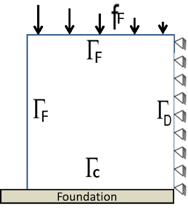
The physical setting of the example is depicted in Figure 1 (left-hand side). The body is in initial contact with a deformable foundation on its lower part while ΓD=ΓA\Gamma_{D}=\Gamma_{A} is the right boundary {1}×[0,1]\{1\}\times[0,1] (and so both the displacement and electric potential fields vanish there). A surface force acts on the upper surface [0,1]×{1}[0,1]\times\{1\} and no electric charges are applied nor in the body or the surface.

Refer to caption
Refer to caption
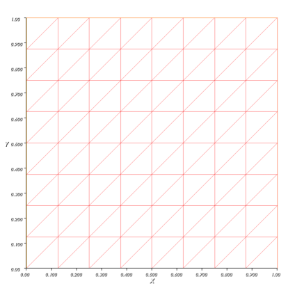
Figure 1: Example 1: Physical setting and mesh example for NelN_{el}=8.
Piezoelectric (C/m2)(C/m^{2}) Permittivity (C2/(Nm2)(C^{2}/(Nm^{2})
e21e_{21} e22e_{22} e13e_{13} β11\beta_{11} β22\beta_{22}
-5.4 15.8 12.3 916 830
Table 1: Material constants.

The numerical solution corresponding to Nel=512N_{el}=512 subdivisions on each outer side of the square (see the right-hand side of Fig. 1 for the case Nel=8N_{el}=8), and k=0.00078612k=0.00078612 has been considered as the “exact” solution in order to compute the numerical errors given by

Ehk=max0nN{𝒖n𝒖nhkV+vnvnhkH+φnφnhkW}.E^{hk}=\displaystyle\max_{0\leq n\leq N}\left\{\|\mbox{\boldmath{$u$}}_{n}-\mbox{\boldmath{$u$}}_{n}^{hk}\|_{V}+\|v_{n}-v_{n}^{hk}\|_{H}+\|\varphi_{n}-\varphi_{n}^{hk}\|_{W}\right\}.

Both the piezoelectric and permittivity coefficients are depicted in Table 1. Moreover the following data have been employed in the simulations:

T=1s,𝒇0(𝒙,t)=𝟎N/m3,𝒇F(𝒙,t)={(0,60(1x1)t)N/m2 if x2=1,𝟎N/m2elsewhere,E=20000N/m2,r=0.3,cp=105,ρ=1kg/m3,φA=0V,q0=0C/m3,qF=0C/m2,𝒖0=𝟎m,𝒗0=𝟎m/s,φ0=0V.\begin{array}[]{l}T=1\,s,\;\;\mbox{\boldmath{$f$}}_{0}(\mbox{\boldmath{$x$}},t)=\mbox{\boldmath{$0$}}\;N/m^{3},\;\;\mbox{\boldmath{$f$}}_{F}(\mbox{\boldmath{$x$}},t)=\left\{\begin{array}[]{l}(0,-60(1-x_{1})t)\;N/m^{2}\;\text{ if $x_{2}$=1,}\\ \mbox{\boldmath{$0$}}\;\>N/m^{2}\quad\text{elsewhere,}\end{array}\right.\\ E=20000\;\;N/m^{2},\quad r=0.3,\quad c_{p}=10^{5},\quad\rho=1\;kg/m^{3},\\ \varphi_{A}=0\;\;V,\quad q_{0}=0\;\;C/m^{3},\quad q_{F}=0\;C/m^{2},\\ \mbox{\boldmath{$u$}}_{0}=\mbox{\boldmath{$0$}}\;\;m,\quad\mbox{\boldmath{$v$}}_{0}=\mbox{\boldmath{$0$}}\;\;m/s,\quad\varphi_{0}=0\;\;V.\end{array}

In Table 2 the numerical errors obtained for some discretization parameters NelN_{el} and kk are shown. As can be seen, the convergence of the numerical algorithm is clearly 
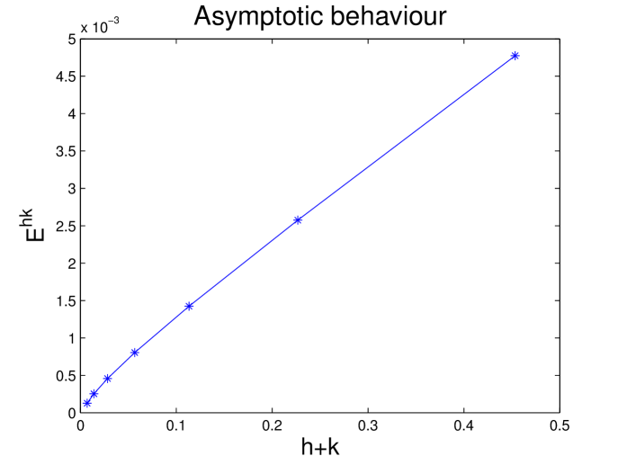
observed. The evolution of the error with respect to the parameter k+hk+h is plotted in Figure 2 (here, h=2Nelh=\frac{\sqrt{2}}{N_{el}}). The linear convergence of the algorithm seems to be achieved.

NelkN_{el}\downarrow k\to 0.0015625 0.003125 0.00625 0.0125 0.025 0.05 0.1
4 0.470744 0.470809 0.470941 0.471220 0.471838 0.473329 0.477455
8 0.255173 0.255208 0.255284 0.255468 0.255957 0.257490 0.263109
16 0.141647 0.141660 0.141698 0.141839 0.142445 0.144762 0.152973
32 0.080098 0.080101 0.080149 0.080420 0.081371 0.084702 0.096829
64 0.045528 0.045547 0.045663 0.046057 0.047449 0.052511 0.069826
128 0.025358 0.025405 0.025569 0.026165 0.028363 0.035951 0.058180
256 0.012722 0.012791 0.013062 0.014099 0.017720 0.028208 0.053679
Table 2: Example 1: Numerical errors (×100\times 100) for some NelN_{el} and kk.
Refer to caption
Figure 2: Example 1: Asymptotic behaviour of the numerical scheme

5.3 A second example: piezoelectric effect

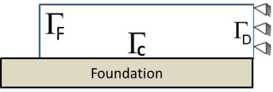
As a second numerical example, in order to observe the effect of the piezoelectric properties of the material, a physical setting as the one depicted in Fig. 3 is considered.

Refer to caption
Figure 3: Example 2: physical setting

In this case the body Ω=[0,4]×[0,1]\Omega=[0,4]\times[0,1] is clamped on its right end and it remains in initial contact with a deformable foundation on its lower boundary. No physical forces act on the body, but a constant surface electric charge (qF=200C/M2q_{F}=200\;C/M^{2}) is applied on the lower part of the boundary, where contact is produced. Here, as in the previous example, we assume that ΓD=ΓA.\Gamma_{D}=\Gamma_{A}.

The following data have been used

T=1s,𝒇B(𝒙,t)=𝟎N/m3,𝒇F=𝟎N/m2,E=2×106N/m2,r=0.3,cp=105,ρ=1000kg/m3,φA=0V,q0=0C/m3,qF={200C/m3 if x2=0,0elsewhere,𝒖0=𝟎m,𝒗0=𝟎m/s,φ0=0V.\begin{array}[]{l}T=1\,s,\quad\mbox{\boldmath{$f$}}_{B}(\mbox{\boldmath{$x$}},t)=\mbox{\boldmath{$0$}}\;\;N/m^{3},\quad\mbox{\boldmath{$f$}}_{F}=\mbox{\boldmath{$0$}}\;\>N/m^{2},\\ E=2\times 10^{6}\;\;N/m^{2},\quad r=0.3,\quad c_{p}=10^{5},\quad\rho=1000\;kg/m^{3},\\ \varphi_{A}=0\;\;V,\quad q_{0}=0\;\;C/m^{3},\quad q_{F}=\left\{\begin{array}[]{l}200\;\;C/m^{3}\text{ if }x_{2}=0,\\ 0\quad\text{elsewhere},\end{array}\right.\\ \mbox{\boldmath{$u$}}_{0}=\mbox{\boldmath{$0$}}\;\;m,\quad\mbox{\boldmath{$v$}}_{0}=\mbox{\boldmath{$0$}}\;\;m/s,\quad\varphi_{0}=0\;\;V.\end{array}
Refer to caption
Figure 4: Example 2: Deformed configuration (x 5000) at final time

We can see in Fig. 4 that deformations appear due to the piezoelectric effect which, added to the mechanical restrictions, lead the body to a stress-state which can be observed in Fig. 5 (right-hand side). In this figure (left-hand side), the electric potential field is shown at final time.

Refer to captionRefer to caption\begin{array}[]{cc}\includegraphics[scale={0.17}]{Test_2_pot}&\includegraphics[scale={0.17}]{Test_2_ten}\end{array}

Figure 5: Example 2: potential field and von mises stress norm at final time.

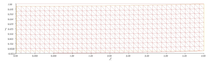
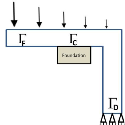
5.4 A third example: deformable contact of an L-shaped domain

As a final example, we consider an L-shaped body which is submitted to the action of traction forces on its upper horizontal boundary. The body is clamped on its lower horizontally boundary and an obstacle is assumed to be in initial contact, as can be observed in Fig. 6.

Refer to caption
Figure 6: Example 3: Contact problem of an L-shaped domain

The following data are used in the simulation:

T=1s,𝒇B(𝒙,t)=𝟎N/m3,𝒇F={(0,500(60x1)t)N/m2 if x2=50,𝟎N/m2elsewhere,E=2.1×109N/m2,r=0.3,cp=105,ρ=27000kg/m3,φA=0V,q0=0C/m3,qF=0C/m3,𝒖0=𝟎m,𝒗0=𝟎m/s,φ0=0V.\begin{array}[]{l}T=1\,s,\quad\mbox{\boldmath{$f$}}_{B}(\mbox{\boldmath{$x$}},t)=\mbox{\boldmath{$0$}}\;\;N/m^{3},\quad\mbox{\boldmath{$f$}}_{F}=\left\{\begin{array}[]{l}(0,-500(60-x_{1})t)\;N/m^{2}\;\text{ if $x_{2}$=50,}\\ \mbox{\boldmath{$0$}}\;\>N/m^{2}\quad\text{elsewhere,}\end{array}\right.\\ E=2.1\times 10^{9}\;\;N/m^{2},\quad r=0.3,\quad c_{p}=10^{5},\quad\rho=27000\;kg/m^{3},\\ \varphi_{A}=0\;\;V,\quad q_{0}=0\;\;C/m^{3},\quad q_{F}=0\;\;C/m^{3},\\ \mbox{\boldmath{$u$}}_{0}=\mbox{\boldmath{$0$}}\;\;m,\quad\mbox{\boldmath{$v$}}_{0}=\mbox{\boldmath{$0$}}\;\;m/s,\quad\varphi_{0}=0\;\;V.\end{array}

Both electric potential and von Mises stress norm are plotted, over the final configuration of the body and at final time, in Fig. 7. The area of maximum stress concentration is located near the contact boundary due to the bending movement, and it coincides with the region where the electric potential reaches its maximum value as it was expected.

Refer to captionRefer to caption\begin{array}[]{cc}\includegraphics[scale={0.4}]{Test_3_pot}&\includegraphics[scale={0.4}]{Test_3_mises}\end{array}

Figure 7: Example 3: potential field and von mises stress norm over the deformed mesh (×500\times 500) at final time.

Acknowledgements

The work of M. Campo and J.R. Fernández was supported by the Ministerio de Economía y Competitividad under the research project MTM2012-36452-C02-02 (with the participation of FEDER) and the work of Á. Rodríguez-Arós and J.M. Rodríguez was supported by the research project MTM2012-36452-C02-01 with the participation of FEDER.

References

  • [1] J. Ahn, Thick obstacle problems with dynamic adhesive contact, M2AN Math. Model. Numer. Anal. 42(6) (2008) 1021-1045.
  • [2] J. Ahn and D.E. Stewart, Dynamic frictionless contact in linear viscoelasticity, IMA J. Numer. Anal. 29(1) (2009) 43–71.
  • [3] M. Attia, A. El-Shafei and F. Mahmoud, Analysis of nonlinear thermo-viscoelastic-viscoplastic contacts, Internat. J. Engrg. Sci. 78 (2014) 1-17.
  • [4] M. Barboteu, K. Bartosz, W. Han, and T. Janiczko, Numerical analysis of a hyperbolic hemivariational inequality arising in dynamic contact, SIAM J. Numer. Anal. 53(1) (2015) 527–550.
  • [5] M. Barboteu, J.R. Fernández and T.-V. Hoarau-Mantel, A class of evolutionary variational inequalities with applications in viscoelasticity, Math. Models Methods Appl. Sci. 15(10) (2005) 1595-1617.
  • [6] M. Barboteu, J.R. Fernández and Y. Ouafik, Numerical analysis of a frictionless viscoelastic piezoelectric contact problem, M2AN Math. Model. Numer. Anal. 42(4) (2008) 667-682.
  • [7] M. Barboteu, J.R. Fernández and R. Tarraf, Numerical analysis of a dynamic piezoelectric contact problem arising in viscoelasticity, Comput. Methods Appl. Mech. Engrg. 197(45-48) (2008) 3724-3732.
  • [8] M. Barboteu and M. Sofonea, Modeling and analysis of the unilateral contact of a piezoelectric body with a conductive support, J. Math. Anal. Appl. 358(1) (2009) 110-124.
  • [9] V. Barbu, Nonlinear Semigroups and Differential Equations in Banach Spaces, Editura Academiei, Bucharest-Noordhoff, Leyden, 1976.
  • [10] P. Barral, M.C. Naya-Riveiro and P. Quintela, Mathematical analysis of a viscoelastic problem with temperature-dependent coefficients. I. Existence and uniqueness. Math. Methods Appl. Sci. 30(13) (2007) 1545-1568.
  • [11] R.C. Batra and J.S. Yang, Saint-Venant’s principle in linear piezoelectricity, J. Elasticity 38 (1995) 209–218.
  • [12] A. Berti and M.G. Naso, Unilateral dynamic contact of two viscoelastic beams, Quart. Appl. Math. 69(3) (2011) 477-507.
  • [13] M. Campo, J.R. Fernández, W. Han and M. Sofonea, A dynamic viscoelastic contact problem with normal compliance and damage, Finite Elem. Anal. Des. 42(1) (2005) 1-24.
  • [14] M. Campo, J.R. Fernández, K.L. Kuttler, M Shillor and J.M. Viaño, Numerical analysis and simulations of a dynamic frictionless contact problem with damage, Comput. Methods Appl. Mech. Engrg. 196 476-488 (2006).
  • [15] T.A. Carniel, P.A. Muñoz-Rojas and M. Vaz, A viscoelastic viscoplastic constitutive model including mechanical degradation: uniaxial transient finite element formulation at finite strains and application to space truss structures, Appl. Math. Model. 39(5-6) (2015) 1725-1739.
  • [16] H. Chen, W. Xu, W. Wang, R. Wang, C. Shi, A nonlinear viscoelastic-plastic rheological model for rocks based on fractional derivative theory, Internat. J. Modern Phys. B 27(25) (2013) 1350149.
  • [17] P.G. Ciarlet, Basic error estimates for elliptic problems. In: Handbook of Numerical Analysis, P.G. Ciarlet and J.L. Lions eds., vol II (1993), pp. 17-351.
  • [18] M. Cocou, Existence of solutions of a dynamic Signorini’s problem with nonlocal friction in viscoelasticity, Z. Angew. Math. Phys. 53(6) (2002) 1099-1109.
  • [19] M. Cocou and G. Scarella, Analysis of a dynamic unilateral contact problem for a cracked viscoelastic body, Z. Angew. Math. Phys. 57(3) (2006) 523-546.
  • [20] M. Cocu and J.M. Ricaud, Analysis of a class of implicit evolution inequalities associated to dynamic contact problems with friction, Internat. J. Eng. Sci. 328 (2000) 1534-1549.
  • [21] M.I.M. Copetti and J.R. Fernández, A dynamic contact problem involving a Timoshenko beam model, Appl. Numer. Math. 63 (2013) 117-128.
  • [22] Y. Dumont and L. Paoli, Dynamic contact of a beam against rigid obstacles: convergence of a velocity-based approximation and numerical results, Nonlinear Anal. Real World Appl. 22 (2015) 520-536.
  • [23] G. Duvaut and J.L. Lions, Inequalities in mechanics and physics, Springer Verlag, Berlin, 1976.
  • [24] C. Eck, J. Jarusek and M. Krbec, Unilateral contact problems. Variational methods and existence theorems, Pure and Applied Mathematics, 270, Chapman & Hall/CRC, Boca Raton, 2005.
  • [25] M. Fabrizio and S. Chirita, Some qualitative results on the dynamic viscoelasticity of the Reissner-Mindlin plate model, Quart. J. Mech. Appl. Math. 57(1) (2004) 59-78.
  • [26] J.R. Fernández and D. Santamarina, An a posteriori error analysis for dynamic viscoelastic problems, M2AN Math. Model. Numer. Anal. 45 (2011) 925-945.
  • [27] H. Ghoneim and Y. Chen, A viscoelastic-viscoplastic constitutive equation and its finite element implementation, Computers Struct. 17(4) (1983) 499-509.
  • [28] F. Hecht, New development in FreeFem++, J. Numer. Math. 20(3-4) (2012) 251-265.
  • [29] D.W. Holmes and J.G. Loughran, Numerical aspects associated with the implementation of a finite strain, elasto-viscoelastic-viscoplastic constitutive theory in principal stretches, Internat. J. Numer. Methods Engrg. 83(3) (2010) 366-402.
  • [30] T. Ideka, Fundamentals of piezoelectricity, Oxford University Press, Oxford, 1990.
  • [31] I.R. Ionescu and Q.-L. Nguyen, Dynamic contact problems with slip dependent friction in viscoelasticity, Internat. J. Appl. Math. Comput. Sci. 12 (2002) 71-80.
  • [32] J. Jaruśek and C. Eck, Dynamic contact problems with small Coulomb friction for viscoelastic bodies. Existence of solutions. Math. Models Methods Appl. Sci. 9(1) (1999) 11-34.
  • [33] J.S. Kim and A.H. Muliana, A time-integration method for the viscoelastic-viscoplastic analyses of polymers and finite element implementation, Internat. J. Numer. Methods Engrg. 79(5) (2009) 550-575.
  • [34] A. Klarbring, A. Mikelić and M. Shillor, Frictional contact problems with normal compliance, Internat. J. Engrg. Sci. 26 (1988) 811-832.
  • [35] K.L. Kuttler, Dynamic friction contact problem with general normal and friction laws, Nonlinear Anal. 28 (1997) 559-575.
  • [36] K.L. Kuttler and M. Shillor, Dynamic bilateral contact with discontinuous friction coefficient, Nonlinear Anal. 45 (2001) 309-327.
  • [37] Y. Li and Z. Liu, Dynamic contact problem for viscoelastic piezoelectric materials with slip dependent friction. Nonlinear Anal. 71(5-6) (2009) 1414-1424.
  • [38] X. Li and M. Wang, Hertzian contact of anisotropic piezoelectric bodies, J. Elasticity 84(2) (2006) 153-166.
  • [39] F. Mahmoud, A. El-Shafei and M. Attia, Modeling of nonlinear viscoelastic-viscoplastic frictional contact problems, Internat. J. Engrg. Sci. 74 (2014) 103-117.
  • [40] J.A.C. Martins and J.T. Oden, Existence and uniqueness results for dynamic contact problems with nonlinear normal and friction interface laws, Nonlinear Anal. 11 (1987) 407-428.
  • [41] B. Miled, I. Doghri and L. Delannay, Coupled viscoelastic-viscoplastic modeling of homogeneous and isotropic polymers: numerical algorithm and analytical solutions, Comput. Methods Appl. Mech. Engrg. 200(47-48) (2011) 3381-3394.
  • [42] R.D. Mindlin, Polarisation gradient in elastic dielectrics, Internat. J. Solids Structures 4 (1968) 637-663.
  • [43] R.D. Mindlin, Continuum and lattice theories of influence of electromechanical coupling on capacitance of thin dielectric films, Internat. J. Solids Structures 4 (1969) 1197-1213.
  • [44] S. Migórski, A. Ochal and M. Sofonea, Analysis of a dynamic contact problem for electro-viscoelastic cylinders, Nonlinear Anal. 73(5) (2010) 1221-1238.
  • [45] A. Morro and B. Straughan, A uniqueness theorem in the dynamical theory of piezoelectricity, Math. Methods Appl. Sci. 14(5) (1991) 295-299.
  • [46] M. Sofonea, W. Han and M. Shillor, Analysis and Approximation of Contact Problems with Adhesion or Damage, Pure and Applied Mathematics, 276, Chapman & Hall/CRC, Boca Raton, 2006.
  • [47] R.A. Toupin, Stress tensors in elastic dielectrics, Arch. Ration. Mech. Anal. 5 (1960) 440-452.
  • [48] R.A. Toupin, A dynamical theory of elastic dielectrics, Internat. J. Engrg. Sci. 1 (1963) 101-126.