Analysis of power system inertia estimation in high wind power plant integration scenarios
Abstract
Nowadays, power system inertia is changing as a consequence of replacing conventional units by renewable energy sources, mainly wind and PV power plants. This fact affects significantly the grid frequency response under power imbalances. As a result, new frequency control strategies for renewable plants are being developed to emulate the behaviour of conventional power plants under such contingencies. These approaches are usually called ’virtual inertia emulation techniques’. In this paper, an analysis of power system inertia estimation from frequency excursions is carried out by considering different inertia estimation methodologies, discussing the applicability and coherence of these methodologies under the new supply-side circumstances. The modelled power system involves conventional units and wind power plants, including wind frequency control strategies in line with current mix generation scenarios. Results show that all methodologies considered provide an accurate result to estimate the equivalent inertia based on rotational generation units directly connected to the grid. However, significant discrepancies are found when frequency control strategies are included in wind power plants decoupled from the grid. In this way, authors consider that it is necessary to define alternative inertia estimation methodologies by including virtual inertia emulation. Extensive discussion and results are also provided in this study.
1 Introduction
Frequency of a power system deviates from its nominal value after a severe power imbalance between generation and consumption babahajiani18 . Due to the increasing penetration of renewable energy sources (RES), mainly wind and PV, electrical grids can suffer more frequency stability challenges cvetkovic17 . RES are intermittent and uncertain because they depend on weather conditions wang15 . This fact makes them hard to integrate into power systems teng17 , as they pose stress on their operation rodriguez14 : Transmission System Operators (TSOs) have to deal with not only the uncontrollable demand but also uncontrollable generation zhang17 .
Moreover, renewable power plants are not connected to the grid through synchronous machines, but through electronic converters junyent15 . Thus, by increasing the amount of renewable sources and replacing synchronous conventional units, the effective rotational inertia of the system can be significantly reduced akhtar15 ; yang18 . The rotational inertia is important to limit the rate of change of frequency (ROCOF) right after a power imbalance dehghanpour15 . Therefore, power systems with lower equivalent inertia are initially more sensitive to frequency deviations kim16 ; nguyen18 . As a result, frequency control strategies have been developed to effectively integrate RES into the grid gross17increasing . Such methods are commonly referred to as synthetic, artificial, emulated or virtual inertia vokony17 .
The aim of this paper is to estimate and compare the equivalent inertia constant of a power system with high RES integration from the frequency deviations suffered after an imbalance. Several methodologies have been proposed during the last decades in the specific literature inoue97 ; chassin05 ; wall12 ; wall14 ; zografos17 ; tuttelberg18 ; zografos18 . The power system considered in this paper is in line with current grids, involving conventional and wind power plants. Moreover, wind plants include frequency control according to a recent approach fernandez18 . The rest of the paper is organized as follows: the theoretical background of the problem is covered in Section 2. Section 3 reviews and explains the different strategies to estimate the inertia constant of a power system after an imbalance. In Section 4, the power system and different scenarios considered in this paper are detailed. Results are discussed in Section 5. Conclusions are given in Section 6.
2 Theoretical background
2.1 Inertia constant
From a traditional point of view, after a power imbalance, the kinetic energy stored in the rotating masses of a generator is released following expression (1) ulbig14 :
| (1) |
where is the moment of inertia and is the rated rotational frequency of the machine. The inertia constant of a generator is defined as the ratio between the stored kinetic energy and its rated power uriarte15 . determines the time interval during which an electrical generator can supply its rated power only by using the kinetic energy stored in its rotating masses tielens16 :
| (2) |
Depending on the type of conventional units (i.e., steam, combined cycle, hydroelectric, etc.), typical inertia constants are in the range of 2–10 s, as indicated in Table 2.1.
according to generation type, rated power and reference \topruleType of power plant Rated power (MW) (s) Ref. Year \midruleThermal (2 poles) Not indicated 2.5-6 kundur94 1994 Thermal (4 poles) Not indicated 4-10 kundur94 1994 Thermal 10 4 de07 2007 Thermal 500-1500 2.3-2 anderson08 2008 Thermal 1000 4-5 dabur11 2011 Thermal Not indicated 4-5 kumal12 2012 Thermal (steam) 130 4 tielens12 2012 Thermal (steam) 60 3.3 tielens12 2012 Thermal (combined cycle) 115 4.3 tielens12 2012 Thermal (gas) 90-120 5 tielens12 2012 Thermal (nuclear) 100-1400 4 tielens16 2016 Thermal (fossil) 0-1000 5-3 tielens16 2016 \midruleHydroelectric Not indicated 2-4 kundur94 1994 Hydroelectric 200 rpm Not indicated 2-3 grainger94 1994 Hydroelectric 200 rpm Not indicated 2-4 grainger94 1994 Hydroelectric 450<n<514 rpm 10-65 2-4.3 anderson08 2008 Hydroelectric 200<n<400 rpm 10-75 2-4 anderson08 2008 Hydroelectric 138<n<180 rpm 10-90 2-3.3 anderson08 2008 Hydroelectric 80<n<120 rpm 10-85 1.75-3 anderson08 2008 Hydroelectric Not indicated 4.75 eremia13 2013 \botrule
2.2 Swing equation of a power system. Equivalent rotational system inertia
Power systems include several synchronous generators. Thus, it is possible to estimate the equivalent rotational system inertia () by using spahic16 :
| (3) |
refers to the inertia constant of power plant , is the rated power of power plant , is the rated power of the power system and is the total number of conventional plants.
The swing equation of a power system is used to analyse transient stability problems, as well as frequency control design and regulation raisz18 . Moreover, it relates frequency excursions with the power imbalance tofis17 :
| (4) |
where is the deviation of the grid frequency, is the equivalent inertia constant for the power system determined by (3), is the mechanical power change supplied by generator and is the electrical power demand variation.
Some electrical loads are frequency dependent (such as rotating machines). Consequently, is expressed as suh17 :
| (5) |
being the power change of frequency independent loads and the damping factor (load-frequency response constant). Combining (4) and (5), the swing equation of a power system is obtained yazdi19 .
| (6) |
2.3 Future definition of inertia constant of a power system
By considering policies to promote the integration of renewables, RES have replaced conventional power plants and, subsequently, synchronous generators li17design . Among the different renewable sources available, PV and wind (especially doubly fed induction generators, DFIG ochoa17 ) are the two most promising resources for generating electrical energy shah15 . Both wind and PV power plants are controlled by power converters according to the maximum power point tracking (MPPT) control muyeen10 ; mohamed12 . This technique prevents both sources to directly contribute to the inertia of the system zhao16 ; hosseinipour17 ; tielens17phd , which is considered as one of the main drawbacks to integrate large amounts of RES into the grid du18 . In fact, modern wind turbines have rotational inertia constants comparable to those of conventional generators, provided by their blades, drive train and electrical generator. However, this inertia is hidden from the power system point of view due to the converter yingcheng11 . Moreover, ROCOF depends on the available inertia ulbig15 . As a result, larger frequency deviations are achieved after an imbalance between supply-side and demand when RES replace conventional units without providing frequency response nedd17 .
Therefore, it is necessary that RES become an active agent in grid frequency regulation you17 . Actually, several TSOs are requiring that RES contribute to ancillary services as well aho12 , especially wind power plants kayikcci09 . Toulabi et al. affirm that the participation of wind turbines in frequency control is necessary toulabi17 . Under these requirements, different solutions providing inertia and frequency control from RES have been under study during the last decades. These technologies are usually known as ‘virtual inertia techniques’ tamrakar17 and are explained in sun10 ; tamrakar17 ; attya18 ; wang18 ; ziping18 .
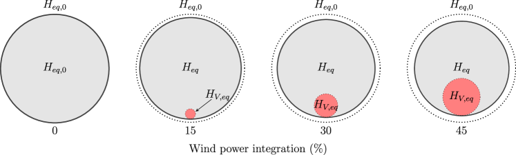
If RES providing frequency response were considered, the equivalent inertia of the power system would have two different components: synchronous rotational inertia due to conventional generators , calculated with eq. (3), and virtual inertia corresponding to RES, , as indicated in eq. (7) morren06phd ; tielens17 . In this way, refers to the emulated inertia constant of power plant , is the rated power of power plant and is the total number of virtual generators included in the power system under consideration. The rest of the parameters are the same as (3).
| (7) |
However, the values of are not normally known and can be time dependent. Thus, it is difficult to apply eq. (7).
3 Inertia estimation strategies. Methodology
Different inertia estimation strategies have been proposed during the last decades inoue97 ; chassin05 ; wall12 ; wall14 ; zografos17 ; tuttelberg18 ; zografos18 . Damping factor is neglected in most approaches as its effects are small on the firsts moments of the imbalance .
Inoue et al. propose a procedure for estimating the inertia constant of a power system using transients of the frequency measured at an imbalance inoue97 . At the onset of an imbalance , the frequency deviation is . Assuming that the imbalance is known, and by estimating the ROCOF () at , the inertia constant can be calculated with
| (8) |
To calculate the ROCOF, a degree polynomial approximation of with respect to time is fitted. The time interval is about 15 to 20 s after the imbalance
| (9) |
where is the time. By estimating the coefficients to , the equivalent inertia constant is obtained by using eq. (11), as is approximately equal to the ROCOF at
| (10) |
| (11) |
Chassin et al chassin05 frequency and power values from the Western Electricity Coordination Council were collected. In this case, ROCOF is estimated by removing noise from the frequency data recorded and applying the first derivative. The equation to estimate is as below
| (12) |
Wall et al. present a robust estimation method for the inertia available in the system wall12 ; wall14 . It uses as input data the active power and the derivative of frequency , measured from a single location. The proposed algorithm consists of a set of four filters (two for the total active power – and – and two for the ROCOF – and –) applied as sliding windows, see Figure 1. Windows have a width of data points and they are separated by a width .
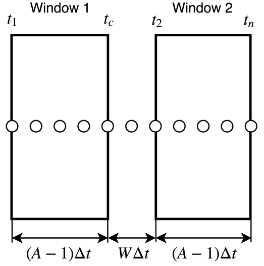
is estimated by the following expression:
| (13) |
where , , and are calculated with (14):
| (14) | ||||
The result of applying eq. (13) is only during the time in which the power imbalance has occurred () wall14 .
Zografos and Ghandhari zografos17 consider an aggregated load model to represent the behaviour of the average system load. The load power change is expressed by
| (15) |
where is the total power production before the disturbance and is the system’s overall voltage profile, approximated by the voltage of the generator buses according to
| (16) |
being the voltage at the bus of generator at time , the voltage before the disturbance at the bus of generator and the number of connected generators. By combining (6) and (15), the inertia constant of the system is calculated from (17), where is the size of the disturbance at the moment of the disturbance
| (17) |
Tuttelberg et al. tuttelberg18 simplify the dynamic response to a reduced order system with the generic form of (18)
| (18) |
The inertia of a power system can be determined by the value of its unit impulse response at . For a transfer function like the one presented in (18), the first value of the impulse response can be evaluated in Matlab with: the impulse function, the gain value of the zero-pole model from tf2zpk or as the ratio of to .
Zografos et al. zografos18 introduce two approaches to express the power change due to the frequency and voltage dynamics ( and approaches, respectively)
| (19) |
where is the size of the disturbance, and and deal with the power change due to the frequency and the voltage dynamics, respectively.
In the approach, it is considered that . To obtain , the governor’s behavior is analysed. relates the mechanical power change and the frequency deviation. It is considered that
| (20) |
being the mechanical power change and an unknown time varying function that accommodates the dynamic response of the system related to . Then eq. (6) is converted into
| (21) |
where is the estimated inertia constant to be found. However, as previously said, is also unknown. To compute , a specific selected time is considered. is recommended to be the first local extreme of the ROCOF curve after the moment of the disturbance. Moreover, eq. (21) is considered for discrete points equally distributed around . can thus be approximated by the average of the values of of the neighbouring points to . Therefore, a system with linear equations and unknowns is obtained (25). By solving it, is obtained
| (25) |
In the approach, it is considered that . To obtain , the load power change due to voltage dependency is analysed
| (26) |
where is the total power production before the disturbance, , and define the fraction of each component, and is the loads’ aggregated voltage profile, calculated with (16). Then
| (27) |
The application range of this strategy should be selected before 500 ms, and as soon as possible after the disturbance to avoid the governor frequency response.
The estimated equivalent inertia is calculated with (28), where is recommended to be the estimated with (25)
| (28) |
Finally, Table 3 summarizes the different inertia estimation methodologies discussed in this work. As can be seen, most of them are based on the power imbalance and ROCOF, in line with the swing equation and the frequency control of conventional generation units.
Summary of inertia estimation methodologies \topruleRef. Methodology based on Year \midruleinoue97 Power imbalance and ROCOF 1997 chassin05 Power imbalance and ROCOF 2005 wall12 Total power supplied and ROCOF 2012 wall14 Total power supplied and ROCOF 2014 zografos17 Power imbalance and ROCOF 2017 tuttelberg18 Impulse function 2018 zografos18 Power imbalance and ROCOF 2018 \botrule
4 System identification
4.1 Power system modelling
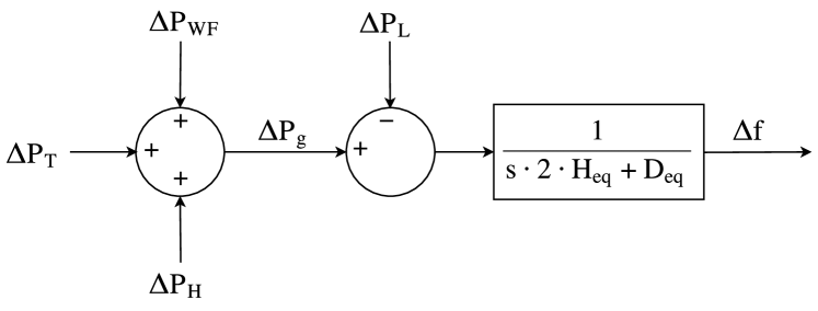
From the supply-side, the power system considered for simulation purposes involve conventional generating units (thermal and hydro-power plants) and wind power plants. A simplified diagram of the power system can be seen in Figure 2, being the variation of the generated power , and the power imbalance. A base power of 1350 MW is assumed, corresponding to the capacity of the power system. It is considered that the active power of loads is independent on voltage, and as a consequence, the term of eq. (17) zografos17 is not considered, and the approach of Zografos et al. zografos18 is not taken into account. The equivalent damping factor of loads is puMW/puHz kundur94 . Simulations have been carried out in Matlab/Simulink.
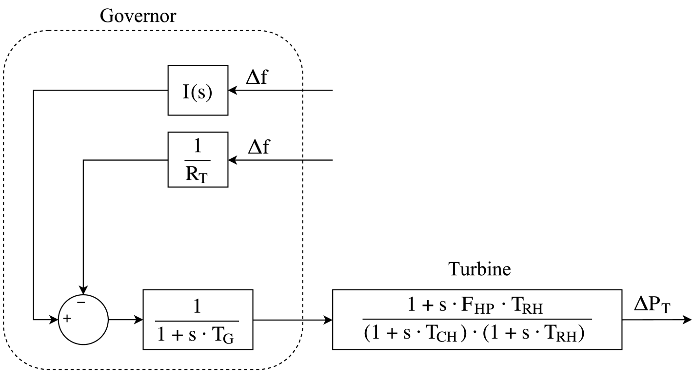
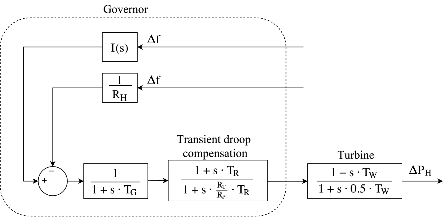
Conventional units are modelled according to the simplified governor-based models widely used and proposed in kundur94 , see Figure 3. The inertia constant for these power plants are s and s. Wind power plants are modelled according to an equivalent wind turbine, with the mechanical single-mass and turbine control models presented in miller03 ; ullah08 ; clark10 . The frequency controller is included in the wind turbine model as can be seen in Figure 4. Parameters of both conventional and wind power plants are summarized in the Appendix.
(a)Reheat thermal power plant \figfooter(b)Hydro-power

4.2 Frequency control strategies
Under power imbalance conditions, the governor control mechanisms of conventional units modify their active power supply to recover system power balance and, thus, remove the frequency deviation diaz14 . Grid frequency deviation is subsequently used as an input signal for primary and secondary frequency controls alomoush10 . Primary frequency control is performed locally at the generator, being the active power increment/decrement proportional to through the speed regulation parameter dai12 . Secondary frequency control involves an integral controller that modifies the turbine set-point of each generation unit simpson15 .
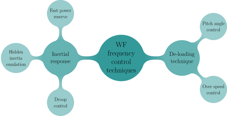
Wind turbines can also include frequency control strategies. Different solutions have been proposed in the last decade. These strategies are usually classified as indicated in Figure 5 dreidy17 , excluding the use of energy storage systems. According to the specific literature, examples of these strategies are summarized in Table 4.2.
Moreover, some approaches can be combined, in order to improve the frequency deviation after the power imbalance margaris12 ; zhang12 ; ye15 ; abo16 ; hwang16 ; van16 ; liu19 . As can be seen, an alternative classification can be then proposed: not-including derivative frequency dependence and including derivative frequency dependence. An additional active power is added to the pre-event power supplied by the wind power plant in all the cases except de-loading technique. In the fast power reserve, can be defined: as a constant, proportional to the rotational speed of the turbine or proportional to the frequency excursion, depending on the reference. The hidden inertia emulation uses a proportional derivative controller, being and the derivative and proportional constants of the controller, respectively. With regard to the droop control, is proportional to the frequency deviation by the droop constant . As discussed in Section 5, this frequency controllers modify considerably the estimated inertia values and addresses significant discrepancies among methodologies.
Wind turbines frequency control proposals \topruleRef. Type of control Definition Year \midruletarnowski09 Fast power reserve , 2009 keung09 Fast power reserve , 2009 chang11 Fast power reserve , 2011 itani11 Fast power reserve , 2011 hansen14 Fast power reserve , 2014 kang15 Fast power reserve , 2015 hafiz15 Fast power reserve , 2015 kang16 Fast power reserve , 2016 fernandez18 Fast power reserve , 2018 \midrulesu12 Hidden inertia emulation 2012 zhang12 Hidden inertia emulation 2012 zhang13 Hidden inertia emulation 2013 you15 Hidden inertia emulation 2015 hwang16 Hidden inertia emulation 2016 \midrulebonfiglio16 Droop 2016 persson16 Droop 2016 ye17 Droop 2017 jahan19 Droop 2019 \midrulewilches16 Pitch angle deloading — 2016 \botrule
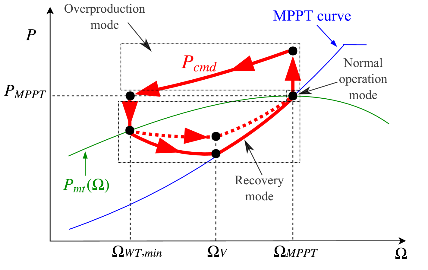
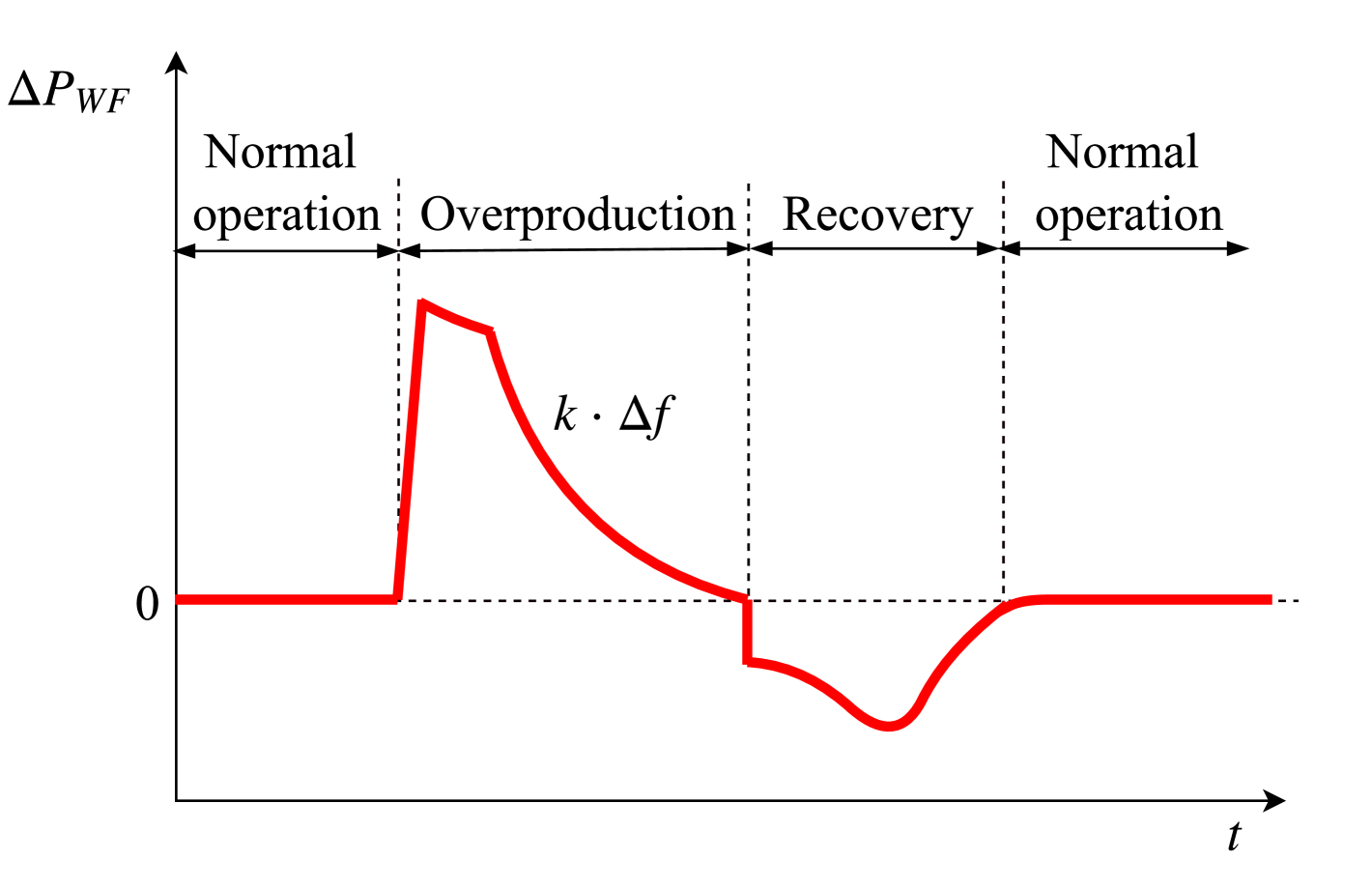
The strategy for VSWTs implemented in this paper is based on the fast power reserve technique presented in fernandez18 for for isolated power systems and assessed in fernandez18fast for multi-area power systems. As indicated in Figure 6, under power imbalance conditions three operation modes are considered: normal operation mode, overproduction mode and recovery mode. Different commanded active power () values are determined aiming to restore the grid frequency. Figure 6a depicts the trajectory of in a plot, indicating the three different operation modes. In Figure 6b, the VSWTs active power variations () submitted to an under-frequency excursion can be seen, being .
(a)Frequency control strategy \figfooter(b) with frequency control strategy
-
i.
In the normal operation mode, the VSWTs operate at the maximum available active power for the current wind speed and the available mechanical power ().
(29) When a generation-load mismatch occurs, the frequency controller strategy switches to the overproduction mode,
(30) -
ii.
In the overproduction mode, the active power supplied by the VSWTs () is over the available mechanical power curve. The additional active power is provided by the kinetic energy stored in the rotational masses, and is proportional to to emulate primary frequency control of conventional generation units margaris12 .
(31) Overproduction mode remains active until: either the rotational speed reaches a minimum allowed value or the commanded power is lower than the maximum available active power ,
(34) -
iii.
In the recovery mode, the power supplied by the VSWTs () is based on two periods: following a parabolic trajectory until the middle of the rotational speed deviation ( in Figure 6a) and through an estimated curve proportional to the difference between and , being the proportionality constant.
(37) The normal operation mode is recovered when either or are reached by the VSWTs.
(40)
4.3 Scenarios
Four different scenarios have been considered for simulations. The first scenario includes only conventional generation units: 88% comes from thermal power plants and 12% from hydro-power plants. Hydro-power capacity remains constant in all the scenarios (12%). However, thermal and wind capacities change depending on the scenario to be simulated by giving a power system with high integration of RES, see Table 4.3. The equivalent inertia constant determined by (3) is also indicated in Table 4.3. The power imbalance considered is pu in all simulations.
Capacity of generating units \topruleSource Scenario 1 Scenario 2 Scenario 3 Scenario 4 \midruleThermal 88% 73% 58% 43% Hydro-power 12% 12% 12% 12% Wind 0% 15% 30% 45% based on (3) 4.80 s 4.05 s 3.30 s 2.55 s \botrule
5 Results
According to the different methodologies discussed in Section 3, the equivalent inertia constant is estimated from the frequency deviations after a power imbalance. Two different approaches are considered and compared in this work:
-
i.
Wind power plants without participation in frequency control.
-
ii.
Wind power plants with participation in frequency control.
(a)Estimated when wind power plants do not participate in frequency control \figfooter(b)Estimated when wind power plants participate in frequency control
Figure 7a depicts the estimated according to the different methodologies without considering wind power plant participation in frequency control. In this case, . The different approaches of inertia estimation provide an accurate approximation of the directly connected rotational inertia calculated with eq. (3). The deviation from the estimated inertia value is lower that a 10% error.
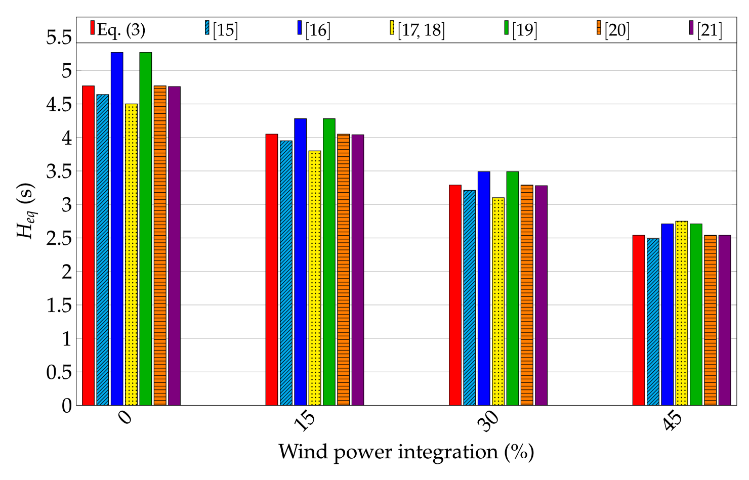
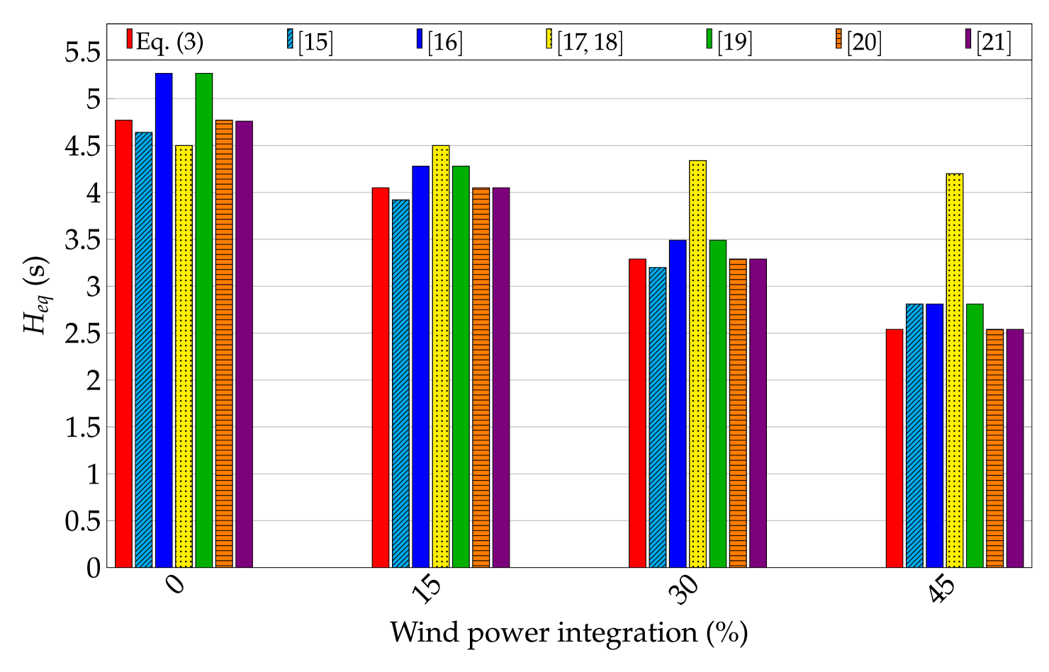
In addition, Figure 7b summarizes the estimated from the different methodologies when wind power plants participate in frequency control. In this case, it is expected that the estimated values from include the virtual inertia referred to eq. (7). However, as can be seen, most methodologies only provide the rotational inertia directly connected to the grid inoue97 ; chassin05 ; zografos17 ; tuttelberg18 ; zografos18 , neglecting the ’virtual inertia’ emulated and provided by the wind power plants. With these methodologies, the estimation of is again accurate to the value calculated by eq. (3), having a deviation lower that a 10% error.
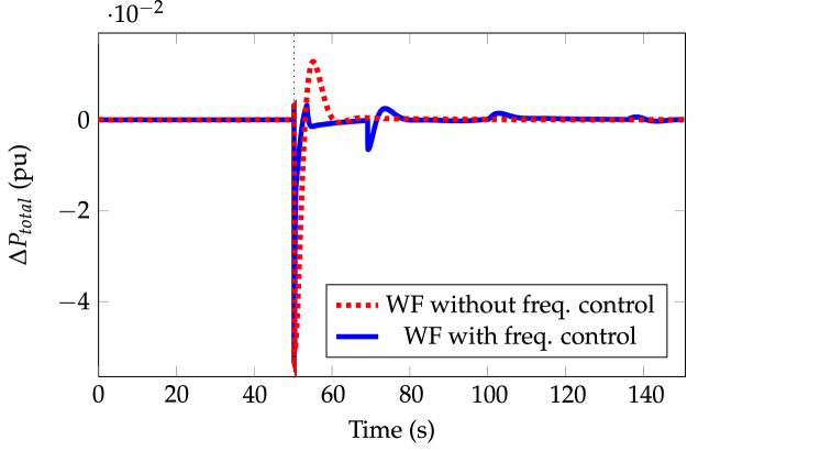
The frequency controller applied on the equivalent wind turbine doesn’t include a derivative dependence control, see Section 4.2. As a consequence, the ROCOF is hardly modified in comparison to scenarios where wind power plants are excluded from the frequency control. At the beginning of the frequency oscillations, values don’t change significantly —see Fig. 8b—, regardless of the integration and participation of wind power plants into the frequency control. Table 5 summarizes these ROCOF values () depending on the participation of wind power plants into frequency control.
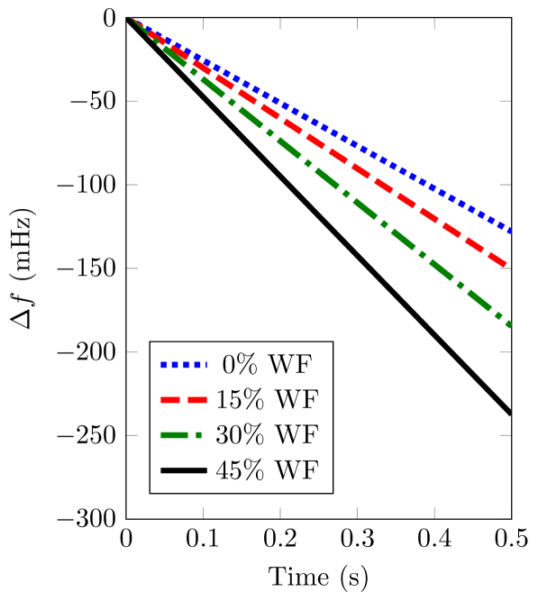
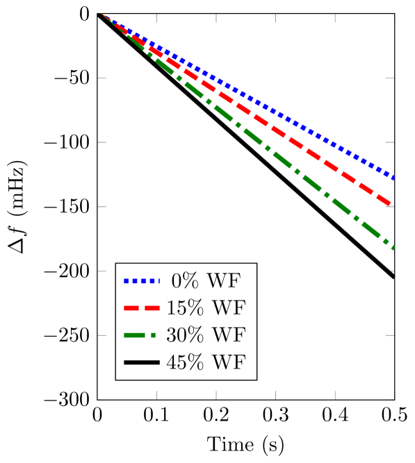
(a)Wind power plants do not participate in frequency control \figfooter(b)Wind power plants participate in frequency control
ROCOF values () depending on the participation of wind power plants into frequency control \toprule Wind power integration 0% 15% 30% 45% \midruleWithout control -256.06 -301.08 -369.20 -474.70 With control -256.06 -298.45 -364.90 -410.10 \botrule
Methodologies inoue97 ; chassin05 ; zografos17 ; zografos18 estimate based on the power imbalance and the ROCOF. is the same in all the scenarios ( pu), and the ROCOF values are similar regardless of the participation of wind power plants into frequency control as aforementioned. As a result, the estimated barely changes despite of including wind power plants into frequency control. Tuttelberg et al. apply an impulse function to the dynamic response, estimating by its value at tuttelberg18 . Only wall12 ; wall14 , by considering the total active power supplied and the ROCOF —referred to eq. (13)—, estimates the equivalent inertia as a combination of rotational and virtual inertias as were expressed in (7).
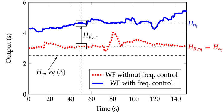
Figure 9 compares the equivalent inertia with and without frequency control from wind power plants in Scenario 4. This inertia is estimated according to wall12 ; wall14 . Total power variation and ROCOF are also depicted for the sake of clarity. The disturbance time is s. As indicated in wall12 ; wall14 (and previously mentioned in Section 3), Figure 9a is only the equivalent inertia around , as squared in the figure. Moreover, when wind power plants don’t participate in frequency control, the equivalent inertia obtained is similar to the value calculated with eq. (3), as already mentioned in Figure 7a. However, a significant difference exists in the estimated equivalent inertia when wind power plants include frequency control. This increasing is due to the ’virtual inertia’ provided by the wind frequency control. This virtual inertia thus depends on how relevant is the wind integration into the generation mix. Moreover, a linear relationship has been found between the wind power integration and the virtual inertia with . The linear relationship can be determined as
| (41) |
being the wind power integration into the grid (in %). Considering eq. (7), (41) and the base power MW, it is obtained that the virtual inertia constant coming from wind turbines is s, in line with the typical rotational inertia constants of conventional plants (refer to Section 2.1) and the wind turbines inertia values proposed by some authors during the last decade tielens12 ; yang12 ; arani13 ; tielens16 .
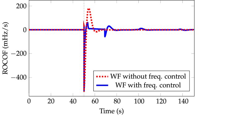
(a)Estimated equivalent inertia (s) \figfooter(b)Total power variation (pu) \figfooter(c)ROCOF (mHz/s)

(a) according to inoue97 ; chassin05 ; zografos17 ; tuttelberg18 ; zografos18 \figfooter(b) according to wall12 ; wall14
Finally, Figure 10b summarizes the simulated scenarios in terms of the estimated from the different methodologies when frequency control is also provided by wind power plants. As can be seen, and depending on the methodology, these approaches address significant discrepancies on the equivalent inertia values. Actually, some of them include some virtual inertia from the wind turbine frequency control of fernandez18 , whereas the others consider their effects barely significant regarding to the equivalent system inertia. Therefore, both wind power plant frequency control strategies and equivalent inertia estimation methodologies must be revised in detail to give suitable results and avoid significant discrepancies among the different proposals in the new mix generation scenarios.
6 Conclusion
In this paper, an analysis and comparison of power system inertia estimation methodologies has been carried out. Different approaches proposed in the literature have been implemented and tested under four different supply-side scenarios including thermal, hydro-power and wind power plants from the supply-side, according to current mix generation road-maps. In this way, wind power plants are increasing their generation capacity from 15 to 45%, reducing the thermal plants capacity accordingly. Furthermore, wind power plants include a virtual inertia frequency control strategy to support frequency excursions under imbalance conditions. The inertia estimation methodologies give an accurate value of the equivalent inertia when wind power plants do not participate in frequency control, with a deviation error lower than a 10% with respect to the global rotational generation units directly connected to grid. By including wind power plants into frequency control, most methodologies estimate the equivalent rotational inertia principally provided by conventional units, maintaining a deviation error lower than 10% in comparison with this value. One methodology estimates the equivalent inertia as a combination of rotational and virtual inertias. The virtual inertia constant estimated with this methodology has a value of s, in line with the typical inertia constants of conventional plants. Therefore, wind power plant frequency control strategies and equivalent inertia estimation methodologies must be revised to provide consistent results and avoid significant discrepancies among the different alternatives. Moreover, the estimation of equivalent inertia values is highly dependent on the wind power plant frequency control strategies, and then, different results are determined when derivative frequency dependence is (or not) included in the frequency strategy. Alternative methodologies and processes should be thus proposed by the sector to provide suitable results regarding equivalent inertia estimations in power systems with high renewable penetration.
7 Acknowledgments
This work is supported by the Spanish Ministry of Education, Culture and Sport —FPU16/04282—.
8 Appendix
8.1 Parameters for thermal and hydro-power plants
Thermal power plant parameters kundur94 \topruleParameter Description Value Units \midrule Speed relay pilot valve 0.20 – Fraction of power of high pressure section 0.30 – Time constant of reheater 7.00 s Time constant (inlet volumes and steam chest) 0.30 s Speed droop 0.05 pu Integral controller 1.00 – Inertia constant 5.00 s \botrule
Hydro-power plant parameters kundur94 \topruleParameter Description Value Units \midrule Speed relay pilot valve 0.20 s Reset time 5.00 s Temporary droop 0.38 – Permanent droop 0.05 – Water starting time 1.00 s Speed droop 0.05 pu Integral controller 1.00 – Inertia constant 3.00 s \botrule
8.2 Wind turbine model
The wind turbine model is based on miller03 ; ullah08 . Parameters of the wind turbine model are summarized in Table 8.2.
Equivalent wind turbine parametersmiller03 ; ullah08 \topruleParameter Description Value Units \midrule Wind speed 10.00 m/s Proportional constant of speed controller 3.00 – Integral constant of speed controller 0.60 – Voltage of the wind turbine 1.00 pu Time delay to generate the current 0.02 s Time delay to measure the active power 5.00 s \botrule
References
- [1] Babahajiani, P., Shafiee, Q., Bevrani, H.: ‘Intelligent demand response contribution in frequency control of multi-area power systems’, IEEE Transactions on Smart Grid, 2018, 9, (2), pp. 1282–1291
- [2] Cvetković, M., Pan, K., López, C.D., Bhandia, R., Palensky, P. ‘Co-simulation aspects for energy systems with high penetration of distributed energy resources’. In: AEIT International Annual Conference, 2017. (IEEE, 2017. pp. 1–6
- [3] Wang, X., Palazoglu, A., El.Farra, N.H.: ‘Operational optimization and demand response of hybrid renewable energy systems’, Applied Energy, 2015, 143, pp. 324–335
- [4] Teng, F., Mu, Y., Jia, H., Wu, J., Zeng, P., Strbac, G.: ‘Challenges on primary frequency control and potential solution from evs in the future gb electricity system’, Applied energy, 2017, 194, pp. 353–362
- [5] Rodriguez, R.A., Becker, S., Andresen, G.B., Heide, D., Greiner, M.: ‘Transmission needs across a fully renewable european power system’, Renewable Energy, 2014, 63, pp. 467–476
- [6] Zhang, W., Fang, K.: ‘Controlling active power of wind farms to participate in load frequency control of power systems’, IET Generation, Transmission & Distribution, 2017, 11, (9), pp. 2194–2203
- [7] Junyent.Ferr, A., Pipelzadeh, Y., Green, T.C.: ‘Blending hvdc-link energy storage and offshore wind turbine inertia for fast frequency response’, IEEE Transactions on sustainable energy, 2015, 6, (3), pp. 1059–1066
- [8] Akhtar, Z., Chaudhuri, B., Hui, S.Y.R.: ‘Primary frequency control contribution from smart loads using reactive compensation’, IEEE Transactions on Smart Grid, 2015, 6, (5), pp. 2356–2365
- [9] Yang, S., Fang, J., Tang, Y., Qiu, H., Dong, C., Wang, P. ‘Synthetic-inertia-based modular multilevel converter frequency control for improved micro-grid frequency regulation’. In: 2018 IEEE Energy Conversion Congress and Exposition (ECCE). (IEEE, 2018. pp. 5177–5184
- [10] Dehghanpour, K., Afsharnia, S.: ‘Electrical demand side contribution to frequency control in power systems: a review on technical aspects’, Renewable and Sustainable Energy Reviews, 2015, 41, pp. 1267–1276
- [11] Kim, Y.S., Kim, E.S., Moon, S.I.: ‘Frequency and voltage control strategy of standalone microgrids with high penetration of intermittent renewable generation systems’, IEEE Transactions on Power systems, 2016, 31, (1), pp. 718–728
- [12] Nguyen, H.T., Yang, G., Nielsen, A.H., Jensen, P.H.: ‘Combination of synchronous condenser and synthetic inertia for frequency stability enhancement in low inertia systems’, IEEE Transactions on Sustainable Energy, 2018,
- [13] Groß, D., Bolognani, S., Poolla, B.K., Dörfler, F. ‘Increasing the resilience of low-inertia power systems by virtual inertia and damping’. In: Bulk Power Systems Dynamics and Control Symposium (IREP). (, 2017.
- [14] Vokony, I. ‘Effect of inertia deficit on power system stability-synthetic inertia concepts analysis’. In: Energy (IYCE), 2017 6th International Youth Conference on. (IEEE, 2017. pp. 1–6
- [15] Inoue, T., Taniguchi, H., Ikeguchi, Y., Yoshida, K.: ‘Estimation of power system inertia constant and capacity of spinning-reserve support generators using measured frequency transients’, IEEE Transactions on Power Systems, 1997, 12, (1), pp. 136–143
- [16] Chassin, D.P., Huang, Z., Donnelly, M.K., Hassler, C., Ramirez, E., Ray, C.: ‘Estimation of wecc system inertia using observed frequency transients’, IEEE Transactions on Power Systems, 2005, 20, (2), pp. 1190–1192
- [17] Wall, P., Gonzalez.Longatt, F., Terzija, V. ‘Estimation of generator inertia available during a disturbance’. In: Power and Energy Society General Meeting, 2012 IEEE. (Citeseer, 2012. pp. 1–8
- [18] Wall, P., Terzija, V.: ‘Simultaneous estimation of the time of disturbance and inertia in power systems’, IEEE Trans Power Del, 2014, 29, (4), pp. 2018–2031
- [19] Zografos, D., Ghandhari, M. ‘Power system inertia estimation by approaching load power change after a disturbance’. In: Power & Energy Society General Meeting, 2017 IEEE. (IEEE, 2017. pp. 1–5
- [20] Tuttelberg, K., Kilter, J., Wilson, D.H., Uhlen, K.: ‘Estimation of power system inertia from ambient wide area measurements’, IEEE Transactions on Power Systems, 2018,
- [21] Zografos, D., Ghandhari, M., Eriksson, R.: ‘Power system inertia estimation: Utilization of frequency and voltage response after a disturbance’, Electric Power Systems Research, 2018, 161, pp. 52–60
- [22] Fernández.Guillamón, A., Villena.Lapaz, J., Vigueras.Rodríguez, A., García.Sánchez, T., Molina.García, Á.: ‘An adaptive frequency strategy for variable speed wind turbines: Application to high wind integration into power systems’, Energies, 2018, 11, (6), pp. 1–21
- [23] Ulbig, A., Borsche, T.S., Andersson, G.: ‘Impact of low rotational inertia on power system stability and operation’, IFAC Proceedings Volumes, 2014, 47, (3), pp. 7290–7297
- [24] Uriarte, F.M., Smith, C., VanBroekhoven, S., Hebner, R.E.: ‘Microgrid ramp rates and the inertial stability margin’, IEEE Transactions on Power Systems, 2015, 30, (6), pp. 3209–3216
- [25] Tielens, P., Van.Hertem, D.: ‘The relevance of inertia in power systems’, Renewable and Sustainable Energy Reviews, 2016, 55, pp. 999–1009
- [26] Kundur, P., Balu, N.J., Lauby, M.G.: ‘Power system stability and control’. vol. 7. (McGraw-hill New York, 1994)
- [27] De.Almeida, R.G., Lopes, J.P.: ‘Participation of doubly fed induction wind generators in system frequency regulation’, IEEE transactions on power systems, 2007, 22, (3), pp. 944–950
- [28] Anderson, P.M., Fouad, A.A.: ‘Power system control and stability’. (John Wiley & Sons, 2008)
- [29] Dabur, P., Yadav, N.K., Tayal, V.K.: ‘Matlab design and simulation of AGC and AVR for multi area power system and demand side management’, International Journal of Computer and Electrical Engineering, 2011, 3, (2), pp. 259
- [30] Kumal, S., et al.: ‘Agc and avr of interconnected thermal power system while considering the effect of grc’s’, International Journal of Soft Computing and Engineering (IJSCE), 2012, 2
- [31] Tielens, P., Van.Hertem, D. ‘Grid inertia and frequency control in power systems with high penetration of renewables’. (, 2012.
- [32] Grainger, J.J., Stevenson, W.D.: ‘Power system analysis’. (McGraw-Hill, 1994)
- [33] Shahidehpour, M., Eremia, M., Toma, L.: ‘Modeling the main components of the classical power plants’, Handbook of Electrical Power System Dynamics: Modeling, Stability, and Control, 2013, pp. 137–178
- [34] Spahic, E., Varma, D., Beck, G., Kuhn, G., Hild, V. ‘Impact of reduced system inertia on stable power system operation and an overview of possible solutions’. In: Power and Energy Society General Meeting (PESGM), 2016. (IEEE, 2016. pp. 1–5
- [35] Raisz, D., Musa, A., Ponci, F., Monti, A. ‘Linear and uniform system dynamics of future converter-based power systems’. In: 2018 IEEE Power & Energy Society General Meeting (PESGM). (IEEE, 2018. pp. 1–5
- [36] Tofis, Y., Timotheou, S., Kyriakides, E.: ‘Minimal load shedding using the swing equation’, IEEE Transactions on Power Systems, 2017, 32, (3), pp. 2466–2467
- [37] Suh, J., Yoon, D.H., Cho, Y.S., Jang, G.: ‘Flexible frequency operation strategy of power system with high renewable penetration’, IEEE Transactions on Sustainable Energy, 2017, 8, (1), pp. 192–199
- [38] Yazdi, S.S.H., Milimonfared, J., Fathi, S.H., Rouzbehi, K., Rakhshani, E.: ‘Analytical modeling and inertia estimation of vsg-controlled type 4 wtgs: Power system frequency response investigation’, International Journal of Electrical Power & Energy Systems, 2019, 107, pp. 446–461
- [39] Li, W., Du, P., Lu, N.: ‘Design of a new primary frequency control market for hosting frequency response reserve offers from both generators and loads’, IEEE Transactions on Smart Grid, 2017,
- [40] Ochoa, D., Martinez, S.: ‘Fast-frequency response provided by dfig-wind turbines and its impact on the grid’, IEEE Transactions on Power Systems, 2017, 32, (5), pp. 4002–4011
- [41] Shah, R., Mithulananthan, N., Bansal, R.C., Ramachandaramurthy, V.K.: ‘A review of key power system stability challenges for large-scale pv integration’, Renewable and Sustainable Energy Reviews, 2015, 41, (Supplement C), pp. 1423 – 1436
- [42] Muyeen, S., Takahashi, R., Murata, T., Tamura, J.: ‘A variable speed wind turbine control strategy to meet wind farm grid code requirements’, IEEE Transactions on power systems, 2010, 25, (1), pp. 331–340
- [43] Mohamed, T.H., Morel, J., Bevrani, H., Hiyama, T.: ‘Model predictive based load frequency control_design concerning wind turbines’, International Journal of Electrical Power & Energy Systems, 2012, 43, (1), pp. 859–867
- [44] Zhao, J., Lyu, X., Fu, Y., Hu, X., Li, F.: ‘Coordinated microgrid frequency regulation based on dfig variable coefficient using virtual inertia and primary frequency control’, IEEE Transactions on Energy Conversion, 2016, 31, (3), pp. 833–845
- [45] Hosseinipour, A., Hojabri, H.: ‘Virtual inertia control of pv systems for dynamic performance and damping enhancement of dc microgrids with constant power loads’, IET Renewable Power Generation, 2017, 12, (4), pp. 430–438
- [46] Tielens, P. ‘Operation and control of power systems with low synchronous inertia’. KU Leuven, 2017
- [47] Du, P., Matevosyan, J.: ‘Forecast system inertia condition and its impact to integrate more renewables’, IEEE Transactions on Smart Grid, 2018, 9, (2), pp. 1531–1533
- [48] Yingcheng, X., Nengling, T.: ‘Review of contribution to frequency control through variable speed wind turbine’, Renewable energy, 2011, 36, (6), pp. 1671–1677
- [49] Ulbig, A., Borsche, T.S., Andersson, G.: ‘Analyzing rotational inertia, grid topology and their role for power system stability’, IFAC-PapersOnLine, 2015, 48, (30), pp. 541–547
- [50] Nedd, M., Booth, C., Bell, K. ‘Potential solutions to the challenges of low inertia power systems with a case study concerning synchronous condensers’. In: Universities Power Engineering Conference (UPEC), 2017 52nd International. (IEEE, 2017. pp. 1–6
- [51] You, R., Barahona, B., Chai, J., Cutululis, N.A., Wu, X.: ‘Improvement of grid frequency dynamic characteristic with novel wind turbine based on electromagnetic coupler’, Renewable Energy, 2017, 113, pp. 813–821
- [52] Aho, J., Buckspan, A., Laks, J., Fleming, P., Jeong, Y., Dunne, F., et al. ‘A tutorial of wind turbine control for supporting grid frequency through active power control’. In: 2012 American Control Conference (ACC). (, 2012. pp. 3120–3131
- [53] Kayikçi, M., Milanovic, J.V.: ‘Dynamic contribution of dfig-based wind plants to system frequency disturbances’, IEEE Transactions on Power Systems, 2009, 24, (2), pp. 859–867
- [54] Toulabi, M., Bahrami, S., Ranjbar, A.M.: ‘An input-to-state stability approach to inertial frequency response analysis of doubly-fed induction generator-based wind turbines’, IEEE Transactions on Energy Conversion, 2017, 32, (4), pp. 1418–1431
- [55] Tamrakar, U., Shrestha, D., Maharjan, M., Bhattarai, B., Hansen, T., Tonkoski, R.: ‘Virtual inertia: Current trends and future directions’, Applied Sciences, 2017, 7, (7), pp. 654
- [56] Sun, Y.z., Zhang, Z.s., Li, G.j., Lin, J. ‘Review on frequency control of power systems with wind power penetration’. In: Power System Technology (POWERCON), 2010 International Conference on. (IEEE, 2010. pp. 1–8
- [57] Attya, A., Dominguez.Garcia, J., Anaya.Lara, O.: ‘A review on frequency support provision by wind power plants: Current and future challenges’, Renewable and Sustainable Energy Reviews, 2018, 81, pp. 2071–2087
- [58] Wang, D., Gao, X., Meng, K., Qiu, J., Lai, L.L., Gao, S.: ‘Utilisation of kinetic energy from wind turbine for grid connections: a review paper’, IET Renewable Power Generation, 2018, 12, (6), pp. 615–624
- [59] Ziping, W., Wenzhong, G., Tianqi, G., Weihang, Y., Zhang, H., Shijie, Y., et al.: ‘State-of-the-art review on frequency response of wind power plants in power systems’, Journal of Modern Power Systems and Clean Energy, 2018, 6, (1), pp. 1–16
- [60] Morren, J. ‘Grid support by power electronic converters of distributed generation units’. TU Delft, 2006
- [61] Tielens, P., Van.Hertem, D.: ‘Receding horizon control of wind power to provide frequency regulation’, IEEE Transactions on Power Systems, 2017, 32, (4), pp. 2663–2672
- [62] Muñoz Benavente, I., Hansen, A.D., Gómez.Lázaro, E., García.Sánchez, T., Fernández.Guillamán, A., Molina.García, A.: ‘Impact of combined demand-response and wind power plant participation in frequency control for multi-area power systems’, Energies, 2019, 12, (9)
- [63] Miller, N.W., Sanchez.Gasca, J.J., Price, W.W., Delmerico, R.W. ‘Dynamic modeling of ge 1.5 and 3.6 mw wind turbine-generators for stability simulations’. In: Power Engineering Society General Meeting, 2003, IEEE. vol. 3. (IEEE, 2003. pp. 1977–1983
- [64] Ullah, N.R., Thiringer, T., Karlsson, D.: ‘Temporary primary frequency control support by variable speed wind turbines – potential and applications’, IEEE Transactions on Power Systems, 2008, 23, (2), pp. 601–612
- [65] Clark, K., Miller, N.W., Sanchez.Gasca, J.J.: ‘Modeling of ge wind turbine-generators for grid studies’, GE Energy, 2010, 4, pp. 0885–8950
- [66] Díaz.González, F., Hau, M., Sumper, A., Gomis.Bellmunt, O.: ‘Participation of wind power plants in system frequency control: Review of grid code requirements and control methods’, Renewable and Sustainable Energy Reviews, 2014, 34, pp. 551–564
- [67] Alomoush, M.I.: ‘Load frequency control and automatic generation control using fractional-order controllers’, Electrical Engineering, 2010, 91, (7), pp. 357–368
- [68] Dai, J., Phulpin, Y., Sarlette, A., Ernst, D.: ‘Coordinated primary frequency control among non-synchronous systems connected by a multi-terminal high-voltage direct current grid’, IET generation, transmission & distribution, 2012, 6, (2), pp. 99–108
- [69] Simpson.Porco, J.W., Shafiee, Q., Dörfler, F., Vasquez, J.C., Guerrero, J.M., Bullo, F.: ‘Secondary frequency and voltage control of islanded microgrids via distributed averaging.’, IEEE Trans Industrial Electronics, 2015, 62, (11), pp. 7025–7038
- [70] Dreidy, M., Mokhlis, H., Mekhilef, S.: ‘Inertia response and frequency control techniques for renewable energy sources: A review’, Renewable and Sustainable Energy Reviews, 2017, 69, pp. 144–155
- [71] Margaris, I.D., Papathanassiou, S.A., Hatziargyriou, N.D., Hansen, A.D., Sorensen, P.: ‘Frequency control in autonomous power systems with high wind power penetration’, IEEE Transactions on Sustainable Energy, 2012, 3, (2), pp. 189–199
- [72] Zhang, Z.S., Sun, Y.Z., Lin, J., Li, G.J.: ‘Coordinated frequency regulation by doubly fed induction generator-based wind power plants’, IET Renewable Power Generation, 2012, 6, (1), pp. 38–47
- [73] Ye, H., Pei, W., Qi, Z.: ‘Analytical modeling of inertial and droop responses from a wind farm for short-term frequency regulation in power systems’, IEEE Transactions on Power Systems, 2015, 31, (5), pp. 3414–3423
- [74] Abo.Al.Ez, K.M., Tzoneva, R. ‘Active power control (apc) of pmsg wind farm using emulated inertia and droop control’. In: 2016 International Conference on the Industrial and Commercial Use of Energy (ICUE). (IEEE, 2016. pp. 140–147
- [75] Hwang, M., Muljadi, E., Park, J.W., Sørensen, P., Kang, Y.C.: ‘Dynamic droop–based inertial control of a doubly-fed induction generator’, IEEE Transactions on Sustainable Energy, 2016, 7, (3), pp. 924–933
- [76] Van de Vyver, J., De.Kooning, J.D., Meersman, B., Vandevelde, L., Vandoorn, T.L.: ‘Droop control as an alternative inertial response strategy for the synthetic inertia on wind turbines’, IEEE Trans Power Syst, 2016, 31, (2), pp. 1129–1138
- [77] Liu, T., Pan, W., Quan, R., Liu, M.: ‘A variable droop frequency control strategy for wind farms that considers optimal rotor kinetic energy’, IEEE Access, 2019,
- [78] Tarnowski, G.C., Kjar, P.C., Sorensen, P.E., Ostergaard, J. ‘Variable speed wind turbines capability for temporary over-production’. In: Power & Energy Society General Meeting, 2009. PES’09. IEEE. (IEEE, 2009. pp. 1–7
- [79] Keung, P., Li, P., Banakar, H., Ooi, B.T.: ‘Kinetic energy of wind-turbine generators for system frequency support’, IEEE Transactions on Power Systems, 2009, 24, (1), pp. 279–287
- [80] Chang.Chien, L.R., Lin, W.T., Yin, Y.C.: ‘Enhancing frequency response control by dfigs in the high wind penetrated power systems’, IEEE transactions on power systems, 2011, 26, (2), pp. 710–718
- [81] Itani, S.E., Annakkage, U.D., Joos, G. ‘Short-term frequency support utilizing inertial response of dfig wind turbines’. In: 2011 IEEE Power and Energy Society General Meeting. (, 2011. pp. 1–8
- [82] Hansen, A.D., Altin, M., Margaris, I.D., Iov, F., Tarnowski, G.C.: ‘Analysis of the short-term overproduction capability of variable speed wind turbines’, Renewable Energy, 2014, 68, pp. 326 – 336
- [83] Kang, M., Lee, J., Hur, K., Park, S.H., Choy, Y., Kang, Y.C.: ‘Stepwise inertial control of a doubly-fed induction generator to prevent a second frequency dip’, Journal of Electrical Engineering & Technology, 2015, 10, (6), pp. 2221–2227
- [84] Hafiz, F., Abdennour, A.: ‘Optimal use of kinetic energy for the inertial support from variable speed wind turbines’, Renewable Energy, 2015, 80, pp. 629 – 643
- [85] Kang, M., Kim, K., Muljadi, E., Park, J., Kang, Y.C.: ‘Frequency control support of a doubly-fed induction generator based on the torque limit’, IEEE Transactions on Power Systems, 2016, 31, (6), pp. 4575–4583
- [86] Su, C., Chen, Z. ‘Influence of wind plant ancillary frequency control on system small signal stability’. In: Power and Energy Society General Meeting, 2012 IEEE. (IEEE, 2012. pp. 1–8
- [87] Zhang, Z., Wang, Y., Li, H., Su, X. ‘Comparison of inertia control methods for dfig-based wind turbines’. In: ECCE Asia Downunder (ECCE Asia), 2013 IEEE. (IEEE, 2013. pp. 960–964
- [88] You, R., Barahona, B., Chai, J., Cutululis, N.A.: ‘Frequency support capability of variable speed wind turbine based on electromagnetic coupler’, Renewable Energy, 2015, 74, pp. 681–688
- [89] Bonfiglio, A., Gonzalez.Longatt, F., Procopio, R.: ‘Integrated inertial and droop frequency controller for variable speed wind generators’, WSEAS Transactions on Environment and Development, 2016, 12, (18), pp. 167–177
- [90] Persson, M., Chen, P.: ‘Frequency control by variable speed wind turbines in islanded power systems with various generation mix’, IET Renewable Power Generation, 2016, 11, (8), pp. 1101–1109
- [91] Ye, H., Liu, Y., Pei, W., Kong, L. ‘Efficient droop-based primary frequency control from variable-speed wind turbines and energy storage systems’. In: 2017 IEEE Transportation Electrification Conference and Expo, Asia-Pacific (ITEC Asia-Pacific). (IEEE, 2017. pp. 1–5
- [92] Jahan, E., Hazari, M.R., Muyeen, S., Umemura, A., Takahashi, R., Tamura, J.: ‘Primary frequency regulation of the hybrid power system by deloaded pmsg-based offshore wind farm using centralised droop controller’, The Journal of Engineering, 2019,
- [93] Wilches.Bernal, F., Chow, J.H., Sanchez.Gasca, J.J.: ‘A fundamental study of applying wind turbines for power system frequency control’, IEEE Transactions on Power Systems, 2016, 31, (2), pp. 1496–1505
- [94] Fernández.Guillamón, A., Vigueras.Rodríguez, A., Gómez.Lázaro, E., Molina.García, Á.: ‘Fast power reserve emulation strategy for vswt supporting frequency control in multi-area power systems’, Energies, 2018, 11, (10), pp. 2775
- [95] Yang, L., Xu, Z., Ostergaard, J., Dong, Z.Y., Wong, K.P.: ‘Advanced control strategy of dfig wind turbines for power system fault ride through’, IEEE Transactions on power systems, 2012, 27, (2), pp. 713–722
- [96] Arani, M.F.M., El.Saadany, E.F.: ‘Implementing virtual inertia in dfig-based wind power generation’, IEEE Transactions on Power Systems, 2013, 28, (2), pp. 1373–1384