BABAR-PUB-10/021

SLAC-PUB-14329

The BABAR Collaboration

Analysis of the $D^{+}\rightarrow K^{-}\pi^{+}e^{+}\nu_{e}$ decay channel

P. del Amo Sanchez J. P. Lees V. Poireau E. Prencipe V. Tisserand Laboratoire d’Annecy-le-Vieux de Physique des Particules (LAPP), Université de Savoie, CNRS/IN2P3, F-74941 Annecy-Le-Vieux, France J. Garra Tico E. Grauges Universitat de Barcelona, Facultat de Fisica, Departament ECM, E-08028 Barcelona, Spain M. Martinelli^ab D. A. Milanes A. Palano^ab M. Pappagallo^ab INFN Sezione di Bari^a; Dipartimento di Fisica, Università di Bari^b, I-70126 Bari, Italy G. Eigen B. Stugu L. Sun University of Bergen, Institute of Physics, N-5007 Bergen, Norway D. N. Brown L. T. Kerth Yu. G. Kolomensky G. Lynch I. L. Osipenkov Lawrence Berkeley National Laboratory and University of California, Berkeley, California 94720, USA H. Koch T. Schroeder Ruhr Universität Bochum, Institut für Experimentalphysik 1, D-44780 Bochum, Germany D. J. Asgeirsson C. Hearty T. S. Mattison J. A. McKenna University of British Columbia, Vancouver, British Columbia, Canada V6T 1Z1 A. Khan A. Randle-Conde Brunel University, Uxbridge, Middlesex UB8 3PH, United Kingdom V. E. Blinov A. R. Buzykaev V. P. Druzhinin V. B. Golubev E. A. Kravchenko A. P. Onuchin S. I. Serednyakov Yu. I. Skovpen E. P. Solodov K. Yu. Todyshev A. N. Yushkov Budker Institute of Nuclear Physics, Novosibirsk 630090, Russia M. Bondioli S. Curry D. Kirkby A. J. Lankford M. Mandelkern E. C. Martin D. P. Stoker University of California at Irvine, Irvine, California 92697, USA H. Atmacan J. W. Gary F. Liu O. Long G. M. Vitug University of California at Riverside, Riverside, California 92521, USA C. Campagnari T. M. Hong D. Kovalskyi J. D. Richman C. West University of California at Santa Barbara, Santa Barbara, California 93106, USA A. M. Eisner C. A. Heusch J. Kroseberg W. S. Lockman A. J. Martinez T. Schalk B. A. Schumm A. Seiden L. O. Winstrom University of California at Santa Cruz, Institute for Particle Physics, Santa Cruz, California 95064, USA C. H. Cheng D. A. Doll B. Echenard D. G. Hitlin P. Ongmongkolkul F. C. Porter A. Y. Rakitin California Institute of Technology, Pasadena, California 91125, USA R. Andreassen M. S. Dubrovin G. Mancinelli B. T. Meadows M. D. Sokoloff University of Cincinnati, Cincinnati, Ohio 45221, USA P. C. Bloom W. T. Ford A. Gaz M. Nagel U. Nauenberg J. G. Smith S. R. Wagner University of Colorado, Boulder, Colorado 80309, USA R. Ayad Now at Temple University, Philadelphia, Pennsylvania 19122, USA W. H. Toki Colorado State University, Fort Collins, Colorado 80523, USA H. Jasper T. M. Karbach A. Petzold B. Spaan Technische Universität Dortmund, Fakultät Physik, D-44221 Dortmund, Germany M. J. Kobel K. R. Schubert R. Schwierz Technische Universität Dresden, Institut für Kern- und Teilchenphysik, D-01062 Dresden, Germany D. Bernard M. Verderi Laboratoire Leprince-Ringuet, CNRS/IN2P3, Ecole Polytechnique, F-91128 Palaiseau, France P. J. Clark S. Playfer J. E. Watson University of Edinburgh, Edinburgh EH9 3JZ, United Kingdom M. Andreotti^ab D. Bettoni^a C. Bozzi^a R. Calabrese^ab A. Cecchi^ab G. Cibinetto^ab E. Fioravanti^ab P. Franchini^ab I. Garzia^ab E. Luppi^ab M. Munerato^ab M. Negrini^ab A. Petrella^ab L. Piemontese^a INFN Sezione di Ferrara^a; Dipartimento di Fisica, Università di Ferrara^b, I-44100 Ferrara, Italy R. Baldini-Ferroli A. Calcaterra R. de Sangro G. Finocchiaro M. Nicolaci S. Pacetti P. Patteri I. M. Peruzzi Also with Università di Perugia, Dipartimento di Fisica, Perugia, Italy M. Piccolo M. Rama A. Zallo INFN Laboratori Nazionali di Frascati, I-00044 Frascati, Italy R. Contri^ab E. Guido^ab M. Lo Vetere^ab M. R. Monge^ab S. Passaggio^a C. Patrignani^ab E. Robutti^a S. Tosi^ab INFN Sezione di Genova^a; Dipartimento di Fisica, Università di Genova^b, I-16146 Genova, Italy B. Bhuyan V. Prasad Indian Institute of Technology Guwahati, Guwahati, Assam, 781 039, India C. L. Lee M. Morii Harvard University, Cambridge, Massachusetts 02138, USA A. Adametz J. Marks U. Uwer Universität Heidelberg, Physikalisches Institut, Philosophenweg 12, D-69120 Heidelberg, Germany F. U. Bernlochner M. Ebert H. M. Lacker T. Lueck A. Volk Humboldt-Universität zu Berlin, Institut für Physik, Newtonstrasse 15, D-12489 Berlin, Germany P. D. Dauncey M. Tibbetts Imperial College London, London, SW7 2AZ, United Kingdom P. K. Behera U. Mallik University of Iowa, Iowa City, Iowa 52242, USA C. Chen J. Cochran H. B. Crawley L. Dong W. T. Meyer S. Prell E. I. Rosenberg A. E. Rubin Iowa State University, Ames, Iowa 50011-3160, USA A. V. Gritsan Z. J. Guo Johns Hopkins University, Baltimore, Maryland 21218, USA N. Arnaud M. Davier D. Derkach J. Firmino da Costa G. Grosdidier F. Le Diberder A. M. Lutz B. Malaescu A. Perez P. Roudeau M. H. Schune J. Serrano V. Sordini Also with Università di Roma La Sapienza, I-00185 Roma, Italy A. Stocchi L. Wang G. Wormser Laboratoire de l’Accélérateur Linéaire, IN2P3/CNRS et Université Paris-Sud 11, Centre Scientifique d’Orsay, B. P. 34, F-91898 Orsay Cedex, France D. J. Lange D. M. Wright Lawrence Livermore National Laboratory, Livermore, California 94550, USA I. Bingham C. A. Chavez J. P. Coleman J. R. Fry E. Gabathuler R. Gamet D. E. Hutchcroft D. J. Payne C. Touramanis University of Liverpool, Liverpool L69 7ZE, United Kingdom A. J. Bevan F. Di Lodovico R. Sacco M. Sigamani Queen Mary, University of London, London, E1 4NS, United Kingdom G. Cowan S. Paramesvaran A. C. Wren University of London, Royal Holloway and Bedford New College, Egham, Surrey TW20 0EX, United Kingdom D. N. Brown C. L. Davis University of Louisville, Louisville, Kentucky 40292, USA A. G. Denig M. Fritsch W. Gradl A. Hafner Johannes Gutenberg-Universität Mainz, Institut für Kernphysik, D-55099 Mainz, Germany K. E. Alwyn D. Bailey R. J. Barlow G. Jackson G. D. Lafferty University of Manchester, Manchester M13 9PL, United Kingdom J. Anderson R. Cenci A. Jawahery D. A. Roberts G. Simi J. M. Tuggle University of Maryland, College Park, Maryland 20742, USA C. Dallapiccola E. Salvati University of Massachusetts, Amherst, Massachusetts 01003, USA R. Cowan D. Dujmic G. Sciolla M. Zhao Massachusetts Institute of Technology, Laboratory for Nuclear Science, Cambridge, Massachusetts 02139, USA D. Lindemann P. M. Patel S. H. Robertson M. Schram McGill University, Montréal, Québec, Canada H3A 2T8 P. Biassoni^ab A. Lazzaro^ab V. Lombardo^a F. Palombo^ab S. Stracka^ab INFN Sezione di Milano^a; Dipartimento di Fisica, Università di Milano^b, I-20133 Milano, Italy L. Cremaldi R. Godang Now at University of South Alabama, Mobile, Alabama 36688, USA R. Kroeger P. Sonnek D. J. Summers University of Mississippi, University, Mississippi 38677, USA X. Nguyen M. Simard P. Taras Université de Montréal, Physique des Particules, Montréal, Québec, Canada H3C 3J7 G. De Nardo^ab D. Monorchio^ab G. Onorato^ab C. Sciacca^ab INFN Sezione di Napoli^a; Dipartimento di Scienze Fisiche, Università di Napoli Federico II^b, I-80126 Napoli, Italy G. Raven H. L. Snoek NIKHEF, National Institute for Nuclear Physics and High Energy Physics, NL-1009 DB Amsterdam, The Netherlands C. P. Jessop K. J. Knoepfel J. M. LoSecco W. F. Wang University of Notre Dame, Notre Dame, Indiana 46556, USA L. A. Corwin K. Honscheid R. Kass J. P. Morris Ohio State University, Columbus, Ohio 43210, USA N. L. Blount J. Brau R. Frey O. Igonkina J. A. Kolb R. Rahmat N. B. Sinev D. Strom J. Strube E. Torrence University of Oregon, Eugene, Oregon 97403, USA G. Castelli^ab E. Feltresi^ab N. Gagliardi^ab M. Margoni^ab M. Morandin^a M. Posocco^a M. Rotondo^a F. Simonetto^ab R. Stroili^ab INFN Sezione di Padova^a; Dipartimento di Fisica, Università di Padova^b, I-35131 Padova, Italy E. Ben-Haim G. R. Bonneaud H. Briand G. Calderini J. Chauveau O. Hamon Ph. Leruste G. Marchiori J. Ocariz J. Prendki S. Sitt Laboratoire de Physique Nucléaire et de Hautes Energies, IN2P3/CNRS, Université Pierre et Marie Curie-Paris6, Université Denis Diderot-Paris7, F-75252 Paris, France M. Biasini^ab E. Manoni^ab A. Rossi^ab INFN Sezione di Perugia^a; Dipartimento di Fisica, Università di Perugia^b, I-06100 Perugia, Italy C. Angelini^ab G. Batignani^ab S. Bettarini^ab M. Carpinelli^ab Also with Università di Sassari, Sassari, Italy G. Casarosa^ab A. Cervelli^ab F. Forti^ab M. A. Giorgi^ab A. Lusiani^ac N. Neri^ab E. Paoloni^ab G. Rizzo^ab J. J. Walsh^a INFN Sezione di Pisa^a; Dipartimento di Fisica, Università di Pisa^b; Scuola Normale Superiore di Pisa^c, I-56127 Pisa, Italy D. Lopes Pegna C. Lu J. Olsen A. J. S. Smith A. V. Telnov Princeton University, Princeton, New Jersey 08544, USA F. Anulli^a E. Baracchini^ab G. Cavoto^a R. Faccini^ab F. Ferrarotto^a F. Ferroni^ab M. Gaspero^ab L. Li Gioi^a M. A. Mazzoni^a G. Piredda^a F. Renga^ab INFN Sezione di Roma^a; Dipartimento di Fisica, Università di Roma La Sapienza^b, I-00185 Roma, Italy T. Hartmann T. Leddig H. Schröder R. Waldi Universität Rostock, D-18051 Rostock, Germany T. Adye B. Franek E. O. Olaiya F. F. Wilson Rutherford Appleton Laboratory, Chilton, Didcot, Oxon, OX11 0QX, United Kingdom S. Emery G. Hamel de Monchenault G. Vasseur Ch. Yèche M. Zito CEA, Irfu, SPP, Centre de Saclay, F-91191 Gif-sur-Yvette, France M. T. Allen D. Aston D. J. Bard R. Bartoldus J. F. Benitez C. Cartaro M. R. Convery J. Dorfan G. P. Dubois-Felsmann W. Dunwoodie R. C. Field M. Franco Sevilla B. G. Fulsom A. M. Gabareen M. T. Graham P. Grenier C. Hast W. R. Innes M. H. Kelsey H. Kim P. Kim M. L. Kocian D. W. G. S. Leith S. Li B. Lindquist S. Luitz V. Luth H. L. Lynch D. B. MacFarlane H. Marsiske D. R. Muller H. Neal S. Nelson C. P. O’Grady I. Ofte M. Perl T. Pulliam B. N. Ratcliff A. Roodman A. A. Salnikov V. Santoro R. H. Schindler J. Schwiening A. Snyder D. Su M. K. Sullivan S. Sun K. Suzuki J. M. Thompson J. Va’vra A. P. Wagner M. Weaver W. J. Wisniewski M. Wittgen D. H. Wright H. W. Wulsin A. K. Yarritu C. C. Young V. Ziegler SLAC National Accelerator Laboratory, Stanford, California 94309 USA X. R. Chen W. Park M. V. Purohit R. M. White J. R. Wilson University of South Carolina, Columbia, South Carolina 29208, USA S. J. Sekula Southern Methodist University, Dallas, Texas 75275, USA M. Bellis P. R. Burchat A. J. Edwards T. S. Miyashita Stanford University, Stanford, California 94305-4060, USA S. Ahmed M. S. Alam J. A. Ernst B. Pan M. A. Saeed S. B. Zain State University of New York, Albany, New York 12222, USA N. Guttman A. Soffer Tel Aviv University, School of Physics and Astronomy, Tel Aviv, 69978, Israel P. Lund S. M. Spanier University of Tennessee, Knoxville, Tennessee 37996, USA R. Eckmann J. L. Ritchie A. M. Ruland C. J. Schilling R. F. Schwitters B. C. Wray University of Texas at Austin, Austin, Texas 78712, USA J. M. Izen X. C. Lou University of Texas at Dallas, Richardson, Texas 75083, USA F. Bianchi^ab D. Gamba^ab M. Pelliccioni^ab INFN Sezione di Torino^a; Dipartimento di Fisica Sperimentale, Università di Torino^b, I-10125 Torino, Italy M. Bomben^ab L. Lanceri^ab L. Vitale^ab INFN Sezione di Trieste^a; Dipartimento di Fisica, Università di Trieste^b, I-34127 Trieste, Italy N. Lopez-March F. Martinez-Vidal A. Oyanguren IFIC, Universitat de Valencia-CSIC, E-46071 Valencia, Spain J. Albert Sw. Banerjee H. H. F. Choi K. Hamano G. J. King R. Kowalewski M. J. Lewczuk C. Lindsay I. M. Nugent J. M. Roney R. J. Sobie University of Victoria, Victoria, British Columbia, Canada V8W 3P6 T. J. Gershon P. F. Harrison T. E. Latham E. M. T. Puccio Department of Physics, University of Warwick, Coventry CV4 7AL, United Kingdom H. R. Band S. Dasu K. T. Flood Y. Pan R. Prepost C. O. Vuosalo S. L. Wu University of Wisconsin, Madison, Wisconsin 53706, USA

(July 27, 2025)

Abstract

Using $347.5\mbox{\,fb}^{-1}$ of data recorded by the BABAR detector at the PEP-II electron-positron collider, $244\times 10^{3}$ signal events for the $D^{+}\rightarrow\ K^{-}\pi^{+}e^{+}\nu_{e}$ decay channel are analyzed. This decay mode is dominated by the $\overline{K}^{*}(892)^{0}$ contribution. We determine the $\overline{K}^{*}(892)^{0}$ parameters: $m_{K^{*}(892)^{0}}=(895.4\pm 0.2\pm 0.2)$ ${\mathrm{\,Me\kern-1.00006ptV\!/}c^{2}}$ , $\Gamma^{0}_{K^{*}(892)^{0}}=(46.5\pm 0.3\pm 0.2)$ ${\mathrm{\,Me\kern-1.00006ptV\!/}c^{2}}$ and the Blatt-Weisskopf parameter $r_{BW}=2.1\pm 0.5\pm 0.5$ $({\mathrm{\,Ge\kern-1.00006ptV\!/}c})^{-1}$ where the first uncertainty comes from statistics and the second from systematic uncertainties. We also measure the parameters defining the corresponding hadronic form factors at $q^{2}=0$ ( $r_{V}=\frac{V(0)}{A_{1}(0)}=1.463\pm 0.017\pm 0.031$ , $r_{2}=\frac{A_{2}(0)}{A_{1}(0)}=0.801\pm 0.020\pm 0.020$ ) and the value of the axial-vector pole mass parameterizing the $q^{2}$ variation of $A_{1}$ and $A_{2}$ : $m_{A}=(2.63\pm 0.10\pm 0.13)$ ${\mathrm{\,Ge\kern-1.00006ptV\!/}c^{2}}$ . The $S$ -wave fraction is equal to $(5.79\pm 0.16\pm 0.15)\%$ . Other signal components correspond to fractions below $1\%$ . Using the $D^{+}\rightarrow K^{-}\pi^{+}\pi^{+}$ channel as a normalization, we measure the $D^{+}$ semileptonic branching fraction: ${\cal B}(D^{+}\rightarrow\ K^{-}\pi^{+}e^{+}\nu_{e})$ = $(4.00\pm 0.03\pm 0.04\pm 0.09)\times 10^{-2}$ where the third uncertainty comes from external inputs. We then obtain the value of the hadronic form factor $A_{1}$ at $q^{2}=0$ : $A_{1}(0)=0.6200\pm 0.0056\pm 0.0065\pm 0.0071$ . Fixing the $P$ -wave parameters we measure the phase of the $S$ -wave for several values of the $K\pi$ mass. These results confirm those obtained with $K\pi$ production at small momentum transfer in fixed target experiments.

pacs:

13.20.Fc, 12.38.Gc, 11.30.Er, 11.15.Ha, 14.40.Df

^†^†preprint: BABAR-PUB-10/021^†^†preprint: SLAC-PUB-14329

I Introduction

Detailed study of the $D^{+}\rightarrow\ K^{-}\pi^{+}e^{+}\nu_{e}$ decay channel is of interest for three main reasons:

•

it allows measurements of the different $K\pi$ resonant and non-resonant amplitudes that contribute to this decay. In this respect, we have measured the $S$ -wave contribution and searched for radially excited $P$ -wave and $D$ -wave components. Accurate measurements of the various contributions can serve as useful guidelines to $B$ -meson semileptonic decays where there are still missing exclusive final states with mass higher than the $D^{*}$ mass.
•

High statistics in this decay allows accurate measurements of the properties of the $\overline{K}^{*}(892)^{0}$ meson, the main contribution to the decay. Both resonance parameters and hadronic transition form factors can be precisely measured. The latter can be compared with hadronic model expectations and Lattice QCD computations.
•

Variation of the $K\pi$ $S$ -wave phase versus the $K\pi$ mass can be determined, and compared with other experimental determinations.

Meson-meson interactions are basic processes in QCD that deserve accurate measurements. Unfortunately, meson targets do not exist in nature and studies of these interactions usually require extrapolations to the physical region.

In the $K\pi$ system, $S$ -wave interactions proceeding through isospin equal to $1/2$ states are of particular interest because, contrary to exotic $I=3/2$ final states, they depend on the presence of scalar resonances. Studies of the candidate scalar meson $\kappa~\equiv~K^{*}_{0}(800)$ can thus benefit from more accurate measurements of the $I=1/2$ $S$ -wave phase below $m_{K\pi}=1~{\mathrm{\,Ge\kern-1.00006ptV\!/}c^{2}}$ ref:seb0 . The phase variation of this amplitude with the $K\pi$ mass also enters in integrals which allow the determination of the strange quark mass in the QCD sum rule approach ref:jamin1 ; ref:colangelo1 .

Information on the $K\pi$ $S$ -wave phase in the isospin states $I=1/2$ and $I=3/2$ originates from various experimental situations, such as kaon scattering, $D\rightarrow K\pi\pi$ Dalitz plot analyses, and semileptonic decays of charm mesons and $\tau$ leptons. In kaon scattering fixed target experiments ref:easta1 ; ref:lass1 , measurements from LASS (Large Aperture Solenoid Spectrometer) ref:lass1 start at $m_{K\pi}=0.825~{\mathrm{\,Ge\kern-1.00006ptV\!/}c^{2}}$ , a value which is $0.192~{\mathrm{\,Ge\kern-1.00006ptV\!/}c^{2}}$ above threshold. Results from Ref. ref:easta1 start at $0.7~{\mathrm{\,Ge\kern-1.00006ptV\!/}c^{2}}$ but are less accurate. More recently, several high statistics 3-body Dalitz plot analyses of charm meson hadronic decays have become available ref:e791kpipi ; ref:focuskpipi ; ref:focuskpipi2 ; ref:kpipi_cleoc . They provide values starting at threshold and can complement results from $K$ scattering, but in the overlap region, they obtain somewhat different results. It is tempting to attribute these differences to the presence of an additional hadron in the final state. The first indication in this direction was obtained from the measurement of the phase difference between $S$ - and $P$ -waves versus $m_{K\pi}$ in $\kern 1.79993pt\overline{\kern-1.79993ptB}{}^{0}\rightarrow{J\mskip-3.0mu/\mskip-2.0mu\psi\mskip 2.0mu}K^{-}\pi^{+}$ ref:babarpsikpi which agrees with LASS results apart from a relative sign between the two amplitudes. In this channel, the ${J\mskip-3.0mu/\mskip-2.0mu\psi\mskip 2.0mu}$ meson in the final state is not expected to interact with the $K\pi$ system.

In $\tau$ decays into $K\pi\nu_{\tau}$ there is no additional hadron in the final state and only the $I=1/2$ amplitude contributes. A study of the different partial waves requires separation of the $\tau$ polarization components using, for instance, information from the decay of the other $\tau$ lepton. No result is available yet on the phase of the $K\pi$ $S$ -wave ref:taubelle from these analyses. In $D^{+}\rightarrow K^{-}\pi^{+}e^{+}\nu_{e}$ there is also no additional hadron in the final state. All needed information to separate the different hadronic angular momentum components can be obtained through correlations between the leptonic and hadronic systems. This requires measurement of the complete dependence of the differential decay rate on the five-dimensional phase space. Because of limited statistics previous experiments ref:e687 ; ref:focus1 ; ref:cleoc1 have measured an $S$ -wave component but were unable to study its properties as a function of the $K\pi$ mass. We present the first semileptonic charm decay analysis which measures the phase of the $I=1/2$ $K\pi$ $S$ -wave as a function of $m_{K\pi}$ from threshold up to 1.5 ${\mathrm{\,Ge\kern-1.00006ptV\!/}c^{2}}$ .

Table 1: Possible resonances contributing to Cabibbo-favored

D^{+}

semileptonic decays ref:pdg10 .

resonance	$J^{P}$	${\cal B}(X\rightarrow K\pi)$	mass	width
X		$\%$	${\mathrm{\,Me\kern-1.00006ptV\!/}c^{2}}$	${\mathrm{\,Me\kern-1.00006ptV\!/}c^{2}}$
$K^{*}_{0}(800)$ (?)	$0^{+}$	$100(?)$	$672\pm 40$	$550\pm 34$
$K^{*}(892)$	$1^{-}$	$100$	$895.94\pm 0.22$	$48.7\pm 0.8$
$K_{1}(1270)$	$1^{+}$	$0$	$1272\pm 7$	$90\pm 20$
$K_{1}(1400)$	$1^{+}$	$0$	$1403\pm 7$	$174\pm 13$
$K^{*}(1410)$	$1^{-}$	$6.6\pm 1.3$	$1414\pm 15$	$232\pm 21$
$K^{*}_{0}(1430)$	$0^{+}$	$93\pm 10$	$1425\pm 50$	$270\pm 80$
$K^{*}_{2}(1430)$	$2^{+}$	$49.9\pm 1.2$	$1432.4\pm 1.3$	$109\pm 5$
$K^{*}(1680)$	$1^{-}$	$38.7\pm 2.5$	$1717\pm 27$	$322\pm 110$

Table 1 lists strange particle resonances that can appear in Cabibbo-favored $D^{+}$ semileptonic decays. $J^{P}=1^{+}$ states do not decay into $K\pi$ and cannot be observed in the present analysis. The $K^{*}(1410)$ is a $1^{-}$ radial excitation and has a small branching fraction into $K\pi$ . The $K^{*}(1680)$ has a mass close to the kinematic limit and its production is disfavored by the available phase space. Above the $K^{*}(892)$ one is thus left with possible contributions from the $K^{*}_{0}(1430)$ , $K^{*}(1410)$ and $K^{*}_{2}(1430)$ which decay into $K\pi$ through $S$ -, $P$ - and $D$ -waves, respectively. At low $K\pi$ mass values one also expects an $S$ -wave contribution which can be resonant ( $\kappa$ ) or not. A question mark is placed after the $\kappa~\equiv~K^{*}_{0}(800)$ as this state is not well established.

This paper is organized in the following way. In Section II general aspects of the $K\pi$ system in the elastic regime, which are relevant to present measurements, are explained. In particular the Watson theorem, which allows the relating of the values of the hadronic phase measured in various processes, is introduced. In Section III, previous measurements of the $S$ -wave $K\pi$ system are explained and compared. The differential decay distribution used to analyze the data is detailed in Section IV. In Section V a short description of the detector components which are important in this measurement is given. The selection of signal events, the background rejection, the tuning of the simulation and the fitting procedure are then considered in Section VI. Results of a fit which includes the $S$ -wave and $\overline{K}^{*}(892)^{0}$ signal components are given in Section VII. Since the fit model with only $S$ - and $P$ -wave components does not seem to be adequate at large $K\pi$ mass, fit results for signal models which comprise $S+\overline{K}^{*}(892)^{0}+\overline{K}^{*}(1410)^{0}$ and $S+\overline{K}^{*}(892)^{0}+\overline{K}^{*}(1410)^{0}+D$ components are given in Section VIII. In the same section, fixing the parameters of the $\overline{K}^{*}(892)^{0}$ component, measurements of the phase difference between $S$ and $P$ waves are obtained, for several values of the $K\pi$ mass. In Section IX, measurements of the studied semileptonic decay channel branching fraction, relative to the $D^{+}\rightarrow K^{-}\pi^{+}\pi^{+}$ channel, and of its different components are obtained. This allows one to extract an absolute normalization for the hadronic form factors. Finally in Section X results obtained in this analysis are summarized.

II The $K\pi$ system in the elastic regime region

The $K\pi$ scattering amplitude ( $T_{K\pi}$ ) has two isospin components denoted $T^{1/2}$ and $T^{3/2}$ . Depending on the channel studied, measurements are sensitive to different linear combinations of these components. In $D^{+}\rightarrow K^{-}\pi^{+}e^{+}\nu_{e}$ , $\tau^{-}\rightarrow K^{0}_{\scriptscriptstyle S}\pi^{-}\nu_{\tau}$ and $\kern 1.79993pt\overline{\kern-1.79993ptB}{}^{0}\rightarrow{J\mskip-3.0mu/\mskip-2.0mu\psi\mskip 2.0mu}K^{-}\pi^{+}$ decays, only the $I=1/2$ component contributes. The $I=3/2$ component was measured in $K^{+}p\rightarrow K^{+}\pi^{+}n$ reactions ref:easta1 whereas $K^{-}p\rightarrow K^{-}\pi^{+}n$ depends on the two isospin amplitudes: $T_{K^{-}\pi^{+}}=\frac{1}{3}(2T^{1/2}+T^{3/2})$ . In Dalitz plot analyses of 3-body charm meson decays, the relative importance of the two components has to be determined from data.

A given $K\pi$ scattering isospin amplitude can be expanded into partial waves:

T^{I}(s,t,u)=16\pi\sum_{\ell=0}^{\infty}(2\ell+1)P_{\ell}(\cos{\theta})t^{I}_{\ell}(s)

(1)

where the normalization is such that the differential $K\pi$ scattering cross-section is equal to:

\frac{{\rm d}\sigma^{I}}{{\rm d}\mathchar 28938\relax}=\frac{4}{s}\frac{\left|T^{I}(s,t,u)\right|^{2}}{(16\pi)^{2}},

(2)

where $s,~t$ and $u$ are the Mandelstam variables, $\theta$ is the scattering angle and $P_{\ell}(\cos{\theta})$ is the Legendre polynomial of order $\ell$ .

Close to threshold, the amplitudes $t^{I}_{\ell}(s)$ can be expressed as Taylor series:

\displaystyle{\rm Re}\,t^{I}_{\ell}(s)=\frac{1}{2}\sqrt{s}\left(p^{*}\right)^{2\ell}\left(a^{I}_{\ell}+b^{I}_{\ell}\left(p^{*}\right)^{2}+{\mathcal{O}}\left(p^{*}\right)^{4}\right),

(3)

where $a^{I}_{\ell}$ and $b^{I}_{\ell}$ are, respectively, the scattering length and the effective range parameters, $p^{*}$ is the $K$ or $\pi$ momentum in the $K\pi$ center-of-mass (CM). This expansion is valid close to threshold for $p^{*}<m_{\pi}$ . Values of $a^{I}_{\ell}$ and $b^{I}_{\ell}$ are obtained from Chiral Perturbation Theory ref:meiss1 ; ref:bijn1 . In Table 2 these predictions are compared with a determination ref:seb1 of these quantities obtained from an analysis of experimental data on $K\pi$ scattering and $\pi\pi\rightarrow K\overline{K}$ . Constraints from analyticity and unitarity of the amplitude are used to obtain its behavior close to threshold. The similarity between predicted and fitted values of $a^{1/2}_{0}$ and $b^{1/2}_{0}$ is a non-trivial test of Chiral Perturbation Theory ref:bijn1 .

Table 2: Predicted values for scattering length and effective range parameters.

Parameter	ref:bijn1	ref:seb1
$a^{1/2}_{0}$ $(\mathrm{\,Ge\kern-1.00006ptV}^{-1})$	$1.52$	$1.60\pm 0.16$
$b^{1/2}_{0}$ $(\mathrm{\,Ge\kern-1.00006ptV}^{-3})$	$47.0$	$31.2\pm 1.5$
$a^{1/2}_{1}$ $(\mathrm{\,Ge\kern-1.00006ptV}^{-3})$	$5.59$	$7.0\pm 0.4$

The complex amplitude $t^{I}_{\ell}(s)$ can be also expressed in terms of its magnitude and phase. If the process remains elastic, this gives:

t^{I}_{\ell}(s)=\frac{\sqrt{s}}{2p^{*}}\frac{1}{2i}\left(e^{2i\delta^{I}_{\ell}(s)}-1\right)=\frac{\sqrt{s}}{2p^{*}}\sin{\delta^{I}_{\ell}(s)}e^{i\delta^{I}_{\ell}(s)}.

(4)

Using the expansion given in Eq. (3), close to the threshold the phase $\delta^{I}_{\ell}(s)$ is expected to satisfy the following expression:

\delta^{I}_{\ell}(s)=(p^{*})^{2l+1}\left(\alpha+\beta\,(p^{*})^{2}\right).

(5)

Using Eq. (3), (4) and (5) one can relate $\alpha$ and $\beta$ to $a^{I}_{\ell}$ and $b^{I}_{\ell}$ :

\alpha=a^{I}_{\ell}\,{\rm and}\,\beta=b^{I}_{\ell}+\frac{2}{3}(a^{I}_{\ell})^{3}\delta_{l0}.

(6)

In Eq. 6, the symbol $\delta_{l0}$ is the Kronecker $\delta$ function: $\delta_{00}=1$ , $\delta_{l0}=0$ for $l\neq 0$ .

The Watson theorem ref:watson implies that, in this elastic regime, phases measured in $K\pi$ elastic scattering and in a decay channel in which the $K\pi$ system has no strong interaction with other hadrons are equal modulo $\pi$ radians ref:leyaou for the same values of isospin and angular momentum. In this analysis, this ambiguity is solved by determining the sign of the $S$ -wave amplitude from data. This theorem does not provide any constraint on the corresponding amplitude moduli. In particular, it is not legitimate (though nonetheless frequently done) to assume that the $S$ -wave amplitude in a decay is proportional to the elastic amplitude $t^{I}_{\ell}(s)$ . The $K\pi$ scattering $S$ -wave, $I=1/2$ , remains elastic up to the $K\eta$ threshold, but since the coupling to this channel is weak ref:keta , it is considered in practice to be elastic up to the $K\eta^{\prime}$ threshold.

Even if the $K\pi$ system is studied without any accompanying hadron, the $S$ - or $P$ -waves amplitudes cannot be measured in an absolute way. Phase measurements are obtained through interference between different waves. As a result, values quoted by an experiment for the phase of the $S$ -wave depend on the parameters used to determine the $P$ -wave. For the $P$ -wave, the validity domain of the Watson theorem is a-priori more restricted because the coupling to $K\eta$ is no longer suppressed. However the $p^{*3}$ dependence of the decay width implies that this contribution is an order of magnitude smaller than $K\pi$ for $m_{K\pi}<1.2~{\mathrm{\,Ge\kern-1.00006ptV\!/}c^{2}}$ .

For pseudoscalar-meson elastic scattering at threshold all phases are expected to be equal to zero (see Eq. (5)). This is another important difference as compared with Dalitz plot analyses where arbitrary phases exist between the different contributing waves due to interaction with the spectator hadron. It is thus important to verify if apart from a global constant $S$ -wave phases measured versus $m_{K\pi}$ , in 3-body $D\rightarrow K\pi\pi$ Dalitz plot analyses, depend on the presence of the third hadron. Comparison between present measurements and those obtained in three-body Dalitz plot analyses are given in Section VIII.2.

III Previous measurements

In the following sections, we describe previous measurements of the phase and magnitude of the $K\pi$ $S$ -wave amplitude obtained in $K^{\pm}p$ scattering at small transfer, in $\tau$ semileptonic decays, $D$ meson three-body decays, and in charm semileptonic decays.

III.1 $K\pi$ production at small momentum transfer

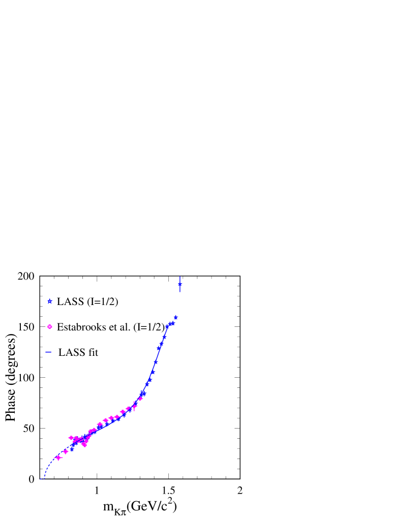
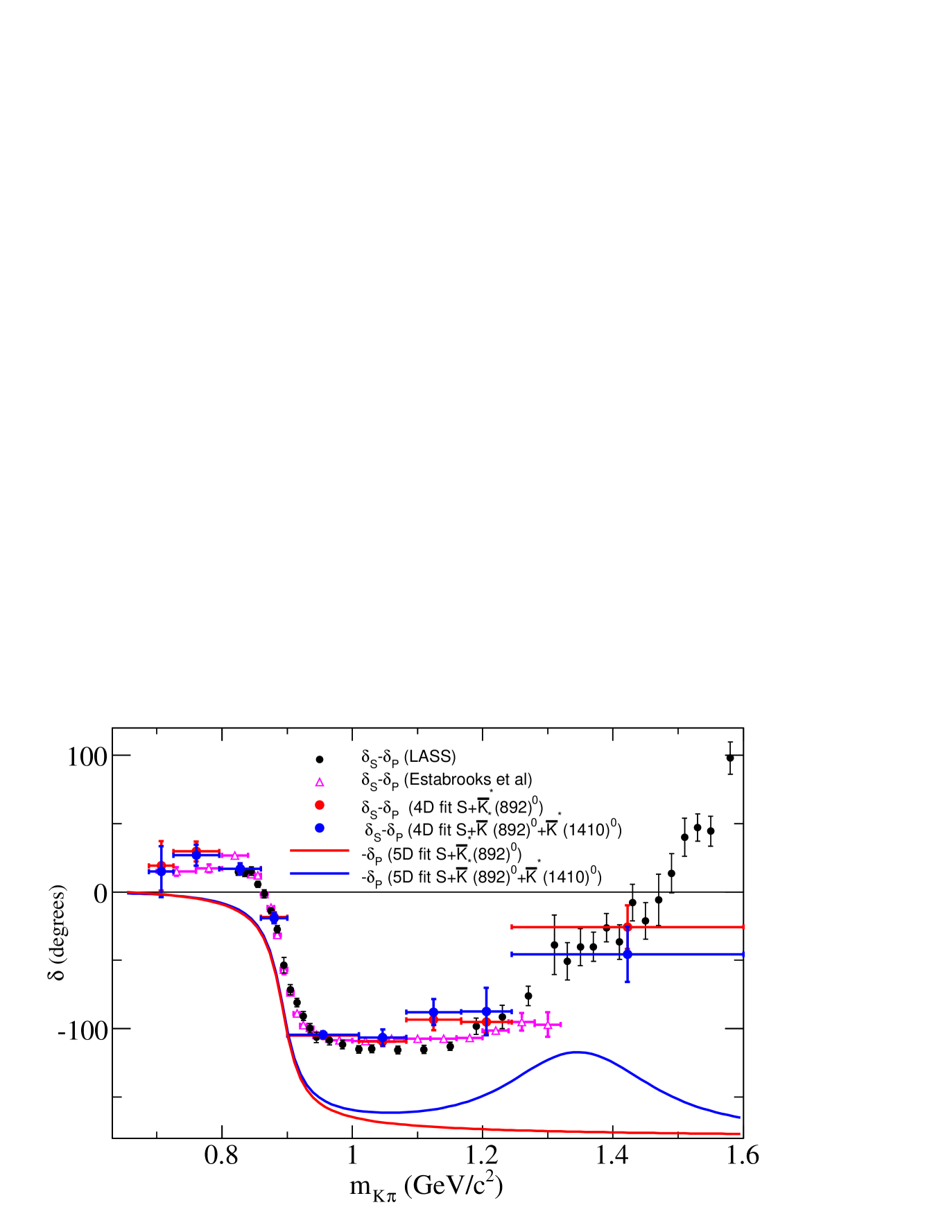
A $K\pi$ partial wave analysis of high statistics data for the reactions $K^{\pm}p\rightarrow K^{\pm}\pi^{+}n$ and $K^{\pm}p\rightarrow K^{\pm}\pi^{-}\Delta^{++}$ at 13 $\mathrm{\,Ge\kern-1.00006ptV}$ , on events selected at small momentum transfer ref:easta1 , provided information on $K\pi$ scattering for $m_{K\pi}$ in the range $[0.7,~1.9]~{\mathrm{\,Ge\kern-1.00006ptV\!/}c^{2}}$ . The $I=3/2$ $K\pi$ scattering was studied directly from the analyses of $K^{+}p\rightarrow K^{+}\pi^{+}n$ and $K^{-}p\rightarrow K^{-}\pi^{-}\Delta^{++}$ reactions. The phase of the elastic amplitude $(\delta_{S}^{3/2})$ was measured and was used to extract the phase of the $I=1/2$ amplitude from measurements of $K^{-}\pi^{+}$ scattering. Values obtained for $\delta_{S}^{1/2}$ are displayed in Fig. 1 for $m_{K\pi}<1.3~{\mathrm{\,Ge\kern-1.00006ptV\!/}c^{2}}$ , a mass range in which the interaction is expected to remain elastic. Above $1.46~{\mathrm{\,Ge\kern-1.00006ptV\!/}c^{2}}$ there were several solutions for the amplitude.

A few years later, the LASS experiment analyzed data from 11 ${\mathrm{\,Ge\kern-1.00006ptV\!/}c}$ kaon scattering on hydrogen: $K^{-}p\rightarrow K^{-}\pi^{+}n$ ref:lass1 . They performed a partial wave analysis of $1.5\times 10^{5}$ events which satisfied cuts to ensure $K\pi$ production dominated by pion exchange and no excitation of the target into baryon resonances.

The $K\pi$ , $I=1/2$ , $S$ -wave was parameterized as the sum of a background term $(BG)$ and the $K^{*}_{0}(1430)$ , which were combined such that the resulting amplitude satisfied unitarity:

$\displaystyle A_{S}^{1/2}$	$\displaystyle=$	$\displaystyle\sin{\delta_{BG}^{1/2}}\,e^{i\delta_{BG}^{1/2}}$
	$\displaystyle+$	$\displaystyle e^{2i\delta_{BG}^{1/2}}\sin{\delta_{K^{}_{0}(1430)}}\,e^{i\delta_{K^{}_{0}(1430)}}$
	$\displaystyle=$	$\displaystyle\sin{\left(\delta_{BG}^{1/2}+\delta_{K^{}_{0}(1430)}\right)}e^{i\left(\delta_{BG}^{1/2}+\delta_{K^{}_{0}(1430)}\right)},$

where $\delta_{BG}^{1/2}$ and $\delta_{K^{*}_{0}(1430)}$ depended on the $K\pi$ mass.

The mass dependence of $\delta_{BG}^{1/2}$ was described by means of an effective range parameterization:

\cot{(\delta_{BG}^{1/2})}=\frac{1}{a_{S,BG}^{1/2}~p^{*}}+\frac{b_{S,BG}^{1/2}~p^{*}}{2},

(8)

where $a_{S,BG}^{1/2}$ is the scattering length and $b_{S,BG}^{1/2}$ is the effective range. Note that these two parameters are different from $a_{\ell}^{I}$ and $b_{\ell}^{I}$ introduced in Eq. (3) as the latter referred to the total amplitude and also because Eq. (8) corresponds to an expansion near threshold which differs from Eq. (5). The mass dependence of $\delta_{K^{*}_{0}(1430)}$ was obtained assuming that the $K^{*}_{0}(1430)$ decay amplitude obeys a Breit-Wigner distribution:

\cot{(\delta_{K^{*}_{0}(1430)})}=\frac{m_{K^{*}_{0}(1430)}^{2}-m_{K\pi}^{2}}{m_{K^{*}_{0}(1430)}\Gamma_{K^{*}_{0}(1430)}(m_{K\pi})},

(9)

where $m_{K^{*}_{0}(1430)}$ is the pole mass of the resonance and $\Gamma_{K^{*}_{0}(1430)}(m_{K\pi})$ its mass-dependent total width.

The total $I=1/2$ $S$ -wave phase was then:

\delta_{LASS}^{1/2}=\delta_{BG}^{1/2}+\delta_{K^{*}_{0}(1430)}

(10)

The LASS measurements were based on fits to moments of angular distributions which depended on the interference between $S$ -, $P$ -, $D$ -…waves. To obtain the $I=1/2$ $K^{-}\pi^{+}$ $S$ -wave amplitude, the measured $I=3/2$ component ref:easta1 was subtracted from the LASS measurement of $T_{K^{-}\pi^{+}}$ and the resulting values were fitted using Eq. (10). The corresponding results ref:Dunwoodie are given in Table 3 and displayed in Fig. 1.

Table 3: Fit results to LASS data ref:Dunwoodie for two mass intervals.

Parameter	$m_{K\pi}\in[0.825,~1.52]$	$m_{K\pi}\in[0.825,~1.60]$
	${\mathrm{\,Ge\kern-1.00006ptV\!/}c^{2}}$	${\mathrm{\,Ge\kern-1.00006ptV\!/}c^{2}}$
$m_{K^{*}_{0}(1430)}~({\mathrm{\,Me\kern-1.00006ptV\!/}c^{2}})$	$1435\pm 5$	$1415\pm 3$
$\Gamma_{K^{*}_{0}(1430)}~({\mathrm{\,Me\kern-1.00006ptV\!/}c^{2}})$	$279\pm 6$	$300\pm 6$
$a_{S,BG}^{1/2}~(\mathrm{\,Ge\kern-1.00006ptV}^{-1})$	$1.95\pm 0.09$	$2.07\pm 0.10$
$b_{S,BG}^{1/2}~(\mathrm{\,Ge\kern-1.00006ptV}^{-1})$	$1.76\pm 0.36$	$3.32\pm 0.34$

Refer to caption — Figure 1: (color online) Comparison between the $I=1/2$ $S$ -wave phase measured in $K\pi$ production at small transfer for several values of the $K\pi$ mass. Results from Ref. ref:easta1 are limited to $m_{K\pi}<1.3~{\mathrm{\,Ge\kern-1.00006ptV\!/}c^{2}}$ to remain in the elastic regime where there is a single solution for the amplitude. The curve corresponds to the fit given in the second column of Table 3.

III.2 $\tau^{-}\rightarrow K\pi\nu_{\tau}$ decays

The BABAR and Belle collaborations ref:taubabar ; ref:taubelle measured the $K^{0}_{\scriptscriptstyle S}\pi$ mass distribution in $\tau^{-}\rightarrow K^{0}_{\scriptscriptstyle S}\pi^{-}\nu_{\tau}$ . Results from Belle were analyzed in Ref. ref:taupich1 using, in addition to the $K^{*}(892)$ :

•

a contribution from the $K^{*}(1410)$ to the vector form factor;
•

a scalar contribution, with a mass dependence compatible with LASS measurements but whose branching fraction was not provided.

Another interpretation of these data was given in Ref. ref:mouss2 . Using the value of the rate determined from Belle data, for the $K^{*}(1410)$ , its relative contribution to the $D^{+}\rightarrow K^{-}\pi^{+}e^{+}\nu_{e}$ channel was evaluated to be of the order of $0.5\%$ .

III.3 Hadronic $D$ meson decays

$K\pi$ interactions were studied in several Dalitz plot analyses of three-body $D$ decays and we consider only $D^{+}\rightarrow K^{-}\pi^{+}\pi^{+}$ as measured by the E791 ref:e791kpipi , FOCUS ref:focuskpipi ; ref:focuskpipi2 , and CLEO-c ref:kpipi_cleoc collaborations. This final state is known to have a large $S$ -wave component because there is no resonant contribution to the $\pi^{+}\pi^{+}$ system. In practice each collaboration has developed various approaches and results are difficult to compare.

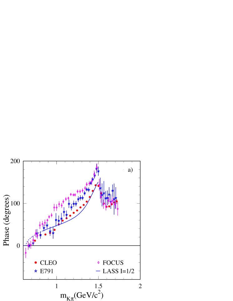
The $S$ -wave phase measured by these collaborations is compared in Fig. 2-a with the phase of the ( $I=1/2$ ) amplitude determined from LASS data. Measurements from $D^{+}$ decays are shifted so that the phase is equal to zero for $m_{K\pi}=0.67~{\mathrm{\,Ge\kern-1.00006ptV\!/}c^{2}}$ . The magnitude of the amplitude obtained in Dalitz plot analyses is compared in Fig. 2-b with the “naive” estimate given in Eq. (4), which is derived from the elastic ( $I=1/2$ ) amplitude fitted to LASS data.

By comparing results obtained by the three experiments analyzing $D^{+}\rightarrow K^{-}\pi^{+}\pi^{+}$ , several remarks are formulated.

•

A $\pi^{+}\pi^{+}$ component is included only in the CLEO-c measurement and it corresponds to $(15\pm 3)\%$ of the decay rate.
•

The relative importance of $I=1/2$ and $I=3/2$ components can be different in $K\pi$ scattering and in a three-body decay. This is because, even if Watson’s theorem is expected to be valid, it applies separately for the $I=1/2$ and $I=3/2$ components and concerns only the corresponding phases of these amplitudes. In E791 and CLEO-c they measured the total $K\pi$ $S$ -wave amplitude and compared their results with the $I=1/2$ component from LASS. FOCUS ref:focuskpipi , using the phase of the $I=3/2$ amplitude measured in scattering experiments, had fitted separately the two components and found large effects from the $I=3/2$ part. In Fig. 2-a the phase of the total $S$ -wave amplitude which contains contributions from the two isospin components, as measured by FOCUS ref:focuskpipi2 , is plotted.
•

Measured phases in Dalitz plot analyses have a global shift as compared to the scattering case (in which phases are expected to be zero at threshold). Having corrected for this effect (with some arbitrariness), the variation measured for the phase in three-body decays and in $K\pi$ scattering is roughly similar, but quantitative comparison is difficult. Differences between the two approaches as a function of $m_{K\pi}$ are much larger than the quoted uncertainties. They may arise from the comparison itself, which considers the total $K\pi$ $S$ -wave in one case and only the $I=1/2$ component for scattering. They could be due also to the interaction of the bachelor pion which invalidates the application of the Watson theorem.

It is thus difficult to draw quantitative conclusions from results obtained with $D^{+}\rightarrow K^{-}\pi^{+}\pi^{+}$ decays. Qualitatively, one can say that the phase of the $S$ -wave component depends roughly similarly on $m_{K\pi}$ as the phase measured by LASS. Below the $K^{*}_{0}(1430)$ , the $S$ -wave amplitude magnitude has a smooth variation versus $m_{K\pi}$ . At the $K^{*}_{0}(1430)$ average mass value and above, this magnitude has a sharp decrease with the mass.

III.4 $D_{\ell 4}$ decays

The dominant hadronic contribution in the $D_{\ell 4}$ decay channel comes from the ( $J^{P}$ = $1^{-}$ ) $K^{*}(892)$ resonant state. E687 ref:e687 gave the first suggestion for an additional component. FOCUS ref:focus1 , a few years later, measured the $S$ -wave contribution from the asymmetry in the angular distribution of the $K$ in the $K\pi$ rest frame. They concluded that the phase difference between $S$ - and $P$ -waves was compatible with a constant equal to $\pi/4$ , over the $K^{*}(892)$ mass region.

In the second publication ref:focus2 they found that the asymmetry could be explained if they used the variation of the $S$ -wave component versus the $K\pi$ mass measured by the LASS collaboration ref:lass1 . They did not fit to their data the two parameters that governed this phase variation but took LASS results:

$\displaystyle\cot{(\delta_{BG})}$	$\displaystyle=$	$\displaystyle\frac{1}{a_{S,BG}~p^{}}+\frac{b_{S,BG}~p^{}}{2},$	(11)
$\displaystyle a_{S,BG}$	$\displaystyle=$	$\displaystyle(4.03\pm 1.72\pm 0.06)~\mathrm{\,Ge\kern-1.00006ptV}^{-1},$
$\displaystyle b_{S,BG}$	$\displaystyle=$	$\displaystyle(1.29\pm 0.63\pm 0.67)~\mathrm{\,Ge\kern-1.00006ptV}^{-1}.$

These values corresponded to the total $S$ -wave amplitude measured by LASS which was the sum of $I=1/2$ and $I=3/2$ contributions whereas only the former component was present in charm semileptonic decays. For the $S$ -wave amplitude they assumed that it was proportional to the elastic amplitude (see Eq. (4)). For the $P$ -wave, they used a relativistic Breit-Wigner with mass dependent width ref:angles . They fitted the values of the pole mass, the width and the Blatt-Weisskopf damping parameter for the $K^{*}(892)$ . These values from FOCUS are given in Table 4 and compared with present world averages ref:pdg10 . , dominated by the $P$ -wave measurements from LASS.

Table 4: Parameters of the

K^{*}(892)^{0}

measured by FOCUS are compared with world average or previous values.

Parameter	FOCUS results ref:focus2	previous results
$m_{K^{*0}}~({\mathrm{\,Me\kern-1.00006ptV\!/}c^{2}})$	$895.41\pm 0.32^{+0.35}_{-0.43}$	$895.94\pm 0.22$ ref:pdg10
$\Gamma_{K^{*0}}^{0}~({\mathrm{\,Me\kern-1.00006ptV\!/}c^{2}})$	$~47.79\pm 0.86^{+1.32}_{-1.06}$	$~48.7\pm 0.8$ ref:pdg10
$r_{BW}~({\mathrm{\,Ge\kern-1.00006ptV\!/}c})^{-1}$	$~~3.96\pm 0.54^{+1.31}_{-0.90}$	$~3.40\pm 0.67$ ref:lass1

They also compared the measured angular asymmetry of the $K$ in the $K\pi$ rest frame versus the $K\pi$ mass with expectations from a $\kappa$ resonance and conclude that the presence of a $\kappa$ could be neglected. They used a Breit-Wigner distribution for the $\kappa$ amplitude using values measured by the E791 collaboration ref:e791kappa for the mass and width of this resonance ( $m_{\kappa}=797\pm 19\pm 43~{\mathrm{\,Me\kern-1.00006ptV\!/}c^{2}},~\Gamma_{\kappa}=410\pm 43\pm 87~{\mathrm{\,Me\kern-1.00006ptV\!/}c^{2}}$ ). This approach to search for a $\kappa$ does not seem to be appropriate. Adding a $\kappa$ in this way violates the Watson theorem as the phase of the fitted $K\pi$ amplitude would differ greatly from the one measured by LASS. In addition, the interpretation of LASS measurements in Ref. ref:seb1 concluded there was evidence for a $\kappa$ . In addition to the $K^{*}(892)$ they measured the rate for the non-resonant $S$ -wave contribution and placed limits on other components (Table 5).

Table 5: Measured fraction of the non-resonant

S

-wave component and limits on contributions from

K^{*}_{0}(1430)

and

K^{*}(1680)

in the decay

D^{+}\rightarrow K^{-}\pi^{+}\mu^{+}\nu_{\mu}

, obtained by FOCUS ref:focus2 .

Channel	FOCUS ref:focus2 ( $\%$ )
$\frac{\Gamma(D^{+}\rightarrow K^{-}\pi^{+}\mu^{+}\nu_{\mu})_{NR}}{\Gamma(D^{+}\rightarrow K^{-}\pi^{+}\mu^{+}\nu_{\mu})}$	$5.30\pm 0.74^{+0.99}_{-0.96}$
$\frac{\Gamma(D^{+}\rightarrow K^{-}\pi^{+}\mu^{+}\nu_{\mu})_{K^{*}_{0}(1430)}}{\Gamma(D^{+}\rightarrow K^{-}\pi^{+}\mu^{+}\nu_{\mu})}$	$<0.64\%~{\rm at}~90\%$ C.L.
$\frac{\Gamma(D^{+}\rightarrow K^{-}\pi^{+}\mu^{+}\nu_{\mu})_{K^{*}(1680)}}{\Gamma(D^{+}\rightarrow K^{-}\pi^{+}\mu^{+}\nu_{\mu})}$	$<4.0\%~{\rm at}~90\%$ C.L.

Analyzing $D^{+}\rightarrow K^{-}\pi^{+}e^{+}\nu_{e}$ events from a sample corresponding to $281~{\rm pb}^{-1}$ integrated luminosity, the CLEO-c collaboration had confirmed the FOCUS result for the $S$ -wave contribution. They did not provide an independent measurement of the $S$ -wave phase ref:cleoc1 .

IV $D^{+}\rightarrow K^{-}\pi^{+}e^{+}\nu_{e}$ decay rate formalism

The invariant matrix element for the $D^{+}\rightarrow K^{-}\pi^{+}e^{+}\nu_{e}$ semileptonic decay is the product of a hadronic and a leptonic current.

	$\displaystyle{\cal M}_{fi}$	$\displaystyle=$	$\displaystyle\frac{G_{F}}{\sqrt{2}}\|V_{cs}\|\left<\pi(p_{\pi^{+}})K(p_{K^{-}})\|\overline{s}\gamma_{\mu}(1-\gamma_{5})c\|D(p_{D^{+}})\right>$		(12)
			$\displaystyle\times\overline{u}(p_{\nu_{e}})\gamma_{\mu}(1-\gamma_{5})v(p_{e^{+}}).$		(12)

In this expression, $p_{K^{-}},~p_{\pi^{+}},~p_{e^{+}}~{\rm and}~p_{\nu_{e}}$ are the $K^{-},~\pi^{+},~e^{+}$ , and $\nu_{e}$ four-momenta, respectively.

The leptonic current corresponds to the virtual $W^{+}$ which decays into $e^{+}\nu_{e}$ . The matrix element of the hadronic current can be written in terms of four form factors, but neglecting the electron mass, only three are contributing to the decay rate: $h$ and $w_{\pm}$ . Using the conventions of Ref. ref:wise1 , the vector and axial-vector components are, respectively:

	$\displaystyle\left<\pi(p_{\pi^{+}})K(p_{K^{-}})\|\overline{s}\gamma_{\mu}c\|D(p_{D^{+}})\right>~~~~~~~~~~~~~~~~~~~~~~$
	$\displaystyle=h\epsilon_{\mu\alpha\beta\gamma}p_{D^{+}}^{\alpha}\left(p_{K^{-}}+p_{\pi^{+}}\right)^{\beta}\left(p_{K^{-}}-p_{\pi^{+}}\right)^{\gamma};$		(13)
	$\displaystyle\left<\pi(p_{\pi^{+}})K(p_{K^{-}})\|\overline{s}\gamma_{\mu}(-\gamma_{5})c\|D(p_{D^{+}})\right>~~~~~~~~~~~~~~~$
	$\displaystyle=iw_{+}\left(p_{K^{-}}+p_{\pi^{+}}\right)_{\mu}+iw_{-}\left(p_{K^{-}}-p_{\pi^{+}}\right)_{\mu}.~$		(14)

As there are 4 particles in the final state, the differential decay rate has five degrees of freedom that can be expressed in the following variables ref:cab1 ; ref:pais1 :

•

$m^{2}$ , the mass squared of the $K\pi$ system;
•

$q^{2}$ , the mass squared of the $e^{+}\nu_{e}$ system;
•

$\cos{(\theta_{K})}$ , where $\theta_{K}$ is the angle between the $K$ three-momentum in the $K\pi$ rest frame and the line of flight of the $K\pi$ in the $D$ rest frame;
•

$\cos{(\theta_{e})}$ , where $\theta_{e}$ is the angle between the charged lepton three-momentum in the $e\nu_{e}$ rest frame and the line of flight of the $e\nu_{e}$ in the $D$ rest frame;
•

$\chi$ , the angle between the normals to the planes defined in the $D$ rest frame by the $K\pi$ pair and the $e\nu_{e}$ pair. $\chi$ is defined between $-\pi$ and $+\pi$ .

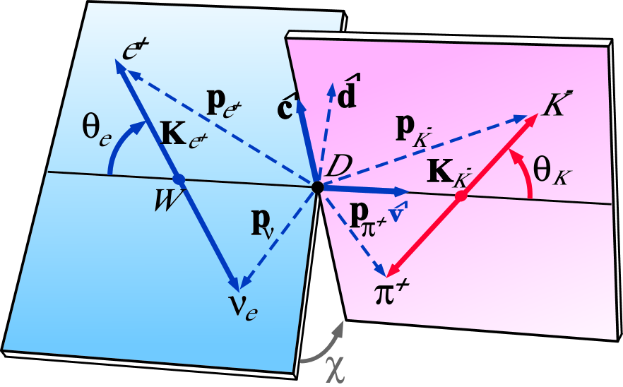
The angular variables are shown in Fig. 3, where $\mbox{\boldmath{$K$}}_{K^{-}}$ is the $K^{-}$ three-momentum in the $K\pi$ CM and $\mbox{\boldmath{$K$}}_{e^{+}}$ is the three-momentum of the positron in the virtual $W$ CM. Let $\hat{\mbox{\boldmath{$v$}}}$ be the unit vector along the $K\pi$ direction in the $D$ rest frame, $\hat{\mbox{\boldmath{$c$}}}$ the unit vector along the projection of $\mbox{\boldmath{$K$}}_{K^{-}}$ perpendicular to $\hat{\mbox{\boldmath{$v$}}}$ , and $\hat{\mbox{\boldmath{$d$}}}$ the unit vector along the projection of $\mbox{\boldmath{$K$}}_{e^{+}}$ perpendicular to $\hat{\mbox{\boldmath{$v$}}}$ . We have:

	$\displaystyle m^{2}=(p_{\pi^{+}}+p_{K^{-}})^{2},~q^{2}=(p_{e^{+}}+p_{\nu_{e}})^{2},$		(15)
	$\displaystyle\cos{(\theta_{K})}=\frac{\hat{\mbox{\boldmath{$v$}}}\cdot\mbox{\boldmath{$K$}}_{K^{-}}}{\|\mbox{\boldmath{$K$}}_{K^{-}}\|},~\cos{(\theta_{e})}=-\frac{\hat{\mbox{\boldmath{$v$}}}\cdot\mbox{\boldmath{$K$}}_{e^{+}}}{\|\mbox{\boldmath{$K$}}_{e^{+}}\|},$
	$\displaystyle\cos{(\chi)}=\hat{\mbox{\boldmath{$c$}}}\cdot\hat{\mbox{\boldmath{$d$}}};\;\;\sin{(\chi)}=(\hat{\mbox{\boldmath{$c$}}}\times\hat{\mbox{\boldmath{$v$}}})\cdot\hat{\mbox{\boldmath{$d$}}}$

The definition of $\chi$ is the same as proposed initially in Ref. ref:cab1 . When analyzing $D^{-}$ decays, the sign of $\chi$ has to be changed. This is because, if $C\!P$ invariance is assumed with the adopted definitions, $\chi$ changes sign through $C\!P$ transformation of the final state ref:focus1 .

For the differential decay partial width, we use the formalism given in Ref. ref:wise1 , which generalizes to five variables the decay rate given in Ref. ref:rich1 in terms of $q^{2},~\cos\theta_{K},~\cos\theta_{e}$ and $\chi$ variables. In addition, it provides a partial wave decomposition for the hadronic system. Any dependence on the lepton mass is neglected as only electrons or positrons are used in this analysis:

	$\displaystyle{\rm d}^{5}\Gamma=\frac{G_{F}^{2}\left\|\|V_{cs}\|\right\|^{2}}{\left(4\pi\right)^{6}m_{D}^{3}}X\beta{\cal I}(m^{2},q^{2},\theta_{K},\theta_{e},\chi)$
	$\displaystyle{\rm d}m^{2}{\rm d}q^{2}{\rm d}\cos{(\theta_{K})}{\rm d}\cos{(\theta_{e})}{\rm d}\chi.$		(16)

In this expression, $X=p_{K\pi}\,m_{D}$ where $p_{K\pi}$ is the momentum of the $K\pi$ system in the $D$ rest frame, and $\beta=2p^{*}/m$ . $p^{*}$ is the breakup momentum of the $K\pi$ system in its rest frame. The form factors $h$ and $w_{\pm}$ , introduced in Eq. (13-14), are functions of $m^{2}$ , $q^{2}$ and $\cos{\theta_{K}}$ . In place of these form factors and to simplify the notations, the quantities ${\cal F}_{1,2,3}$ are defined ref:wise1 :

$\displaystyle{\cal F}_{1}$	$\displaystyle=$	$\displaystyle Xw_{+}+\left[\beta(p_{K^{-}}+p_{\pi^{+}})(p_{e^{+}}+p_{\nu_{e}})\cos{\theta_{K}}\right.$
	$\displaystyle+$	$\displaystyle\left.\frac{m_{K}^{2}-m_{\pi}^{2}}{m^{2}}X\right]w_{-},$
$\displaystyle{\cal F}_{2}$	$\displaystyle=$	$\displaystyle\beta\,q\,m\,w_{-},$	(17)
$\displaystyle{\cal F}_{3}$	$\displaystyle=$	$\displaystyle\beta\,X\,q\,m\,h.$

The dependence of ${\cal I}$ on $\theta_{e}$ and $\chi$ is given by:

$\displaystyle{\cal I}$	$\displaystyle=$	$\displaystyle{\cal I}_{1}+{\cal I}_{2}\cos{2\theta_{e}}+{\cal I}_{3}\sin^{2}{\theta_{e}}\cos{2\chi}$
		$\displaystyle+{\cal I}_{4}\sin{2\theta_{e}}\cos{\chi}+{\cal I}_{5}\sin{\theta_{e}}\cos{\chi}$
		$\displaystyle+{\cal I}_{6}\cos{\theta_{e}}+{\cal I}_{7}\sin{\theta_{e}}\sin{\chi}$
		$\displaystyle+{\cal I}_{8}\sin{2\theta_{e}}\sin{\chi}+{\cal I}_{9}\sin^{2}{\theta_{e}}\sin{2\chi}$

where ${\cal I}_{1,...,9}$ depend on $m^{2},~q^{2}$ and $\theta_{K}$ . These quantities can be expressed in terms of the three form factors, ${\cal F}_{1,2,3}$ .

$\displaystyle{\cal I}_{1}$	$\displaystyle=$	$\displaystyle\frac{1}{4}\left\{\|{\cal F}_{1}\|^{2}+\frac{3}{2}\sin^{2}{\theta_{K}}\left(\|{\cal F}_{2}\|^{2}+\|{\cal F}_{3}\|^{2}\right)\right\}$	(19)
$\displaystyle{\cal I}_{2}$	$\displaystyle=$	$\displaystyle-\frac{1}{4}\left\{\|{\cal F}_{1}\|^{2}-\frac{1}{2}\sin^{2}{\theta_{K}}\left(\|{\cal F}_{2}\|^{2}+\|{\cal F}_{3}\|^{2}\right)\right\}$
$\displaystyle{\cal I}_{3}$	$\displaystyle=$	$\displaystyle-\frac{1}{4}\left\{\|{\cal F}_{2}\|^{2}-\|{\cal F}_{3}\|^{2}\right\}\sin^{2}{\theta_{K}}$
$\displaystyle{\cal I}_{4}$	$\displaystyle=$	$\displaystyle\frac{1}{2}{\rm Re}\left({\cal F}_{1}^{*}{\cal F}_{2}\right)\sin{\theta_{K}}$
$\displaystyle{\cal I}_{5}$	$\displaystyle=$	$\displaystyle{\rm Re}\left({\cal F}_{1}^{*}{\cal F}_{3}\right)\sin{\theta_{K}}$
$\displaystyle{\cal I}_{6}$	$\displaystyle=$	$\displaystyle{\rm Re}\left({\cal F}_{2}^{*}{\cal F}_{3}\right)\sin^{2}{\theta_{K}}$
$\displaystyle{\cal I}_{7}$	$\displaystyle=$	$\displaystyle{\rm Im}\left({\cal F}_{1}{\cal F}_{2}^{*}\right)\sin{\theta_{K}}$
$\displaystyle{\cal I}_{8}$	$\displaystyle=$	$\displaystyle\frac{1}{2}{\rm Im}\left({\cal F}_{1}{\cal F}_{3}^{*}\right)\sin{\theta_{K}}$
$\displaystyle{\cal I}_{9}$	$\displaystyle=$	$\displaystyle-\frac{1}{2}{\rm Im}\left({\cal F}_{2}{\cal F}_{3}^{*}\right)\sin^{2}{\theta_{K}}$

Form factors ${\cal F}_{1,2,3}$ can be expanded into partial waves to show their explicit dependence on $\theta_{K}$ . If only $S$ -, $P$ - and $D$ -waves are kept, this gives:

$\displaystyle{\cal F}_{1}$	$\displaystyle=$	$\displaystyle{\cal F}_{10}+{\cal F}_{11}\cos{\theta_{K}}+{\cal F}_{12}\frac{3\cos^{2}{\theta_{K}}-1}{2};$
$\displaystyle{\cal F}_{2}$	$\displaystyle=$	$\displaystyle\frac{1}{\sqrt{2}}{\cal F}_{21}+\sqrt{\frac{3}{2}}{\cal F}_{22}\cos{\theta_{K}};$	(20)
$\displaystyle{\cal F}_{3}$	$\displaystyle=$	$\displaystyle\frac{1}{\sqrt{2}}{\cal F}_{31}+\sqrt{\frac{3}{2}}{\cal F}_{32}\cos{\theta_{K}}.$

Form factors ${\cal F}_{ij}$ depend on $m^{2}$ and $q^{2}$ . ${\cal F}_{10}$ characterizes the $S$ -wave contribution whereas ${\cal F}_{i1}$ and ${\cal F}_{i2}$ correspond to the $P$ - and $D$ -wave, respectively.

IV.1 $P$ -wave form factors

By comparing expressions given in Ref. ref:wise1 and ref:rich1 it is possible to relate ${\cal F}_{i1},~i=1,2,3$ with the helicity form factors $H_{0,\pm}$ :

$\displaystyle{\cal F}_{11}$	$\displaystyle=$	$\displaystyle 2\sqrt{2}\alpha\,q\,H_{0}$
$\displaystyle{\cal F}_{21}$	$\displaystyle=$	$\displaystyle 2\alpha\,q\left(H_{+}+H_{-}\right)$	(21)
$\displaystyle{\cal F}_{31}$	$\displaystyle=$	$\displaystyle 2\alpha\,q\left(H_{+}-H_{-}\right)$

where $\alpha$ is a constant factor, its value is given in Eq. (26); it depends on the definition adopted for the mass distribution. The helicity amplitudes can in turn be related to the two axial-vector form factors $A_{1,2}(q^{2})$ , and to the vector form factor $V(q^{2})$ :

$\displaystyle H_{0}(q^{2})$	$\displaystyle=$	$\displaystyle\frac{1}{2m\,q}\left[\left(m_{D}^{2}-m^{2}-q^{2}\right)\left(m_{D}+m\right)A_{1}(q^{2})\right.$	(22)
	$\displaystyle-$	$\displaystyle\left.4\frac{m_{D}^{2}\,p_{K\pi}^{2}}{m_{D}+m}A_{2}(q^{2})\right]$	(22)
$\displaystyle H_{\pm}(q^{2})$	$\displaystyle=$	$\displaystyle\left(m_{D}+m\right)A_{1}(q^{2})\mp\frac{2m_{D}\,p_{K\pi}}{m_{D}+m}V(q^{2}).$

As we are considering resonances which have an extended mass distribution, form factors can also have a mass dependence. We have assumed that the $q^{2}$ and $m$ dependence can be factorized:

(V,A_{1},A_{2})(q^{2},m)=(V,A_{1},A_{2})(q^{2})\times{\cal A}(m)

(23)

where in case of a resonance ${\cal A}(m)$ is assumed to behave according to a Breit-Wigner distribution.

This factorized expression can be justified by the fact that the $q^{2}$ dependence of the form factors is expected to be determined by the singularities which are nearest to the physical region: $q^{2}\in[0,~q^{2}_{max}]$ . These singularities are poles or cuts situated at (or above) hadron masses $M_{H}\simeq 2.1$ - $2.5~{\mathrm{\,Ge\kern-1.00006ptV\!/}c^{2}}$ , depending on the form factor. Because the $q^{2}$ variation range is limited to $q^{2}\simeq 1~\mathrm{\,Ge\kern-1.00006ptV}^{2}$ , the proposed approach is equivalent to an expansion in $q^{2}/M_{H}^{2}<0.2$ .

For the $q^{2}$ dependence we use a single pole parameterization and try to determine the effective pole mass.

$\displaystyle V(q^{2})$	$\displaystyle=$	$\displaystyle\frac{V(0)}{1-\frac{q^{2}}{m_{V}^{2}}}$
$\displaystyle A_{1}(q^{2})$	$\displaystyle=$	$\displaystyle\frac{A_{1}(0)}{1-\frac{q^{2}}{m_{A}^{2}}}$	(24)
$\displaystyle A_{2}(q^{2})$	$\displaystyle=$	$\displaystyle\frac{A_{2}(0)}{1-\frac{q^{2}}{m_{A}^{2}}}$

where $m_{V}$ and $m_{A}$ are expected to be close to $m_{D^{*}_{s}}\simeq 2.1~{\mathrm{\,Ge\kern-1.00006ptV\!/}c^{2}}$ and $m_{D_{s1}}\simeq 2.5~{\mathrm{\,Ge\kern-1.00006ptV\!/}c^{2}}$ respectively. Other parameterizations involving a double pole in $V$ have been proposed ref:doublepole , but as the present analysis is not sensitive to $m_{V}$ , the single pole ansatz is adequate.

Ratios of these form factors, evaluated at $q^{2}=0$ , $r_{V}=\frac{V(0)}{A_{1}(0)}$ and $r_{2}=\frac{A_{2}(0)}{A_{1}(0)}$ , are measured by studying the variation of the differential decay rate versus the kinematic variables. The value of $A_{1}(0)$ is determined by measuring the $D^{+}\rightarrow\overline{K}^{*0}e^{+}\nu_{e}$ branching fraction. For the mass dependence, in case of the $K^{*}(892)$ , we use a Breit-Wigner distribution:

{\cal A}_{K^{*}(892)}=\frac{m_{K^{*}(892)}\Gamma_{K^{*}(892)}^{0}F_{1}(m)}{m_{K^{*}(892)}^{2}-m^{2}-im_{K^{*}(892)}\Gamma_{K^{*}(892)}(m)}.

(25)

In this expression:

•

$m_{K^{*}(892)}$ is the $K^{*}(892)$ pole mass;
•

$\Gamma_{K^{*}(892)}^{0}$ is the total width of the $K^{*}(892)$ for $m=m_{K^{*}(892)}$ ;
•

$\Gamma_{K^{*}(892)}(m)$ is the mass-dependent $K^{*}(892)$ width: $\Gamma_{K^{*}(892)}(m)=\Gamma_{K^{*}(892)}^{0}\frac{p^{*}}{p^{*}_{0}}\frac{m_{K^{*}(892)}}{m}F^{2}_{1}(m)$ ;
•

$F_{1}(m)=\frac{p^{*}}{p^{*}_{0}}\frac{B(p^{*})}{B(p^{*}_{0})}$ where $B$ is the Blatt-Weisskopf damping factor: $B=1/\sqrt{1+r_{BW}^{2}p^{*2}}$ , $r_{BW}$ is the barrier factor, $p^{*}$ and $p^{*}_{0}$ are evaluated at the mass $m$ and $m_{K^{*}(892)}$ respectively and depend also on the masses of the $K^{*}(892)$ decay products.

With the definition of the mass distribution given in Eq. (25), the parameter $\alpha$ entering in Eq. (21) is equal to:

\alpha=\sqrt{\frac{3\pi B_{K^{*}}}{p^{*}_{0}~\Gamma_{K^{*}(892)}^{0}}}

(26)

where $B_{K^{*}}={\cal B}\left(K^{*}(892)\rightarrow K^{-}\pi^{+}\right)=2/3$ .

IV.2 $S$ -wave form factor

In a similar way as for the $P$ -wave, we need to have the correspondence between the $S$ -wave amplitude ${\cal F}_{10}$ (Eq. (IV)) and the corresponding invariant form factor. In an $S$ -wave, only the helicity $H_{0}$ form factor can contribute and we take:

{\cal F}_{10}=p_{K\pi}m_{D}\frac{1}{1-\frac{q^{2}}{m_{A}^{2}}}{\cal A}_{S}(m).

(27)

The term ${\cal F}_{10}$ is proportional to $p_{K\pi}$ to ensure that the corresponding decay rate varies as $p_{K\pi}^{3}$ as expected from the $L=1$ angular momentum between the virtual $W$ and the $S$ -wave $K\pi$ hadronic state. Because the $q^{2}$ variation of the form factor is expected to be determined by the contribution of $J^{P}=1^{+}~c\bar{s}$ states, we use the same $q^{2}$ dependence as for $A_{1}$ and $A_{2}$ . The term ${\cal A}_{S}(m)$ corresponds to the mass dependent $S$ -wave amplitude. Considering that previous charm Dalitz plot analyses have measured an $S$ -wave amplitude magnitude which is essentially constant up to the $K_{0}^{*}(1430)$ mass and then drops sharply above this value, we have used the following ansatz:

$\displaystyle{\cal A}_{S}$	$\displaystyle=$	$\displaystyle r_{S}P(m)e^{i\delta_{S}(m)},~{\rm and}$	(28)
$\displaystyle{\cal A}_{S}$	$\displaystyle=$	$\displaystyle r_{S}P(m_{K^{*}_{0}(1430)})$
	$\displaystyle\times$	$\displaystyle\sqrt{\frac{(m_{K_{0}^{}(1430)}\Gamma_{K_{0}^{}(1430)})^{2}}{(m_{K_{0}^{}(1430)}^{2}-m^{2})^{2}+(m_{K_{0}^{}(1430)}\Gamma_{K_{0}^{*}(1430)})^{2}}}~e^{i\delta_{S}(m)},$

respectively for $m$ below and above the $K^{*}_{0}(1430)$ pole mass value. In these expressions, $\delta_{S}(m)$ is the $S$ -wave phase, $P(m)=1+r_{S}^{(1)}\times x+r_{S}^{(2)}\times x^{2}+...$ and $x=\sqrt{(\frac{m}{m_{K}+m_{\pi}})^{2}-1}$ . The coefficients $r^{(i)}_{S}$ have no dimension and their values are fitted, but in practice, the fit to data is sensitive only to the linear term. We have introduced the constant $r_{S}$ which measures the magnitude of the $S$ -wave amplitude. From the observed asymmetry of the $\cos{\theta_{K}}$ distribution in our data, $r_{S}<0$ . This relative sign between $S$ and $P$ waves agrees with the FOCUS measurement ref:focus1 .

IV.3 $D$ -wave form factors

Expressions for the form factors ${\cal F}_{i,2}$ for the $D$ -wave are ref:Seb_Dwave :

$\displaystyle{\cal F}_{12}$	$\displaystyle=$	$\displaystyle\frac{m_{D}\,p_{K\pi}}{3}\left[\left(m_{D}^{2}-m^{2}-q^{2}\right)\left(m_{D}+m\right)T_{1}(q^{2})\right.$
	$\displaystyle-$	$\displaystyle\left.\frac{m_{D}^{2}\,p_{K\pi}^{2}}{m_{D}+m}T_{2}(q^{2})\right],$
$\displaystyle{\cal F}_{22}$	$\displaystyle=$	$\displaystyle\sqrt{\frac{2}{3}}m_{D}\,m\,q\,p_{K\pi}\left(m_{D}+m\right)T_{1}(q^{2}),$	(29)
$\displaystyle{\cal F}_{32}$	$\displaystyle=$	$\displaystyle\sqrt{\frac{2}{3}}\frac{2m_{D}^{2}\,m\,q\,p^{2}_{K\pi}}{\left(m_{D}+m\right)}T_{V}(q^{2}).$

These expressions are multiplied by a relativistic Breit-Wigner amplitude which corresponds to the $K_{2}^{*}(1430)$ :

\displaystyle{{\cal A}_{K_{2}^{*}}=\frac{r_{D}\,m_{K_{2}^{*}(1430)}\Gamma_{K_{2}^{*}(1430)}^{0}F_{2}(m)}{m_{K_{2}^{*}(1430)}^{2}-m^{2}-im_{K_{2}^{*}(1430)}\Gamma_{K_{2}^{*}(1430)}(m)}.}

(30)

$r_{D}$ measures the magnitude of the $D$ -wave amplitude and similar conventions as in Eq. (25) are used for the other variables apart from the Blatt-Weisskopf term which is equal to:

\displaystyle B_{2}=1/\sqrt{\left(r_{BW}^{2}p^{*2}-3\right)^{2}+9r_{BW}^{2}p^{*2}},

(31)

and enters into

\displaystyle F_{2}(m)=\left(\frac{p^{*}}{p^{*}_{0}}\right)^{2}\frac{B_{2}(p^{*})}{B_{2}(p^{*}_{0})}.

(32)

The form factors $T_{i}(q^{2})$ ( $i=1,~2,~V$ ) are parameterized assuming the single pole model with corresponding axial or vector poles. Values for these pole masses are assumed to be the same as those considered before for the $S$ - or $P$ -wave hadronic form factors. Ratios of $D$ -wave hadronic form factors evaluated at $q^{2}=0$ , $r_{22}=T_{2}(0)/T_{1}(0)$ and $r_{2V}=T_{V}(0)/T_{1}(0)$ are supposed to be equal to one ref:dwave .

V The BABAR detector and dataset

A detailed description of the BABAR detector and of the algorithms used for charged and neutral particle reconstruction and identification is provided elsewhere ref:babar ; ref:babardet . Charged particles are reconstructed by matching hits in the five-layer double-sided silicon vertex tracker (SVT) with track elements in the 40 layer drift chamber (DCH), which is filled with a gas mixture of helium and isobutane. Slow particles which due to bending in the $1.5$ T magnetic field do not have enough hits in the DCH, are reconstructed in the SVT only. Charged hadron identification is performed combining the measurements of the energy deposition in the SVT and in the DCH with the information from the Cherenkov detector (DIRC). Photons are detected and measured in the CsI(Tl) electro-magnetic calorimeter (EMC). Electrons are identified by the ratio of the track momentum to the associated energy deposited in the EMC, the transverse profile of the shower, the energy loss in the DCH, and the Cherenkov angle in the DIRC. Muons are identified in the instrumented flux return, composed of resistive plate chambers and limited streamer tubes interleaved with layers of steel and brass.

The results presented here are obtained using a total integrated luminosity of $347.5~\mbox{\,fb}^{-1}$ . Monte Carlo (MC) simulation samples of $\mathchar 28935\relax{(4S)}$ decays, charm, and light quark pairs from continuum, equivalent to $3.3,~1.7,~{\rm and}~1.1$ times the data statistics, respectively, and have been generated using Geant4 ref:geant4 . These samples are used mainly to evaluate background components. Quark fragmentation in continuum events is described using the JETSET package ref:jetset . The MC distributions are rescaled to the data sample luminosity, using the expected cross sections of the different components : $1.3$ nb for $c\overline{c}$ , $0.525$ nb for $B^{+}B^{-}$ and $B^{0}\overline{B}^{0}$ , and $2.09$ nb for light $u\bar{u}$ , $d\bar{d}$ , and $s\bar{s}$ quark events. Dedicated samples of pure signal events, equivalent to 4.5 times the data statistics, are used to correct measurements for efficiency and finite resolution effects. Radiative decays $(D^{+}\rightarrow K^{-}\pi^{+}e^{+}\nu_{e}\gamma)$ are modeled by PHOTOS ref:photos . Events with a $D^{+}$ decaying into $K^{-}\pi^{+}\pi^{+}$ are also reconstructed in data and simulation. This control sample is used to adjust the $c$ -quark fragmentation distribution and the kinematic characteristics of particles accompanying the $D^{+}$ meson in order to better match the data. It is used also to measure the reconstruction accuracy of the missing neutrino momentum. Other samples with a $D^{0}$ , a $D^{*+}$ , or a $D^{+}_{s}$ meson exclusively reconstructed are used to define corrections on production characteristics of charm mesons and accompanying particles that contribute to the background.

VI Analysis method

Candidate signal events are isolated from $\mathchar 28935\relax{(4S)}$ and continuum events using variables combined into two Fisher discriminants, tuned to suppress $\mathchar 28935\relax{(4S)}$ and continuum background events, respectively. Several differences between distributions of quantities entering in the analysis, in data and simulation, are measured and corrected using dedicated event samples.

VI.1 Signal Selection

The approach used to reconstruct $D^{+}$ mesons decaying into $K^{-}\pi^{+}e^{+}\nu_{e}$ is similar to that used in previous analyses studying $D^{0}\rightarrow K^{-}e^{+}\nu_{e}$ ref:kenu and $D^{+}_{s}\rightarrow K^{+}K^{-}e^{+}\nu_{e}$ ref:kkenu . Charged and neutral particles are boosted to the CM system and the event thrust axis is determined. A plane perpendicular to this axis is used to define two hemispheres.

Signal candidates are extracted from a sample of events already enriched in charm semileptonic decays. Criteria applied for first enriching selection are:

•

an existence of a positron candidate with a momentum larger than $0.5~{\mathrm{\,Ge\kern-1.00006ptV\!/}c}$ in the CM frame, to eliminate most of light quark events. Positron candidates are accepted based on a tight identification selection with a pion misidentified as an electron or a positron below one per mill;
•

a value of $R_{2}>0.2$ , $R_{2}$ being the ratio between second- and zeroth-order Fox-Wolfram moments ref:r2 , to decrease the contribution from $B$ decays;
•

a minimum value for the invariant mass of the particles in the event hemisphere opposite to the electron candidate, $m_{opp}>0.5~{\mathrm{\,Ge\kern-1.00006ptV\!/}c^{2}}$ , to reject lepton pairs and two-photon events;
•

the invariant mass of the system formed by the positron and the most energetic particle in the candidate hemisphere, $m_{tag}>0.13~{\mathrm{\,Ge\kern-1.00006ptV\!/}c^{2}}$ , to remove events where the lepton is the only particle in its hemisphere.

A candidate is a positron, a charged kaon, and a charged pion present in the same hemisphere. A vertex is formed using these three tracks, and the corresponding $\chi^{2}$ probability larger than $10^{-7}$ are kept. The value of this probability is used in the following with other information to reject background events.

All other tracks in the hemisphere are defined as “spectators”. They most probably originate from the beam interaction point and are emitted during hadronization of the created $c$ and $\overline{c}$ quarks. The “leading” particle is the spectator particle having the highest momentum. Information from the spectator system is used to decrease the contribution from the combinatorial background. As charm hadrons take a large fraction of the charm quark energy, charm decay products have, on average, higher energies than spectator particles.

To estimate the neutrino momentum, the $(K^{-}\pi^{+}e^{+}\nu_{e})$ system is constrained to the $D^{+}$ mass. In this fit, estimates of the $D^{+}$ direction and of the neutrino energy are included from measurements obtained from all tracks registered in the event. The $D^{+}$ direction estimate is taken as the direction of the vector opposite to the momentum sum of all reconstructed particles but the kaon, the pion, and the positron. The neutrino energy is evaluated by subtracting from the hemisphere energy the energy of reconstructed particles contained in that hemisphere. The energy of each hemisphere is evaluated by considering that the total CM energy is distributed between two objects of mass corresponding to the measured hemisphere masses ref:hemass . As a $D^{+}$ is expected to be present in the analyzed hemisphere and as at least a $D$ meson is produced in the opposite hemisphere, minimum values for hemisphere masses are imposed.

For a hemisphere $i$ , with the index of the other hemisphere noted as $j$ , the energy $E^{(i)}_{hem}$ and the mass $m^{(i)}_{hem}$ are defined as:

	$\displaystyle E^{(i)}_{hem}=\frac{1}{2}\left[\sqrt{s}+\frac{m^{2,(i)}_{hem}-m^{2,(j)}_{hem}}{\sqrt{s}}\right]$		(33)
	$\displaystyle m^{(i)}_{hem}={\rm max}(m^{(i)}_{hem}({\rm measured}),m_{D}).$

The missing energy in a hemisphere is the difference between the hemisphere energy and the sum of the energy of the particles contained in this hemisphere ( $E_{hem}^{miss}=E_{hem}-\sum^{n_{hem}}_{i=1}E_{i}$ ). In a given collision, some of the resulting particles might take a path close to the beam line, being therefore undetected. In such cases, as one uses all reconstructed particles in an event to estimate the $D$ meson direction, this direction is poorly determined. These events are removed by only accepting those in which the cosine of the angle between the thrust axis and the beam line, $\cos(\theta_{thrust})$ , is smaller than 0.7. In cases where there is a loss of a large fraction of the energy contained in the opposite hemisphere, the reconstruction of the $D$ is also damaged. To minimize the impact of these cases, events with a missing energy in the opposite hemisphere greater than 3 $\mathrm{\,Ge\kern-1.00006ptV}$ are rejected.

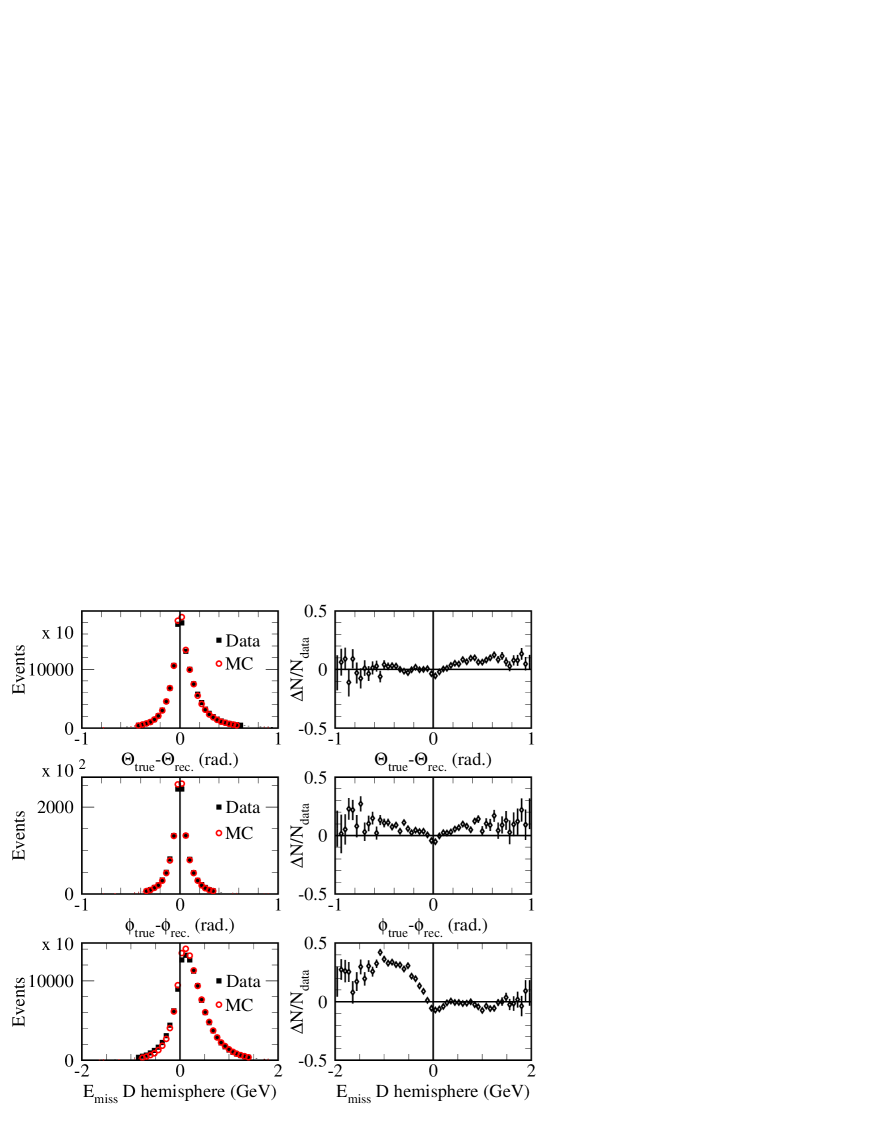
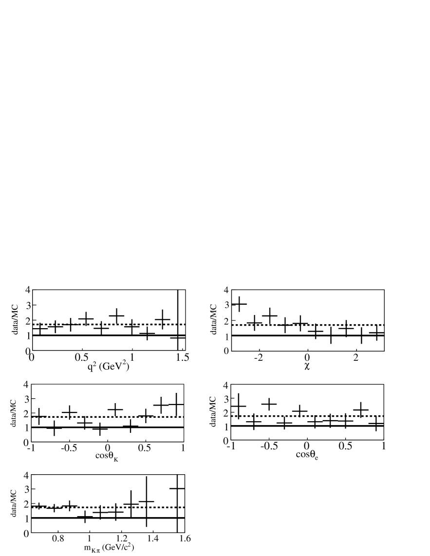
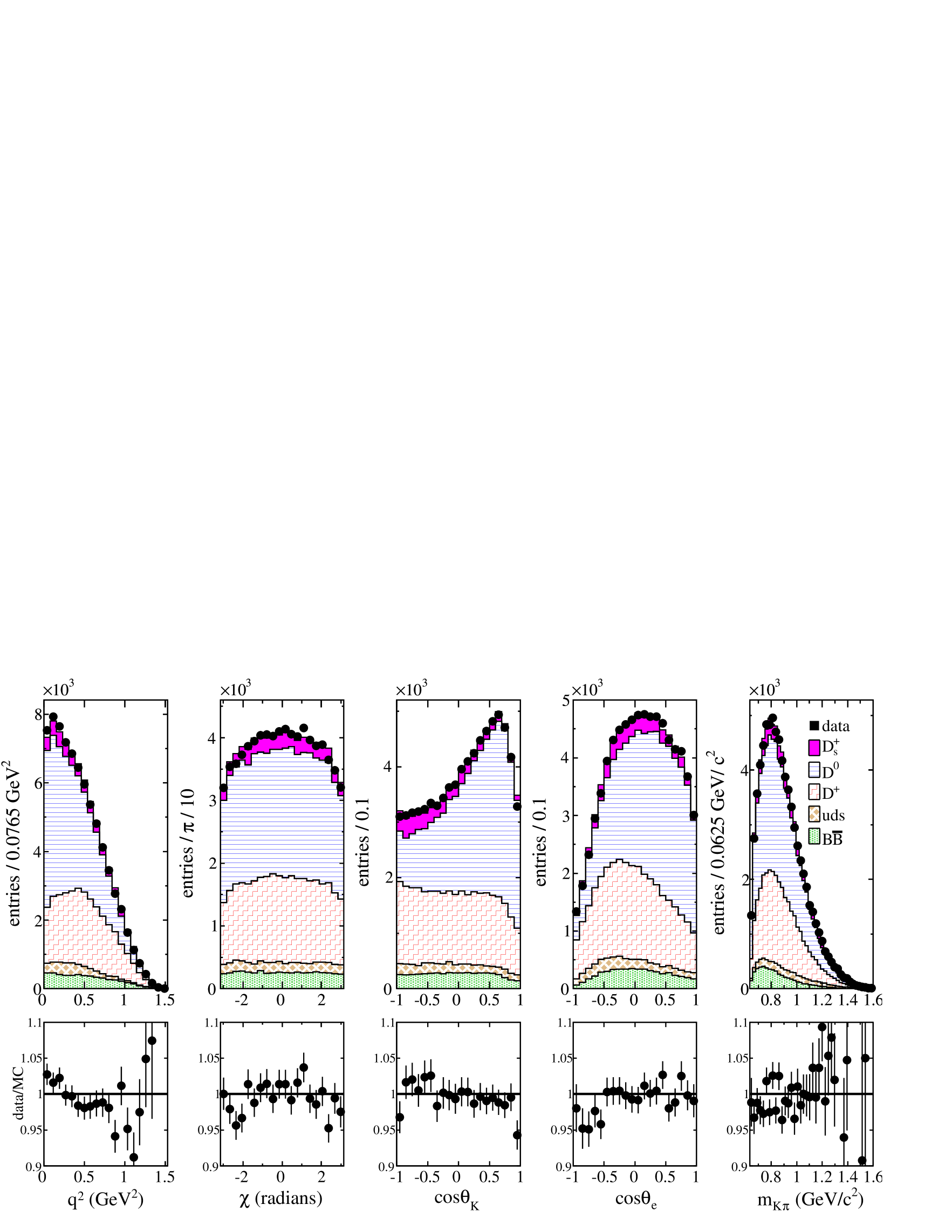
The mass-constrained fit also requires estimates of the uncertainties on the angles defining the $D^{+}$ direction and on the missing energy must also be provided. These estimates are parameterized versus the missing energy in the opposite hemisphere which is used to quantify the quality of the reconstruction in a given event. Parameterizations of these uncertainties are obtained in data and in simulation using events with a reconstructed $D^{+}\rightarrow K^{-}\pi^{+}\pi^{+}$ , for which we can compare the measured $D^{+}$ direction with its estimate using the algorithm employed for the analyzed semileptonic decay channel. $D^{+}\rightarrow K^{-}\pi^{+}\pi^{+}$ events also allow one to control the missing energy estimate and its uncertainty. Corresponding distributions obtained in data and with simulated events are given in Fig. 4. These distributions are similar, and the remaining differences are corrected as explained in Section VI.3.2.

Typical values for the reconstruction accuracy of kinematic variables, obtained by fitting the sum of two Gaussian distributions for each variable, are given in Table 6. These values are only indicative as the matching of reconstructed-to-generated kinematic variables of events in five dimensions is included, event-by-event, in the fitting procedure.

Table 6: Expected resolutions for the five variables. They are obtained by fitting the distributions to the sum of two Gaussian functions. The fraction of events fitted in the broad component is given in the last column.

variable	$\sigma_{1}$	$\sigma_{2}$	fraction of events
			in broadest Gaussian
$\cos\theta_{e}$	0.068	0.325	0.139
$\cos\theta_{K}$	0.145	0.5	0.135
$\chi~(\rm\,rad)$	0.223	1.174	0.135
$q^{2}~(\mathrm{\,Ge\kern-1.00006ptV}^{2})$	0.081	0.264	0.205
$m_{K\pi}~({\mathrm{\,Ge\kern-1.00006ptV\!/}c^{2}})$	0.0027	0.010	0.032

VI.2 Background rejection

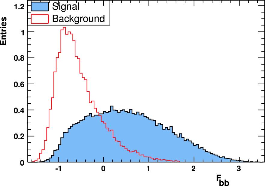
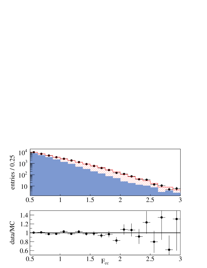
Background events arise from $\mathchar 28935\relax{(4S)}$ decays and hadronic events from the continuum. Three variables are used to decrease the contribution from $B\overline{B}$ events: $R_{2}$ , the total charged and neutral multiplicity, and the sphericity of the system of particles produced in the event hemisphere opposite to the candidate. These variables use topological differences between events with $B$ decays and events with $c\bar{c}$ fragmentation. The particle distribution in $\mathchar 28935\relax{(4S)}$ decay events tends to be isotropic as the $B$ mesons are heavy and produced near threshold, while the distribution in $c\bar{c}$ events is jet-like as the CM energy is well above the charm threshold. These variables are combined linearly in a Fisher discriminant ref:fisher , $F_{bb}$ , and corresponding distributions are given in Fig. 5. The requirement $F_{bb}>0$ retains $70\%$ of signal and 15 $\%$ of $B\overline{B}$ -background events.

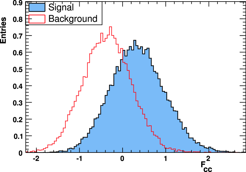
Background events from the continuum arise mainly from charm particles, as requiring an electron and a kaon reduces the contribution from light-quark flavors to a low level. Because charm hadrons take a large fraction of the charm quark energy, charm decay products have higher average energies and different angular distributions (relative to the thrust axis or to the $D$ direction) as compared to other particles in the hemisphere, emitted from the hadronization of the $c$ and $\overline{c}$ quarks. The $D^{+}$ meson decays also at a measurable distance from the beam interaction point, whereas background event candidates contain usually a pion from fragmentation. Therefore, to decrease the amount of background from fragmentation particles in $c\bar{c}$ events, the following variables are used:

•

the spectator system mass;
•

the momentum of the leading spectator track;
•

a quantity derived from the $\chi^{2}$ probability of the $D^{+}$ mass-constrained fit;
•

a quantity derived from the $\chi^{2}$ vertex fit probability of the $K$ , $\pi$ and $e$ trajectories;
•

the value of the $D^{+}$ momentum after the $D^{+}$ mass-constrained fit;
•

the significance of the flight length of the $D^{+}$ from the beam interaction point until its decay point;
•

the ratio between the significances of the distance of the pion trajectory to the $D^{+}$ decay position and to the beam interaction point.

Several of these variables are transformed such that distributions of resulting (derived) quantities have a bell-like shape. These seven variables are combined linearly into a Fisher discriminant variable ( $F_{cc}$ ) and the corresponding distribution is given in Fig. 6; events are kept for values above 0.5. This selection retains $40\%$ of signal events that were kept by the previous selection requirement on $F_{bb}$ and rejects $94\%$ of the remaining background. About $244\times 10^{3}$ signal events are selected with a ratio $S/B=2.3$ . In the mass region of the $\overline{K}^{*}(892)^{0}$ this ratio increases to 4.6. The average efficiency for signal is $2.9\%$ and is uniform when projected onto individual kinematic variables. A loss of efficiency, induced mainly by the requirement of a minimal energy for the positron, is observed for negative values of $\cos{\theta_{e}}$ and at low $q^{2}$ .

VI.3 Simulation tuning

Several event samples are used to correct differences between data and simulation. For the remaining $\mathchar 28935\relax{(4S)}$ decays, the simulation is compared to data as explained in Section VI.3.1. For $e^{+}e^{-}\rightarrow c\overline{c}$ events, corrections to the signal sample are different from those to the background sample. For signal, events with a reconstructed $D^{+}\rightarrow K^{-}\pi^{+}\pi^{+}$ in data and MC are used. These samples allow us to compare the different distributions of the quantities entering in the definition of the $F_{bb}$ and $F_{cc}$ discriminant variables. Measured differences are then corrected, as explained below (Section VI.3.2). These samples are used also to measure the reconstruction accuracy on the direction and missing energy estimates for $D^{+}\rightarrow K^{-}\pi^{+}e^{+}\nu_{e}$ . For background events (Section VI.3.3), the control of the simulation has to be extended to $D^{0}$ , $D^{*+}$ and $D^{+}_{s}$ production and to their accompanying charged mesons. Additional samples with a reconstructed exclusive decay of the corresponding charm mesons are used. Corrections are applied also on the semileptonic decay models such that they agree with recent measurements. Effects of these corrections are verified using wrong sign events (Section VI.3.4), which are used also to correct for the production fractions of charged and neutral $D$ -mesons. Finally, absolute mass measurement capabilities of the detector and the mass resolution are verified (Section VI.3.5) using $D^{0}\rightarrow K^{-}\pi^{+}$ and $D^{+}\rightarrow K^{-}\pi^{+}\pi^{+}$ decay channels.

VI.3.1 Background from $\mathchar 28935\relax{(4S)}$ decays

The distribution of a given variable for events from the remaining $\mathchar 28935\relax{(4S)}\rightarrow B\kern 1.79993pt\overline{\kern-1.79993ptB}{}$ background is obtained by comparing corresponding distributions for events registered at the $\mathchar 28935\relax{(4S)}$ resonance and 40 $\mathrm{\,Me\kern-1.00006ptV}$ below. Compared with expectations from simulated events in Fig. 7, distributions versus the kinematic variables agree reasonably well in shape, within statistics, but the simulation needs to be scaled by $1.7\pm 0.2$ . A similar effect was measured also in a previous analysis of the $D^{+}_{s}\rightarrow K^{-}K^{+}e^{+}\nu_{e}$ decay channel ref:kkenu .

VI.3.2 Simulation tuning of signal events

Events with a reconstructed $D^{+}\rightarrow K^{-}\pi^{+}\pi^{+}$ candidate are used to correct the simulation of several quantities which contribute to the $K^{-}\pi^{+}e^{+}\nu_{e}$ event reconstruction.

Using the $K^{-}\pi^{+}\pi^{+}$ mass distribution, a signal region, between 1.849 and 1.889 ${\mathrm{\,Ge\kern-1.00006ptV\!/}c^{2}}$ , and two sidebands ( $[1.798,~1.838]~{\rm and}~[1.900,~1.940]~{\mathrm{\,Ge\kern-1.00006ptV\!/}c^{2}}$ ), are defined. A distribution of a given variable is obtained by subtracting from the corresponding distribution of events in the signal region half the content of those from sidebands. This approach is referred to as sideband subtraction in the following. It is verified with simulated events that distributions obtained in this way agree with those expected from true signal events.

control of the $c\rightarrow D^{+}$ production mechanism:

the Fisher discriminants $F_{bb}$ and $F_{cc}$ are functions of several variables, listed in Section VI.2, which have distributions that may differ between data and simulation. For a given variable, weights are computed from the ratio of normalized distributions measured in data and simulation. This procedure is repeated, iteratively, considering the various variables, until corresponding projected distributions are similar to those obtained in data. There are remaining differences between data and simulation coming from correlations between variables. To minimize their contribution, the energy spectrum of $D^{+}\rightarrow K^{-}\pi^{+}\pi^{+}$ is weighted in data and simulation to be similar to the spectrum of semileptonic signal events.

We have performed another determination of the corrections without requiring that these two energy spectra are similar. Differences between the fitted parameters obtained using the two sets of corrections are taken as systematic uncertainties.

control of the $D^{+}$ direction and missing energy measurements:

the direction of a fully reconstructed $D^{+}\rightarrow K^{-}\pi^{+}\pi^{+}$ decay is accurately measured and one can therefore compare the values of the two angles, defining its direction, with those obtained when using all particles present in the event except those attributed to the decay signal candidate. The latter procedure is used to estimate of the $D^{+}$ direction for the decay $D^{+}\rightarrow K^{-}\pi^{+}e^{+}\nu_{e}$ . Distributions of the difference between angles measured with the two methods give the corresponding angular resolutions. This event sample allows also one to compare the missing energy measured in the $D^{+}$ hemisphere and in the opposite hemisphere for data and simulated events. These estimates for the $D^{+}$ direction and momentum, and their corresponding uncertainties are used in a mass-constrained fit.

For this study, differences between data and simulation in the $c\rightarrow D^{+}$ fragmentation characteristics are corrected as explained in the previous paragraph. Global cuts similar to those applied for the $D^{+}\rightarrow K^{-}\pi^{+}e^{+}\nu_{e}$ analysis are used such that the topology of $D^{+}\rightarrow K^{-}\pi^{+}\pi^{+}$ selected events is as close as possible to that of semileptonic events. Comparisons between angular resolutions measured in data and simulation indicate that the ratio data/MC is 1.1 in the tails of the distributions (Fig. 4). Corresponding distributions for the missing energy measured in the signal hemisphere ( $E^{same}_{miss.}$ ), in data and simulation, show that these distributions have an offset of about 100 ${\mathrm{\,Me\kern-1.00006ptV\!/}c^{2}}$ (Fig. 4) which corresponds to energy escaping detection even in absence of neutrinos. To evaluate the neutrino energy in $D^{+}$ semileptonic decays this bias is corrected on average.

The difference between the exact and estimated values of the two angles and missing energy is measured versus the value of the missing energy in the opposite event hemisphere ( $E_{miss.}^{opp.}$ ). This last quantity provides an estimate of the quality of the energy reconstruction for a given event. In each slice of $E_{miss.}^{opp.}$ , a Gaussian distribution is fitted and corresponding values of the average and standard deviation are measured. As expected, the resolution gets worse when $E_{miss.}^{opp.}$ increases. These values are used as estimates for the bias and resolution for the considered variable. Fitted uncertainties are slightly higher in data than in the simulation. From these measurements, a correction and a smearing are defined as a function of $E_{miss.}^{opp.}$ . They are applied to simulated event estimates of $\theta,~\phi$ and $E_{miss.}^{same}$ . This additional smearing is very small for the $D^{+}$ direction determination and is typically $\simeq 100~\mathrm{\,Me\kern-1.00006ptV}$ on the missing energy estimate.

After applying corrections, the resolution on simulated events becomes slightly worse than in data. When evaluating systematic uncertainties we have used the total deviation of fitted parameters obtained when applying or not applying the corrections.

VI.3.3 Simulation tuning of charm background events from continuum

As the main source of background originates from track combinations in which particles are from a charm meson decay, and others from hadronization, it is necessary to verify that the fragmentation of a charm quark into a charm meson and that the production characteristics of charged particles accompanying the charm meson are similar in data and in simulation.

In addition, most background events contain a lepton from a charm hadron semileptonic decay. The simulation of these decays is done using the ISGW2 model ref:isgw2 , which does not agree with recent measurements ref:kenu , therefore all simulated decay distributions are corrected.

Corrections on charm quark hadronization:

for this purpose, distributions obtained in data and MC are compared. We study the event shape variables that enter in the Fisher discriminant $F_{bb}$ and for variables entering into $F_{cc}$ , apart from $\chi^{2}$ probability of the mass-constrained fit which is peculiar to the analyzed $D^{+}$ semileptonic decay channel. Production characteristics of charged pions and kaons emitted during the charm quark fragmentation, are also measured, and their rate, momentum, and angle distribution relative to the simulated $D$ direction are corrected. These corrections are obtained separately for particles having the same or the opposite charge relative to the charm quark forming the $D$ hadron. Corrections consist of a weight applied to each simulated event. This weight is obtained iteratively, correcting in turn each of the considered distributions. Measurements are done for $D^{*+}$ , $D^{0}$ (vetoing $D^{0}$ from $D^{*+}$ decays) and for $D^{+}$ . For $D_{s}^{+}$ mesons, only the corresponding $c$ -quark fragmentation distribution is corrected.

Correction of D semileptonic decay form factors:

by default, $D$ semileptonic decays are generated in EvtGen ref:evtgen using the ISGW2 decay model which does not reproduce present measurements (this was shown for instance in the BABAR analysis of $D^{*+}\rightarrow D^{0}\pi^{+},D^{0}\rightarrow K^{-}e^{+}\nu_{e}$ ref:kenu ). Events are weighted such that they correspond to hadronic form factors behaving according to the single pole parameterization as in Eq. (24).

For decay processes of the type $D\rightarrow Pe\nu_{e}$ , where $P$ is a pseudoscalar meson, the weight is proportional to the square of the ratio between the corresponding hadronic form factors, and the total decay branching fraction remains unchanged after the transformation. For all Cabibbo-favored decays a pole mass value equal to $1.893~{\mathrm{\,Ge\kern-1.00006ptV\!/}c^{2}}$ ref:kenu is used whereas for Cabibbo-suppressed decays $1.9~{\mathrm{\,Ge\kern-1.00006ptV\!/}c^{2}}$ ref:cleo_pienu is taken. This value of the pole mass is used also for $D_{s}$ semileptonic decays into a pseudoscalar meson. For decay processes of the type $D\rightarrow Ve\nu_{e},~(V\rightarrow P_{1}P_{2})$ , where $P$ and $V$ are respectively pseudoscalar and vector mesons, corrections depend on the mass of the hadronic system, and on $q^{2},~\cos\theta_{e},~\cos\theta_{K}$ and $\chi$ . They are evaluated iteratively using projections of the differential decay rate versus these variables, as obtained in EvtGen and in a simulation which contains the expected distribution. To account for correlations between these variables, once distributions agree in projection, binned distributions over the five dimensional space are compared and a weight is measured in each bin. For Cabibbo-allowed decays, events are distributed over 2800 bins, similar to those defined in Section VI.4; 243 bins are used for Cabibbo-suppressed decays. Apart for the resonance mass and width which are different for each decay channel, the same values, given in Table 7, are used for the other parameters which determine the differential decay rate.

For decay channels $D\rightarrow K\pi e^{+}\nu_{e}$ an $S$ -wave component is added with the same characteristics as in the present measurements. Other decay channels included in EvtGen ref:evtgen and contributing to this same final state, such as a constant amplitude and the $\overline{K}^{*}_{2}(1430)^{0}$ components, are removed as they are not observed in data.

All branching fractions used in the simulation agree within uncertainties with the current measurements ref:pdg10 (apart for $D\rightarrow\pi e^{+}\nu_{e}$ , which is then rescaled). Only the shapes of charm semileptonic decay distributions are corrected.

Systematic uncertainties related to these corrections are estimated by varying separately each parameter according to its expected uncertainty, given in Table 7.

Table 7: Central values and variation range for the various parameters which determine the differential decay rate in

D\rightarrow P/Ve^{+}\nu_{e}

decays, used to correct the simulation and to evaluate corresponding systematic uncertainties. The form factors

A_{1}(q^{2}),~A_{2}(q^{2})~{\rm and}~V(q^{2})

and the mass parameters

m_{A}

and

m_{V}

are defined in Eq. (24).

parameter	central	variation
	value	interval
$m_{pole}(D^{0,+}\rightarrow Ke^{+}\nu_{e})$	$1.893~{\mathrm{\,Ge\kern-1.00006ptV\!/}c^{2}}$	$\pm 30~{\mathrm{\,Me\kern-1.00006ptV\!/}c^{2}}$
$m_{pole}(D^{0,+}\rightarrow\pi e^{+}\nu_{e})$	$1.9~{\mathrm{\,Ge\kern-1.00006ptV\!/}c^{2}}$	$\pm 100~{\mathrm{\,Me\kern-1.00006ptV\!/}c^{2}}$
$m_{pole}(D_{s}^{+}\rightarrow\eta/\eta^{\prime}e^{+}\nu_{e})$	$1.9~{\mathrm{\,Ge\kern-1.00006ptV\!/}c^{2}}$	$\pm 100~{\mathrm{\,Me\kern-1.00006ptV\!/}c^{2}}$
$r_{2}=\|A_{2}(0)\|/\|A_{1}(0)\|$	$0.80$	$\pm 0.05$
$r_{V}=\|V(0)\|/\|A_{1}(0)\|$	$1.50$	$\pm 0.05$
$m_{A}$	$2.5~{\mathrm{\,Ge\kern-1.00006ptV\!/}c^{2}}$	$\pm 0.3~{\mathrm{\,Ge\kern-1.00006ptV\!/}c^{2}}$
$m_{V}$	$2.1~{\mathrm{\,Ge\kern-1.00006ptV\!/}c^{2}}$	$\pm 0.2~{\mathrm{\,Ge\kern-1.00006ptV\!/}c^{2}}$
$r_{BW}$	$3.0~({\mathrm{\,Ge\kern-1.00006ptV\!/}c})^{-1}$	$\pm 0.3~({\mathrm{\,Ge\kern-1.00006ptV\!/}c}^{-1})$

VI.3.4 Wrong sign event analysis

Wrong-sign (WS) events of the type $K^{-}\pi^{-}e^{+}$ are used to verify if corrections applied to the simulation improve the agreement with data, because the origin of these events is quite similar to that of the background contributing in right-sign $K^{-}\pi^{+}e^{+}$ (RS) events. The ratio between the measured and expected number of WS events is $0.950\pm 0.005$ . In RS events the number of background candidates is a free parameter in the fit.

At this point corrections have been evaluated separately for charged and neutral $D$ mesons. As the two charged states correspond to background distributions having different shapes, it is also possible to correct for their relative contributions. We improve the agreement with data by increasing the fraction of events with a $D^{0}$ meson in MC by 4 $\%$ and correspondingly decreasing the fraction of $D^{+}$ by $5\%$ . After corrections, projected distributions of the five kinematic variables obtained in data and simulation are given in Fig. 8.

VI.3.5 Absolute mass scale.

The absolute mass measurement is verified using exclusive reconstruction of charm mesons in data and simulation. For candidate events $D^{*+}\rightarrow D^{0}\pi^{+},~D^{0}\rightarrow K^{-}\pi^{+}$ , the mean and RMS values of the $D^{0}$ mass distribution are measured from a fit of the sum to a Gaussian distribution for the signal and a first order polynomial for the background. The $D^{0}$ mass reconstructed in simulation is very close to expectation, $\Delta_{m}^{MC}=(-0.07\pm 0.01)~{\mathrm{\,Me\kern-1.00006ptV\!/}c^{2}}$ , whereas in data it differs by $\Delta_{m}^{data}=(-1.07\pm 0.17)~{\mathrm{\,Me\kern-1.00006ptV\!/}c^{2}}$ . Here $\Delta_{m}$ is the difference between the reconstructed and the exact or the world average mass values when analyzing MC or data respectively. The uncertainty quoted for $\Delta_{m}^{data}$ is from Ref. ref:pdg10 . To correct for this effect the momentum ( $p$ ) of each track in data, measured in the laboratory frame, is increased by an amount: $\Delta_{p}^{data}=0.7\times 10^{-3}p$ . The standard deviation of the Gaussian fitted on the $D^{0}$ signal is slightly smaller in simulation, $(7.25\pm 0.01)~{\mathrm{\,Me\kern-1.00006ptV\!/}c^{2}}$ , than in data, $(7.39\pm 0.01)~{\mathrm{\,Me\kern-1.00006ptV\!/}c^{2}}$ . The difference between the widths of reconstructed $D^{0}$ signals in the two samples, is measured versus the transverse momentum of the tracks emitted in the decay. In simulation, the measured transverse momenta of the tracks are smeared to correct for this difference.

Having applied these corrections, $D^{+}$ mass distributions, for the decay $D^{+}\rightarrow K^{-}\pi^{+}\pi^{+}$ obtained in data and simulation are compared. The standard deviation of the fitted Gaussian distribution on signal is now similar in data and simulation. The reconstructed $D^{+}$ mass is higher by $0.23~{\mathrm{\,Me\kern-1.00006ptV\!/}c^{2}}$ in simulation (on which no correction was applied) and by $0.32~{\mathrm{\,Me\kern-1.00006ptV\!/}c^{2}}$ in data. These remaining differences are not corrected and included as uncertainties.

VI.4 Fitting procedure

A binned distribution of data events is analyzed. The expected number of events in each bin depends on signal and background estimates and the former is a function of the values of the fitted parameters.

We perform a minimization of a negative log-likelihood distribution. This distribution has two parts. One corresponds to the comparison between measured and expected number of events in bins which span the five dimensional space of the differential decay rate. The other part uses the distribution of the values of the Fisher discriminant variable $F_{cc}$ to measure the fraction of background events.

There are respectively 5, 5 and 4 equal size bins for the variables $\chi$ , $\cos\theta_{K}$ and $\cos\theta_{e}$ . For $q^{2}$ and $m_{K\pi}$ we use respectively 4 and 7 bins of different size such that they contain approximately the same number of signal events. There are 2800 bins ( $N_{\mathrm{bins}}$ ) in total.

The likelihood expression is:

$\displaystyle{\cal L}$	$\displaystyle=$	$\displaystyle\prod^{N_{\mathrm{bins}}}_{i=0}{P(n^{i}_{\mathrm{data}}\|n^{i}_{\mathrm{MC}})}$	(34)
	$\displaystyle\times$	$\displaystyle\prod^{N_{\mathrm{data}}}_{j=1}\left[\frac{N_{\mathrm{sig}}}{N_{\mathrm{sig}}+N_{\mathrm{bkg}}}\times pdf_{\mathrm{sig}}^{j}\right.$
	$\displaystyle+$	$\displaystyle\left.\frac{N_{\mathrm{bkg}}}{N_{\mathrm{sig}}+N_{\mathrm{bkg}}}\times{pdf_{\mathrm{bkg}}^{j}}\right],$

where $n_{\mathrm{data}}^{i}$ is the number of data events in bin $i$ and $n_{\mathrm{MC}}^{i}$ is the sum of MC estimates for signal and background events in the same bin. $P(n^{i}_{\mathrm{data}}|n^{i}_{\mathrm{MC}})$ is the Poisson probability for having $n_{\mathrm{data}}^{i}$ events in bin $i$ where $n_{\mathrm{MC}}^{i}$ events are expected, on average, where:

$\displaystyle n_{\mathrm{MC}}^{i}$	$\displaystyle=$	$\displaystyle\sum^{N_{\mathrm{events}}^{\mathrm{bin}~i}}_{j=0}\left[\frac{N_{\mathrm{sig}}}{W_{\mathrm{fit}}^{\mathrm{tot}}(\vec{\lambda_{0}},\vec{\lambda})}\frac{W_{j}(\vec{\lambda})}{W_{j}(\vec{\lambda_{0}})}C_{j}\right]$	(35)
	$\displaystyle+$	$\displaystyle\frac{N_{\mathrm{bkg}}}{W_{\mathrm{bkg}}^{\mathrm{tot}}}\times{W_{\mathrm{bkg}}^{i}};$	(35)
$\displaystyle W^{\mathrm{tot}}_{\mathrm{fit}}(\vec{\lambda_{0}},\vec{\lambda})$	$\displaystyle=$	$\displaystyle\sum^{N_{\mathrm{events}}^{\mathrm{all~bins}}}_{j=0}\frac{W_{j}(\vec{\lambda})}{W_{j}(\vec{\lambda_{0}})}C_{j}.$

The summation to determine $n_{\mathrm{MC}}^{i}$ extends over all generated signal events which are reconstructed in bin $i$ . The terms $\vec{\lambda}~{\rm and}~\vec{\lambda_{0}}$ are, respectively, the values of parameters used in the fit and those used to produce simulated events. $W_{j}(\vec{\lambda})$ is the value of the expression for the decay rate (see Eq. (16)) for event $j$ using the set of parameters $(\vec{\lambda})$ . In these expressions, generated values of the kinematic variables are used. $C_{j}$ is the weight applied to each signal event to correct for differences between data and simulation. It is left unchanged during the fit. $W_{\mathrm{bkg}}^{i}$ is the estimated number of background events in bin $i$ given by the simulation, corrected for measured differences with data, as explained in Section VI.3. $W_{\mathrm{bkg}}^{\mathrm{tot}}$ is the estimated total number of background events.

$N_{\mathrm{sig}}$ and $N_{\mathrm{bkg}}$ are respectively the total number of signal and background events fitted in the data sample which contains $N_{\mathrm{data}}$ events. $pdf_{\mathrm{sig}}^{j}$ and $pdf_{\mathrm{bkg}}^{j}$ are the probability density functions for signal and background, respectively, evaluated at the value of the $F_{cc}$ variable for event $j$ . The following expressions are used :

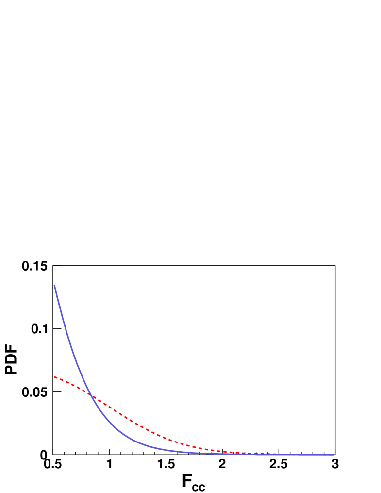
$\displaystyle\displaystyle pdf_{\mathrm{sig}}(F_{cc})$	$\displaystyle=$	$\displaystyle{\cal N}_{\mathrm{sig}}\left\{c_{2}\times\exp\left[\frac{-(F_{cc}-c_{0})^{2}}{2c_{1}^{2}}\right]\right.$
	$\displaystyle+$	$\displaystyle\left.c_{5}\times\exp\left[\frac{-(F_{cc}-c_{3})^{2}}{2c_{4}^{2}}\right]\right\},$
$\displaystyle pdf_{\mathrm{bkg}}(F_{cc})$	$\displaystyle=$	$\displaystyle{\cal N}_{\mathrm{bkg}}\left\{\exp\left[\sum_{i=0}^{4}d_{i}(F_{cc})^{i}\right]\right\}$	(36)

and values of the corresponding parameters $c_{0-5}$ and $d_{0-4}$ are determined from fits to binned distributions of $F_{cc}$ in simulated signal and background samples. ${\cal N}_{\mathrm{sig}}$ and ${\cal N}_{\mathrm{bkg}}$ are normalization factors. In Fig. 9 these two distributions are drawn to illustrate their different behavior versus the values of $F_{cc}$ for signal and background events. As expected, the $pdf_{\mathrm{bkg}}$ distribution has higher values at low $F_{cc}$ than the corresponding distribution for signal.

VI.4.1 Background smoothing

As the statistics of simulated background events for the charm continuum is only $1.6$ times the data, biases appear in the determination of the fit parameters if we use simply, as estimates for background in each bin, the actual values obtained from the MC. Using a parameterized event generator, this effect is measured using distributions of the difference between the fitted and exact values of a parameter divided by its fitted uncertainty (pull distributions). To reduce these biases, a smoothing ref:Cranmer of the background distribution is performed. It consists of distributing the contribution of each event, in each dimension, according to a Gaussian distribution. In this procedure correlations between variables are neglected. To account for boundary effects, the dataset is reflected about each boundary. $\chi$ is essentially uncorrelated with all other variables and in particular with $\cos\theta_{l}$ . Therefore, for each bin in ( $m,~q^{2}~{\rm and}~\cos\theta_{K}$ ), a smoothing of the $\chi$ and $\cos\theta_{l}$ distributions is done in the hypothesis that these two variables are independent.

VII $D^{+}\rightarrow\overline{K}^{*0}e^{+}\nu_{e}$ hadronic form factor measurements

We first consider a signal made of the $\overline{K}^{*}(892)^{0}$ and $S$ -wave components. Using the LASS parameterization of the $S$ -wave phase versus the $K\pi$ mass (Eq. (10)), values of the following quantities (quoted in Table 8 second column) are obtained from a fit to data :

•

parameters of the $K^{*}(892)^{0}$ Breit-Wigner distribution: $m_{K^{*}(892)}$ , $\Gamma^{0}_{K^{*}(892)}$ , and $r_{BW}$ , the Blatt-Weisskopf parameter;
•

parameters of the $D^{+}\rightarrow\overline{K}^{*0}e^{+}\nu_{e}$ hadronic form factors: $r_{2},~r_{V}$ , and $m_{A}$ . The parameter $m_{V}$ which determines the $q^{2}$ variation of the vector form factor is fixed to $2.0~{\mathrm{\,Ge\kern-1.00006ptV\!/}c^{2}}$ ;
•

parameters which define the $S$ -wave component: $r_{S}$ and $r_{S}^{(1)}$ for the amplitude (Eq. (28)), $a_{S,BG}^{1/2}$ and $b_{S,BG}^{1/2}$ for the phase (Eq. (8));
•

and finally the total numbers of signal and background events, $N_{sig}$ and $N_{bkg}$ .

Table 8: Values of fitted parameters assuming that the final state consists of a sum of

S

-wave and

\overline{K}^{*}(892)^{0}

components (second column), includes the

\overline{K}^{*}(1410)^{0}

in the

P

-wave (third column) and a

D

-wave (last column). The variation of the

S

-wave phase versus the

K\pi

mass is parameterized according to Eq. (10) whereas the

S

-wave amplitude is parameterized as in Eq. (28). Fit results including the

\overline{K}^{*}(1410)^{0}

are discussed in Section VIII.1. Values given in the third column of this Table are the central results of this analysis.

variable	$S+\overline{K}^{*}(892)^{0}$	$S+\overline{K}^{*}(892)^{0}$	$S+\overline{K}^{*}(892)^{0}$
		$\overline{K}^{*}(1410)^{0}$	$\overline{K}^{*}(1410)^{0}+D$
$m_{K^{*}(892)}({\mathrm{\,Me\kern-1.00006ptV\!/}c^{2}})$	$894.77\pm{0.08}$	$895.43\pm{0.21}$	$895.27\pm{0.15}$
$\Gamma^{0}_{K^{*}(892)}({\mathrm{\,Me\kern-1.00006ptV\!/}c^{2}})$	$45.78\pm{0.23}$	$46.48\pm{0.31}$	$46.38\pm{0.26}$
$r_{BW}({\mathrm{\,Ge\kern-1.00006ptV\!/}c})^{-1}$	$3.71\pm{0.22}$	$2.13\pm{0.48}$	$2.31\pm{0.20}$
$m_{A}({\mathrm{\,Ge\kern-1.00006ptV\!/}c^{2}})$	$2.65\pm 0.10$	$2.63\pm 0.10$	$2.58\pm 0.09$
$r_{V}$	$1.458\pm{0.016}$	$1.463\pm{0.017}$	$1.471\pm{0.016}$
$r_{2}$	$0.804\pm{0.020}$	$0.801\pm{0.020}$	$0.786\pm{0.020}$
$r_{S}(\mathrm{\,Ge\kern-1.00006ptV})^{-1}$	$-0.470\pm{0.032}$	$-0.497\pm{0.029}$	$-0.548\pm{0.027}$
$r^{(1)}_{S}$	$0.17\pm{0.08}$	$0.14\pm{0.06}$	$0.03\pm{0.06}$
$a_{S,BG}^{1/2}({\mathrm{\,Ge\kern-1.00006ptV\!/}c})^{-1}$	$1.82\pm{0.14}$	$2.18\pm{0.14}$	$2.10\pm{0.10}$
$b_{S,BG}^{1/2}({\mathrm{\,Ge\kern-1.00006ptV\!/}c})^{-1}$	$-1.66\pm{0.65}$	$1.76$ fixed	$1.76$ fixed
$r_{K^{*}(1410)^{0}}$		$0.074\pm{0.016}$	$0.052\pm{0.013}$
$\delta_{K^{*}(1410)^{0}}({\rm degree})$		$8.3\pm{13.0}$	$0$ fixed
$r_{D}(\mathrm{\,Ge\kern-1.00006ptV})^{-4}$			$0.78\pm 0.18$
$\delta_{D}({\rm degree})$			$0$ fixed
$N_{sig}$	$243850\pm{699}$	$243219\pm{713}$	$243521\pm{688}$
$N_{bkg}$	$107370\pm{593}$	$108001\pm{613}$	$107699\pm{583}$
Fit probability	$4.6\%$	$6.4\%$	$8.8\%$

Apart from the effective range parameter, $b_{S,BG}^{1/2}$ , all other quantities are accurately measured. Values for the $S$ -wave parameters depend on the parameterization used for the $P$ -wave and as the LASS experiment includes a $K^{*}(1410)$ and other components one cannot directly compare our results on $a_{S,BG}^{1/2}$ and $b_{S,BG}^{1/2}$ with those of LASS. We have obtained the first measurement for $m_{A}$ which gives the $q^{2}$ variation of the axial vector hadronic form factors. Using the values of fitted parameters and integrating the corresponding differential decay rates, fractions of $S$ - and $P$ -wave are given in the second column of Table 9.

Table 9: Fractions for signal components assuming that the final state consists of a sum of

S

-wave and

\overline{K}^{*}(892)^{0}

components (second column), including the

\overline{K}^{*}(1410)^{0}

in the

P

-wave (third column) and a

D

-wave (last column). In the second and third cases, the sum of the fractions for the two

\overline{K}^{*}

does not correspond exactly to the total

P

-wave fraction because of interference.

Component	$S+\overline{K}^{*}(892)^{0}$	$S+\overline{K}^{*}(892)^{0}$	$S+\overline{K}^{*}(892)^{0}$
	$(\%)$	$+\overline{K}^{*}(1410)^{0}(\%)$	$\overline{K}^{*}(1410)^{0}+D(\%)$
$S$ -wave	$5.62\pm 0.14\pm 0.13$	$5.79\pm 0.16\pm 0.15$	$5.69\pm 0.16\pm 0.15$
$P$ -wave	$94.38$	$94.21$	$94.12$
$\overline{K}^{*}(892)^{0}$	$94.38$	$94.11\pm 0.74\pm 0.75$	$94.41\pm 0.15\pm 0.20$
$\overline{K}^{*}(1410)^{0}$	$0$	$0.33\pm 0.13\pm 0.19$	$0.16\pm 0.08\pm 0.14$
$D$ -wave	$0$	$0$	$0.19\pm 0.09\pm 0.09$

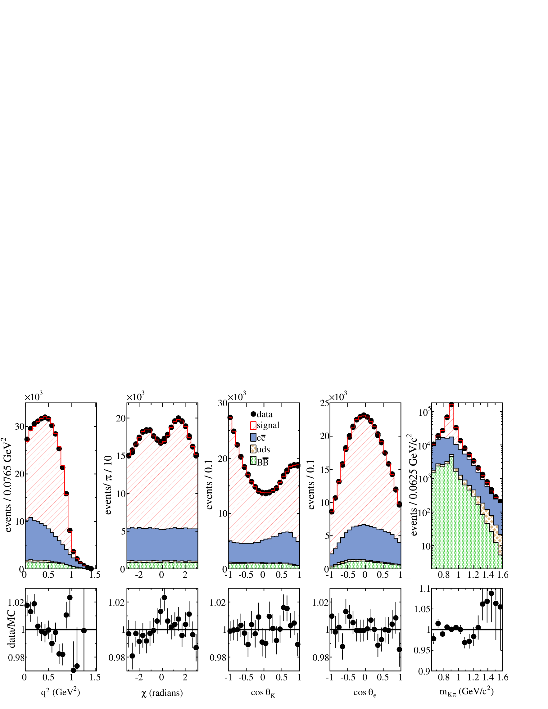
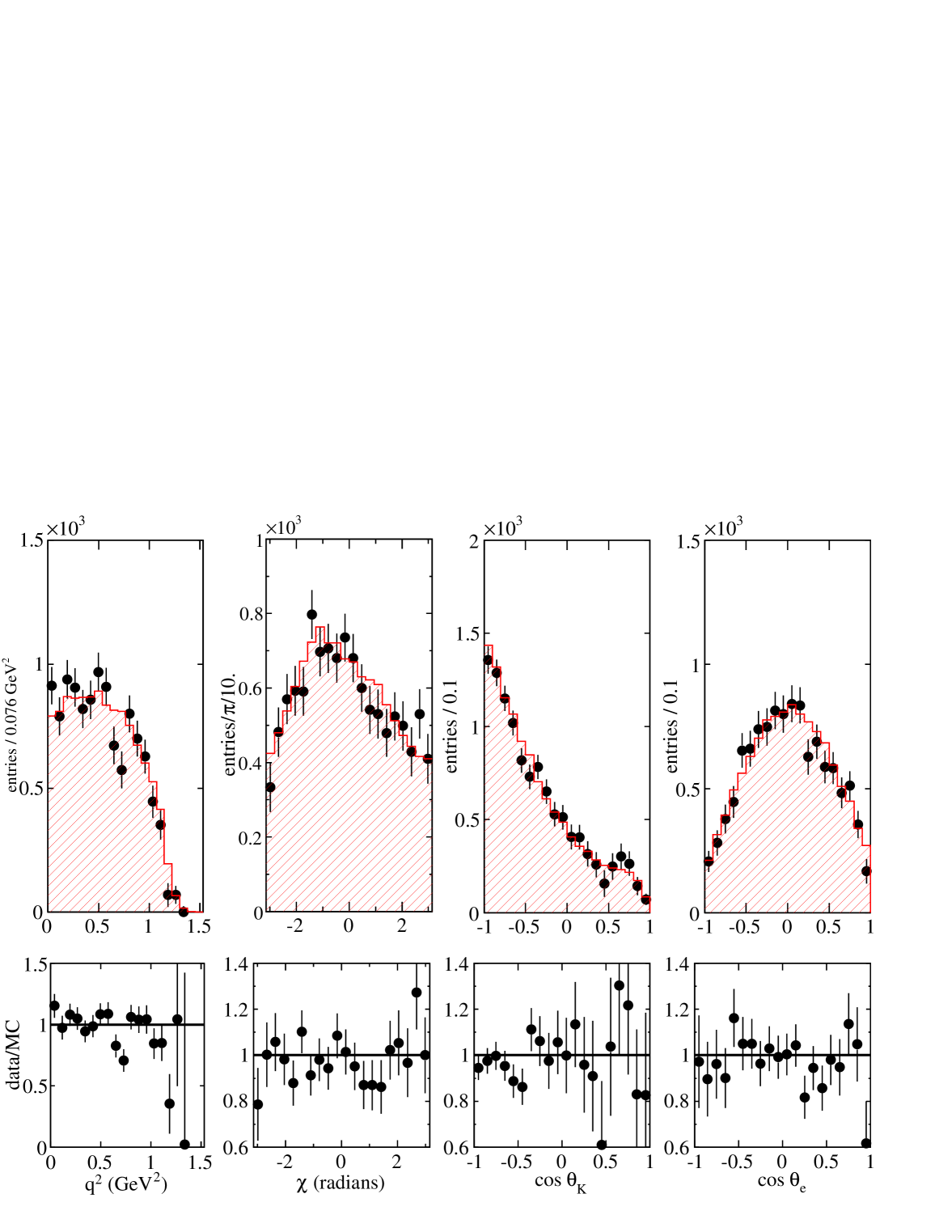
Projected distributions, versus the five variables, obtained in data and from the $S$ -wave + $\overline{K}^{*}(892)^{0}$ fit result are displayed in Fig. 10. The total $\chi^{2}$ of this fit is 2914 for 2787 degrees of freedom which corresponds to the probability of 4.6 $\%$ . Fit results including the $\overline{K}^{*}(1410)^{0}$ and $D$ -wave are discussed in Section VIII.

VII.1 Systematic uncertainties

The systematic uncertainty on each fitted parameter ( $x$ ) is defined as the difference between the fit results in nominal conditions $(x[0])$ and those obtained, $(x[i])$ , after changing a variable or a condition ( $i$ ) by an amount which corresponds to an estimate of the uncertainty in the determination of this quantity:

\displaystyle\Delta x=x[0]-x[i].

(37)

Values are given in Table 10. Some of the corrections induce a variation on the $F_{cc}$ distributions for signal or background which are therefore reevaluated.

VII.1.1 Signal production and decay

Corrections of distributions of Fisher input variables (I):

the signal control sample is corrected as explained in Section VI.3.2. The corresponding systematic uncertainty is obtained by defining new event weights without taking into account that the momentum distribution of reconstructed $D$ mesons is different in hadronic and in semileptonic samples.

Simulation of radiative events (II):

most of radiative events correspond to radiation from the charged lepton, although a non-negligible fraction comes from radiation of the $K^{*}(892)^{0}$ decay products. In $D\rightarrow Pe\nu_{e}$ , by comparing two generators (PHOTOS ref:photos and KLOR ref:klor ), the CLEO-c collaboration has used a variation of $16\%$ to evaluate corresponding systematic uncertainties ref:cleocrad . We have increased the fraction of radiative events (simulated by PHOTOS) by 30 $\%$ (keeping constant the total number of events) and obtained the corresponding variations on fitted parameters.

Table 10: Systematic uncertainties on parameters fitted using the

S

-wave and

\overline{K}^{*}(892)^{0}

model, expressed as

(x[0]-x[i])/\sigma_{stat}

: (I) uncertainty associated with the tuning of the signal control sample, (II) fraction of radiative signal events increased by

30\%

, (III) no PID corrections on electron or kaon in MC signal events, (IV) no smearing applied on

\theta_{D},~\phi_{D}~{\rm and}~E_{miss}

for simulated signal events, (V)

B\overline{B}

background rate lowered by the statistical uncertainty of its determination, (VI) uncertainty associated with the tuning of fragmentation in charm background events, (VII) remaining uncertainty on semileptonic decay models in charm background events, (VIII) uncertainty associated with c-meson relative fractions, (IX) uncertainty remaining from the smoothing of the background distribution, (X) effects from limited statistics in simulation, (XI) variation of parameters that were kept constant in the fit and, (XII) absolute mass scale uncertainties.

variation	$\Delta M_{K^{*}(892)^{0}}$	$\Delta\Gamma_{K^{*}(892)^{0}}$	$\Delta r_{BW}$	$\Delta m_{A}$	$\Delta r_{V}$	$\Delta r_{2}$	$\Delta r_{S}$	$\Delta r^{(1)}_{S}$	$\Delta a_{S,BG}^{1/2}$	$\Delta b_{S,BG}^{1/2}$	$\Delta N_{S}$	$\Delta N_{B}$
signal
I	-0.13	-0.16	-0.10	-0.18	0.28	0.18	-0.40	-0.43	0.02	0.00	-0.36	0.44
II	-0.36	0.07	0.02	-0.11	0.34	0.10	0.26	0.20	0.17	0.21	-0.21	0.26
III	0.21	0.13	0.27	0.69	0.78	0.51	0.17	0.16	0.29	0.17	0.18	0.22
IV	0.29	0.36	0.20	-0.18	0.07	-0.25	0.15	0.19	-0.31	-0.23	0.57	-0.70
$B\overline{B}$ bkg.
V	-0.06	0.32	0.09	0.22	-0.13	0.03	0.30	0.31	0.14	0.30	-0.09	0.11
$c\overline{c}$ bkg.
VI	-0.04	0.21	-0.61	0.10	-0.08	0.07	0.33	0.32	0.13	0.27	0.06	-0.08
VII	0.53	0.19	0.14	0.16	0.13	0.07	0.10	0.10	0.17	0.19	0.16	0.22
VIII	0.24	0.36	0.11	-0.49	0.85	0.04	-0.76	-0.68	-0.77	1.02	0.76	-0.91
Fitting procedure
IX	0.13	0.17	0.25	0.29	0.30	0.25	0.25	0.25	0.32	0.32	0.13	0.13
X	0.70	0.70	0.70	0.70	0.70	0.70	0.70	0.70	0.70	0.70	0.70	0.70
XI	0.00	0.00	0.07	0.07	1.15	0.08	0.05	0.05	1.43	0.46	0.01	0.01
XII	-0.93	-0.06	0.09	0.09	-0.05	0.04	0.03	0.02	0.07	-0.05	0.00	0.00
$\sigma_{syst}$	1.41	1.00	1.06	1.21	1.87	0.97	1.27	1.23	1.87	1.47	1.29	1.48

Particle identification efficiencies (III):

the systematic uncertainty is estimated by not correcting for remaining differences between data and MC on particle identification.

Estimates of the values and uncertainties for the $D$ direction and missing energy (IV):

in Section VI.3.2 it is observed that estimates of the $D^{+}$ direction and energy are more accurate in the simulation than in data. After applying smearing corrections, the result of this comparison is reversed. The corresponding systematic uncertainty is equal to the difference on fitted parameters obtained with and without smearing.

VII.1.2 $B\overline{B}$ background correction (V)

The number of remaining $B\overline{B}$ background events expected from simulation is rescaled by $1.7\pm 0.2$ (see Section VI.3.1). The uncertainty on this quantity is used to evaluate corresponding systematic uncertainties.

VII.1.3 Corrections to the $c\bar{c}$ background

Fragmentation associated systematic uncertainties (VI):

after applying corrections explained in Section VI.3.3, the remaining differences between data and simulation for the considered distributions are five times smaller. Therefore, 20 $\%$ of the full difference measured before applying corrections is used as the systematic uncertainty.

Form-factor correction systematics (VII):

corresponding systematic uncertainties depend on uncertainties on parameters used to model the differential semileptonic decay rate of the various charm mesons (see Section VI.3.3).

Hadronization-associated systematic uncertainties (VIII):

using WS events, it is found in Section VI.3.4 that the agreement between data and simulation improves by changing the hadronization fraction of the different charm mesons. Corresponding variations of relative hadronization fractions are compatible with current experimental uncertainties on these quantities. The corresponding systematic uncertainty is obtained by not applying these corrections.

VII.1.4 Fitting procedure

Background Smoothing (IX):

the MC background distribution is smoothed as explained in Section VI.4.1. The evaluation of the associated systematic uncertainty is performed by measuring with simulations based on parameterized distributions, the dispersion of displacements of the fitted quantities when the smoothing is or is not applied in a given experiment. It is verified that uncertainties on the values of the two parameters used in the smoothing have negligible contributions to the resulting uncertainty.

Limited statistics of simulated events (X):

fluctuations of the number of MC events in each bin are not included in the likelihood expression, therefore one quantifies this effect using fits on distributions obtained with a parameterized event generator. Pull distributions of fitted parameters, obtained in similar conditions as in data, have an RMS of 1.2. This increase is attributed to the limited MC statistics used for the signal (4.5 times the data) and, also, from the available statistics used to evaluate the background from $e^{+}e^{-}\rightarrow c\overline{c}$ continuum events. We have included this effect as a systematic uncertainty corresponding to 0.7 times the quoted statistical uncertainty of the fit. It corresponds to the additional fluctuation needed to obtain a standard deviation of 1.2 of the pull distributions.

VII.1.5 Parameters kept constant in the fit (XI).

The signal model has three fixed parameters, the vector pole mass $m_{V}$ and the mass and width of the $\overline{K}^{*}_{0}(1430)$ resonance. Corresponding systematic uncertainties are obtained by varying the values of these parameters. For $m_{V}$ a $\pm 100~{\mathrm{\,Me\kern-1.00006ptV\!/}c^{2}}$ variation is used, whereas for the other two quantities we take respectively $\pm 50~{\mathrm{\,Me\kern-1.00006ptV\!/}c^{2}}$ and $\pm 80~{\mathrm{\,Me\kern-1.00006ptV\!/}c^{2}}$ ref:pdg10 .

VII.1.6 Absolute mass scale (XII).

When corrections defined in Section VI.3.5 are applied, in data and simulation, for the $D^{+}\rightarrow K^{-}\pi^{+}e^{+}\nu_{e}$ decay channel, the fitted $K^{*}(892)^{0}$ mass in data increases by $0.26~{\mathrm{\,Me\kern-1.00006ptV\!/}c^{2}}$ and its width decreases by $0.12~{\mathrm{\,Me\kern-1.00006ptV\!/}c^{2}}$ . The uncertainty on the absolute mass measurement of the $K^{*}(892)^{0}$ is obtained by noting that a mass variation, $\Delta_{m}^{\mathrm{data}}$ , of the $D$ reference signal is reduced by a factor of four in the $K^{*}$ mass region; this gives:

	$\displaystyle\sigma(m_{K^{*}(892)^{0}})$	$\displaystyle=$	$\displaystyle\sqrt{0.17^{2}+0.23^{2}}\frac{\Delta_{m}^{\mathrm{data}}(K\pi)}{\Delta_{m}^{\mathrm{data}}(D^{0,+})}$		(38)
		$\displaystyle\simeq$	$\displaystyle 0.07~{\mathrm{\,Me\kern-1.00006ptV\!/}c^{2}}.$		(38)

In this expression, $0.17~{\mathrm{\,Me\kern-1.00006ptV\!/}c^{2}}$ is the uncertainty on the $D^{0}$ mass ref:pdg10 and $0.23~{\mathrm{\,Me\kern-1.00006ptV\!/}c^{2}}$ is the difference between the reconstructed and exact values of the $D^{+}$ mass in

Table 11: Systematic uncertainties on parameters fitted using a model for the signal which contains

S

-wave,

\overline{K}^{*}(892)^{0}

and

\overline{K}^{*}(1410)^{0}

components, expressed as

(x[0]-x[i])/\sigma_{stat}

: (I) uncertainty associated with the tuning of the signal control sample, (II) fraction of radiative signal events increased by

30\%

, (III) no PID corrections on electron or kaon in MC signal events, (IV) no smearing applied on

\theta_{D},~\phi_{D}~{\rm and}~E_{miss}

for simulated signal events, (V)

B\overline{B}

background rate lowered by the statistical uncertainty of its determination, (VI) uncertainty associated with the tuning of fragmentation in charm background events, (VII) remaining uncertainty on semileptonic decay models for background events, (VIII) uncertainty associated with c-meson relative fractions, (IX) uncertainty remaining from the smoothing of the background distribution, (X) effects from limited statistics in simulation, (XI) variation of parameters that were kept constant in the fit, (XII) uncertainties on absolute mass scale.

variation	$\Delta M_{K^{*}(892)^{0}}$	$\Delta\Gamma_{K^{*}(892)^{0}}$	$\Delta r_{BW}$	$\Delta m_{A}$	$\Delta r_{V}$	$\Delta r_{2}$	$\Delta r_{S}$	$\Delta r^{(1)}_{S}$	$\Delta a_{S,BG}^{1/2}$	$\Delta r_{K^{*}(1410)^{0}}$	$\Delta\delta_{K^{*}(1410)^{0}}$	$\Delta N_{S}$	$\Delta N_{B}$
signal
(I)	0.17	0.05	-0.23	-0.22	-0.31	0.18	0.14	-0.14	-0.13	0.23	-0.19	-0.39	0.45
(II)	-0.18	0.06	-0.01	-0.14	-0.36	0.09	-0.10	0.08	0.05	-0.08	-0.08	-0.23	0.26
(III)	0.02	0.10	0.06	0.70	0.73	0.53	0.14	0.07	0.41	0.08	0.22	0.10	0.12
(IV)	-0.13	0.03	0.29	-0.18	-0.04	-0.27	-0.02	0.02	-0.17	-0.18	0.32	0.61	-0.70
$B\overline{B}$ bkg.
(V)	-0.41	-0.04	0.34	0.26	0.16	0.05	-0.12	0.12	0.08	-0.46	0.22	-0.01	0.02
$c\overline{c}$ bkg.
(VI)	-0.14	0.07	-0.08	0.13	0.09	0.09	-0.16	0.14	-0.01	-0.24	-0.03	0.08	-0.09
(VII)	0.09	0.08	0.14	0.19	0.14	0.08	0.18	0.15	0.06	0.10	0.11	0.14	0.18
(VIII)	-0.44	-0.19	0.59	-0.48	-0.75	0.04	0.98	-0.94	0.28	-0.42	-0.21	1.03	-1.23
Fitting procedure
(IX)	0.13	0.17	0.25	0.29	0.30	0.25	0.25	0.25	0.32	0.30	0.30	0.13	0.13
(X)	0.70	0.70	0.70	0.70	0.70	0.70	0.70	0.70	0.70	0.70	0.70	0.70	0.70
(XI)	0.27	0.12	0.29	0.07	1.15	0.08	0.57	0.55	3.25	0.89	0.40	0.09	0.10
(XII)	-0.33	-0.05	0.03	0.09	0.05	0.04	-0.05	0.03	0.06	-0.02	-0.01	-0.02	0.02
$\sigma_{syst}$	1.08	0.78	1.13	1.24	1.81	0.99	1.40	1.35	3.39	1.39	1.02	1.48	1.69

simulation (see Section VI.3.5). Uncertainty on the $K^{*}$ width measurement from track resolution effects is negligible.

VII.1.7 Comments on systematic uncertainties

The total systematic uncertainty is obtained by summing in quadrature the various contributions. The main systematic uncertainty on $r_{V}$ comes from the assumed variation for the parameter $m_{V}$ because these two parameters are correlated. Values of the parameters $a_{S,BG}^{1/2}$ and $b_{S,BG}^{1/2}$ depend on the mass and width of the $\overline{K}^{*}_{0}(1430)$ because the measured $S$ -wave phase is the sum of two components: a background term and the $\overline{K}^{*}_{0}(1430)$ .

VIII Including other components

A contribution to the $P$ -wave from the $\overline{K}^{*}(1410)^{0}$ radial excitation was measured by LASS ref:lass1 in $Kp$ interactions at small transfer and in $\tau$ decays ref:taubelle . As is discussed in the following, even if the statistical significance of a signal at high mass does not reach the level to claim an observation, data favor such a contribution and a signal containing the $\overline{K}^{*}(892)^{0}$ , the $\overline{K}^{*}(1410)^{0}$ and an $S$ -wave components is considered as our nominal fit to data.

To compare present results for the $S$ -wave with LASS measurements a possible contribution from the $\overline{K}^{*}(1410)^{0}$ is included in the signal model. It is parameterized using a similar Breit-Wigner expression as for the $\overline{K}^{*}(892)^{0}$ resonance. The L=1 form factor components are in this case written as:

$\displaystyle{\cal F}_{11}$	$\displaystyle\propto$	$\displaystyle(BW+r_{K^{}(1410)^{0}}e^{i\delta_{K^{}(1410)^{0}}}BW^{\prime})2\sqrt{2}qH_{0}$	(39)
$\displaystyle{\cal F}_{21}$	$\displaystyle\propto$	$\displaystyle(BW+r_{K^{}(1410)^{0}}e^{i\delta_{K^{}(1410)^{0}}}BW^{\prime})2q\left(H_{+}+H_{-}\right)$
$\displaystyle{\cal F}_{31}$	$\displaystyle\propto$	$\displaystyle(BW+r_{K^{}(1410)^{0}}e^{i\delta_{K^{}(1410)^{0}}}BW^{\prime})2q\left(H_{+}-H_{-}\right)$

where $BW$ stands for the $\overline{K}^{*}(892)^{0}$ Breit-Wigner distribution (Eq. (25)) and $BW^{\prime}$ for that of the $\overline{K}^{*}(1410)^{0}$ . As the phase space region where this last component contributes is scarcely populated (high $K\pi$ mass), this analysis is not highly sensitive to the exact shape of the resonance. Therefore the Breit-Wigner parameters of the $\overline{K}^{*}(1410)^{0}$ (given in Table 1) are fixed and only the relative strength ( $r_{K^{*}(1410)^{0}}$ ) and phase ( $\delta_{K^{*}(1410)^{0}}$ ) are fitted. For the same reason, the value of $b_{S,BG}^{1/2}=1.76~\mathrm{\,Ge\kern-1.00006ptV}^{-1}$ is fixed to the LASS result (given in Table 3).

VIII.1 Results with a $\overline{K}^{*}(1410)^{0}$ contribution included

Results are presented in Table 8 (third column) using the same $S$ -wave parameterization as in Section VII. They correspond to the central results of this analysis.

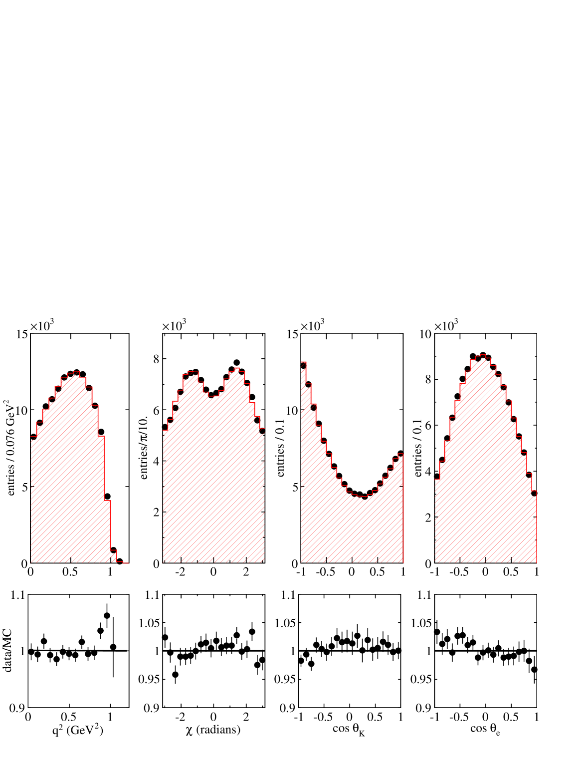
The total $\chi^{2}$ value is 2901 and the number of degrees of freedom is 2786. This corresponds to a probability of $6.4\%$ . Systematic uncertainties, evaluated as in Section VII.1, are given in Table 11. The statistical error matrix of fitted parameters, a table showing individual contribution of sources of systematic uncertainties, which were grouped in the entries of Tab. 11 labelled III, VII and XI, and the full error matrix of systematic uncertainties are given in A. Projected distributions versus the five variables obtained in data and from the fit result are displayed in Fig. 11. Measured and fitted distributions of the values of the $F_{cc}$ discriminant variable are compared in Fig. 12.

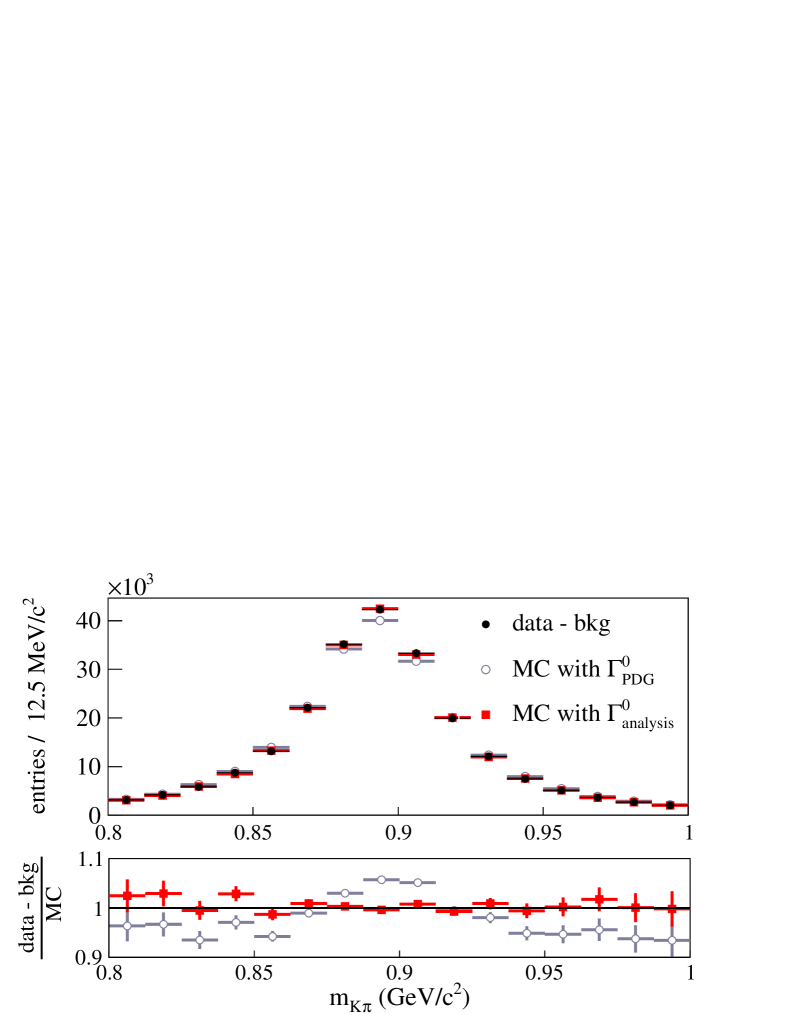
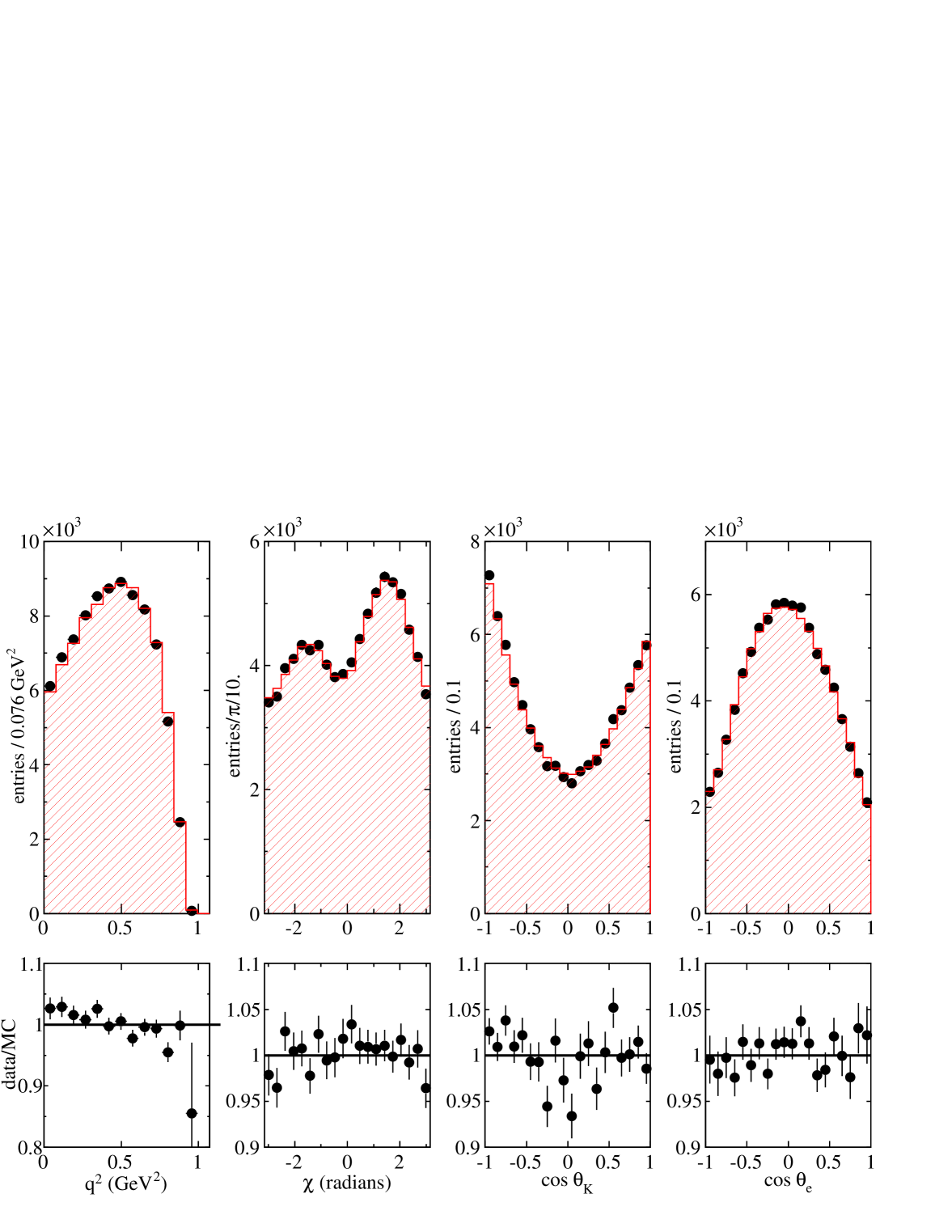
The comparison between measured and fitted, background subtracted, mass distributions is given in Fig. 13. Results of a fit in which the width of the $K^{*}(892)^{0}$ resonance is fixed to $50.3~{\mathrm{\,Me\kern-1.00006ptV\!/}c^{2}}$ (the value quoted in 2008 by the Particle Data Group) are also given.

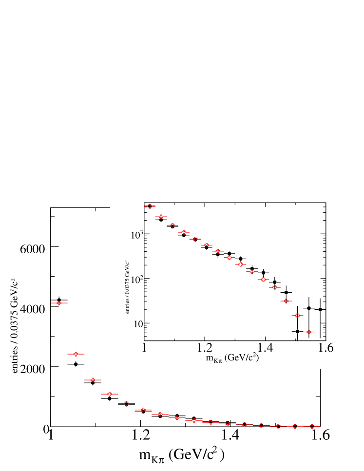
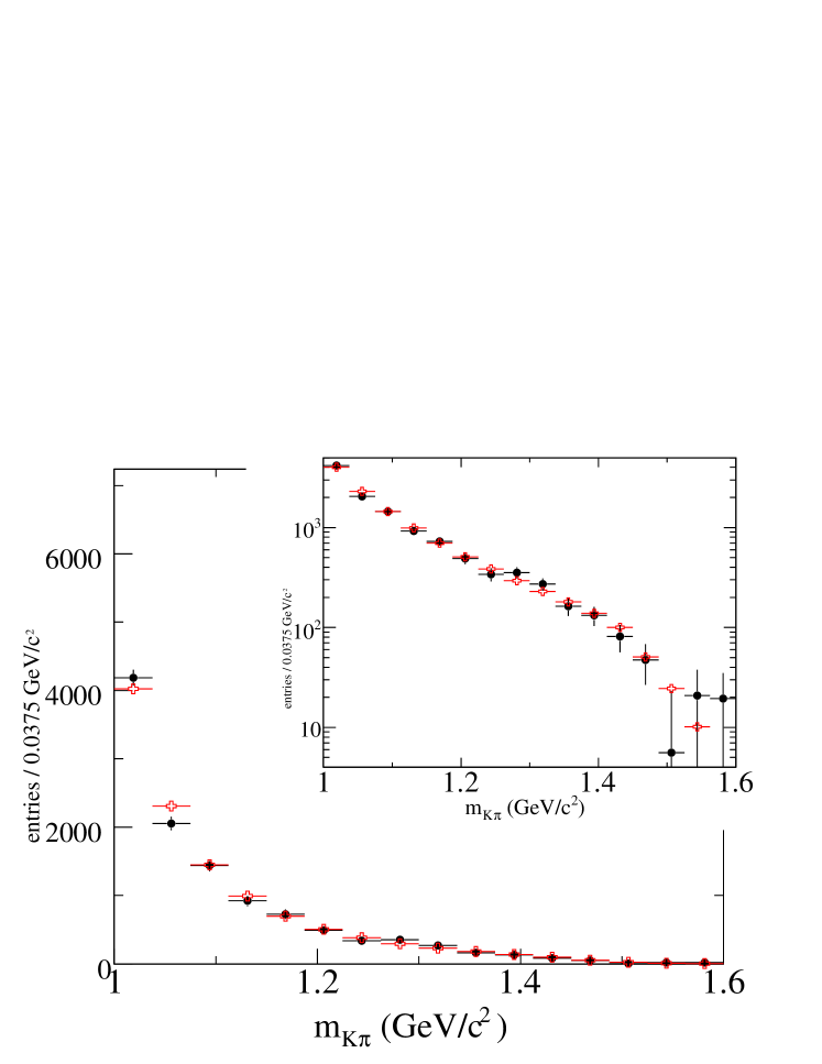
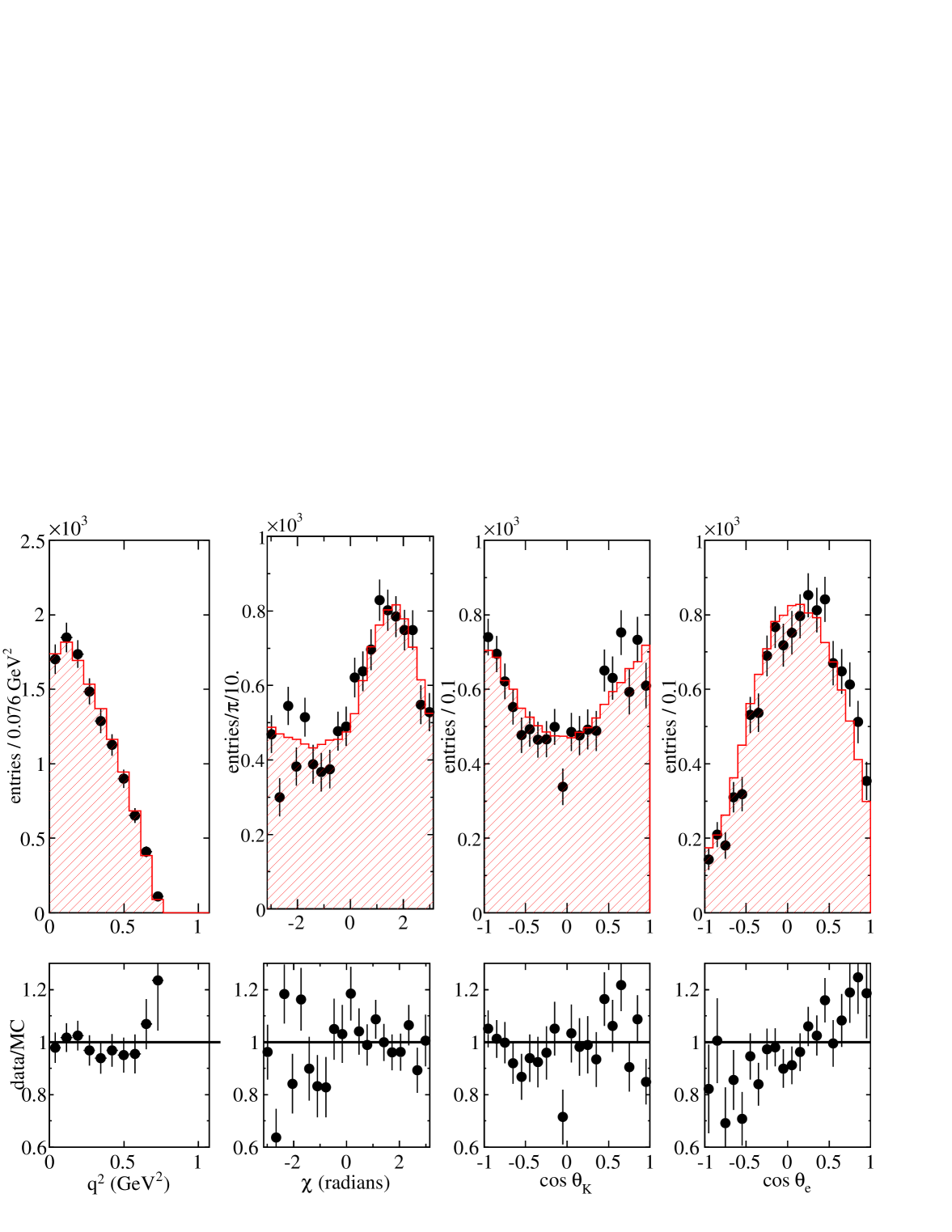
Background subtracted projected distributions versus $m_{K\pi}$ for values higher than 1 ${\mathrm{\,Ge\kern-1.00006ptV\!/}c^{2}}$ , obtained in data and using the fit results with and without including the $\overline{K}^{*}(1410)^{0}$ , are displayed in Fig. 14.

The measured fraction of the $\overline{K}^{*}(1410)^{0}$ is compatible with the value obtained in $\tau$ decays ref:taubelle . The relative phase between the $\overline{K}^{*}(892)^{0}$ and $\overline{K}^{*}(1410)^{0}$ is compatible with zero, as expected. Values of the hadronic form factor parameters for the decay $D^{+}\rightarrow\overline{K}^{*0}e^{+}\nu_{e}$ are almost identical with those obtained without including the $\overline{K}^{*}(1410)^{0}$ . The fitted value for $a_{S,BG}^{1/2}$ is compatible with the result from LASS reported in Table 3.

The total fraction of the $S$ -wave is compatible with the previous value. Fractions for each component are given in the third column of Table 9.

Considering several mass intervals, background subtracted projected distributions versus the four other variables, obtained in data and from the fit results, are displayed in Fig. 15 to 18.

Table 12: Systematic uncertainties on parameters fitted using a model for the signal which contains

S

-wave,

\overline{K}^{*}(892)^{0}

and

\overline{K}^{*}(1410)^{0}

components in which the

\overline{K}^{*}(892)^{0}

parameters are fixed, expressed as

(x[0]-x[i])/\sigma_{stat}

:: (I) uncertainty associated with the tuning of the signal control sample, (II) fraction of radiative signal events increased by

30\%

, (III) no PID correction on electron or kaon in MC signal events, (IV) no smearing applied on

\theta_{D},~\phi_{D}~{\rm and}~E_{miss}

for simulated signal events, (V)

B\overline{B}

background rate lowered by the statistical uncertainty of its determination, (VI) uncertainty associated with the tuning of fragmentation in charm background events, (VII) remaining uncertainty on semileptonic decay models for background events, (VIII) uncertainty associated with c-meson relative fractions, (IX) uncertainty remaining from the smoothing of the background distribution, (X) effects from limited statistics in simulation, (XI) variation of parameters that were kept constant in the fit, (XII) uncertainties on absolute mass scale.

variation	$\Delta r_{K^{*}(1410)^{0}}$	$\Delta\delta_{K^{*}(1410)^{0}}$	$\Delta r_{S}$	$\Delta r^{(1)}_{S}$	$\Delta\delta_{1}$	$\Delta\delta_{2}$	$\Delta\delta_{3}$	$\Delta\delta_{4}$	$\Delta\delta_{5}$	$\Delta\delta_{6}$	$\Delta\delta_{7}$	$\Delta\delta_{8}$	$\Delta\delta_{9}$
(I)	0.23	-0.08	-0.13	-0.16	0.02	-0.07	-0.09	0.08	0.05	-0.06	0.01	0.01	-0.09
(II)	-0.34	0.02	0	-0.03	0.04	0.01	-0.01	0.01	0.21	-0.14	-0.03	0.04	0.17
(III)	-0.01	-0.05	-0.11	-0.11	0.05	-0.03	-0.11	0.29	0.55	0.05	0.10	0.04	0.03
(IV)	-0.92	0.26	-0.12	-0.14	-0.08	0.12	0.02	-0.11	0	-0.21	-0.22	-0.03	0.50
$B\overline{B}$ bkg.
(V)	-1.05	0.17	-0.03	-0.08	0.17	0.21	0.27	0.14	-0.12	-0.36	-0.36	-0.19	0.59
$c\overline{c}$ bkg.
(VI)	-0.17	-0.01	0.16	0.12	-0.02	0.01	-0.01	0.01	0.01	-0.03	-0.05	-0.05	-0.08
(VII)	0.15	0.09	0.11	0.13	0.20	0.11	0.08	0.03	0.09	0.11	0.13	0.10	0.06
(VIII)	-2.85	-0.36	-0.22	-0.19	-0.12	-0.37	-0.1	0.59	0.82	0.27	0.15	0.14	1.29
Fitting procedure
(IX)	0.60	0.60	0.60	0.60	1.06	0.64	0.47	0.42	0.40	0.49	0.54	0.63	0.82
(X)	0.70	0.70	0.60	0.61	0.53	0.54	0.53	0.53	0.78	0.54	0.53	0.54	0.98
(XI)	1.07	0.27	0.23	0.26	0.16	0.07	0.09	0.16	0.28	0.16	0.14	0.14	0.53
(XII)	-0.49	0.01	-0.01	-0.04	-0.03	0.12	0	0.33	0.50	0.10	0.12	0.14	0.27
$\sigma_{syst}$	3.70	1.09	0.94	0.96	1.24	0.99	0.83	1.04	1.47	0.99	0.98	0.91	2.07

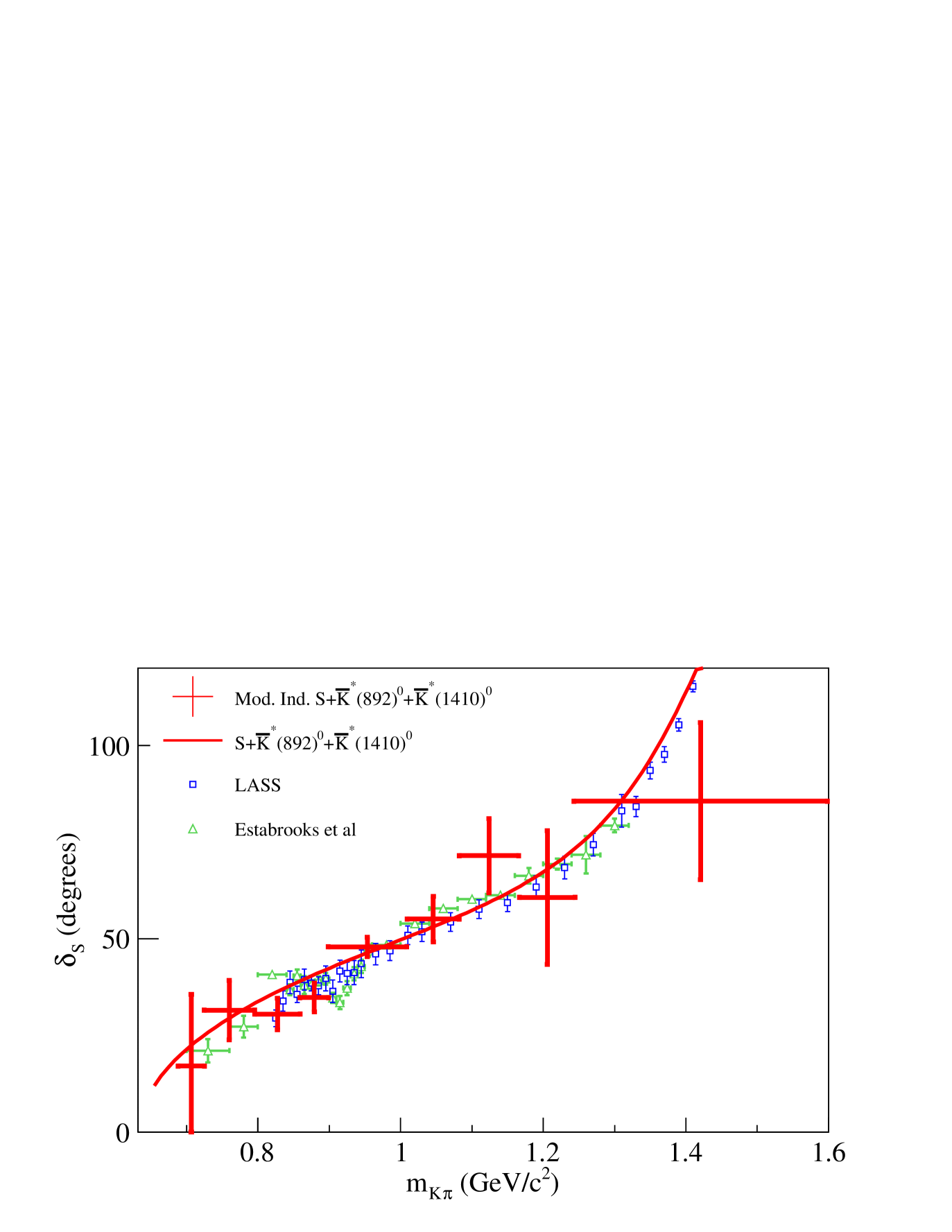
VIII.2 Fit of the $\overline{K}^{*}(1410)^{0}$ contribution and of the $S$ -wave amplitude and phase

Fixing the parameters which determine the $K^{*}(892)^{0}$ contribution to the values obtained in the previous fit, we measure the $S$ -wave parameters entering in Eq. (28) in which the $S$ -wave phase is assumed to be a constant within each of the considered $K\pi$ mass intervals.Values of $m_{K\pi}$ which correspond to the center and to half the width of each mass interval are given in Table 13. The two parameters which define the $\overline{K}^{*}(1410)^{0}$ are also fitted. Numbers of signal and background events are fixed to their previously determined values. Values of fitted parameters are given in Table 14.

Table 13: Positions of the center and values of half the mass intervals used in the phase measurement.

mass bin	$m_{K\pi}~({\mathrm{\,Ge\kern-1.00006ptV\!/}c^{2}})$	$\Delta m_{K\pi}~({\mathrm{\,Ge\kern-1.00006ptV\!/}c^{2}})$
$1$	0.707	0.019
$2$	0.761	0.035
$3$	0.828	0.032
$4$	0.880	0.020
$5$	0.955	0.055
$6$	1.047	0.037
$7$	1.125	0.041
$8$	1.205	0.039
$9$	1.422	0.178

Table 14: Fit results for a signal made of

S

-wave,

\overline{K}^{*}(892)^{0}

and

\overline{K}^{*}(1410)^{0}

components. The

S

-wave phase is measured for several values of the

K\pi

mass and its amplitude is parameterized according to Eq. (28). The two last columns give the values of the

P

-wave phase, which includes

\overline{K}^{*}(892)^{0}

and

\overline{K}^{*}(1410)^{0}

components, and the values of the difference between the

S

- and

P

-wave phases. Quoted uncertainties are statistical only, systematic uncertainties are given in Table 12. The same uncertainties apply to

\delta_{S}

and

\delta_{S}-\delta_{P}

variable	result
$r_{K^{*}(1410)^{0}}$	$0.079\pm 0.004$
$\delta_{K^{*}(1410)^{0}}(^{\circ})$	$-8.9\pm 21.5$
$r_{S}$	$0.463\pm 0.068$
$r^{(1)}_{S}$	$0.21\pm 0.18$
	$\delta_{S}(^{\circ})$	$\delta_{P}(^{\circ})$	$\delta_{S}-\delta_{P}(^{\circ})$
$\delta_{1}$	$16.8\pm 11.7$	2.0	14.8
$\delta_{2}$	$31.3\pm 5.5$	4.4	26.9
$\delta_{3}$	$30.4\pm 3.1$	13.6	16.9
$\delta_{4}$	$34.7\pm 2.6$	54.0	-19.3
$\delta_{5}$	$47.7\pm 1.4$	152.2	-104.4
$\delta_{6}$	$55.0\pm 4.2$	161.4	-106.4
$\delta_{7}$	$71.2\pm 6.9$	159.1	-87.9
$\delta_{8}$	$60.6\pm 12.8$	148.1	-87.5
$\delta_{9}$	$85.3\pm 8.8$	130.9	-45.6

The variation of the $S$ -wave phase is given in Fig. 19 and compared with LASS results and with the result found in Section VIII where the $S$ -wave phase variation was parameterized versus the $K\pi$ mass.

Systematic uncertainties are given in Table 12.

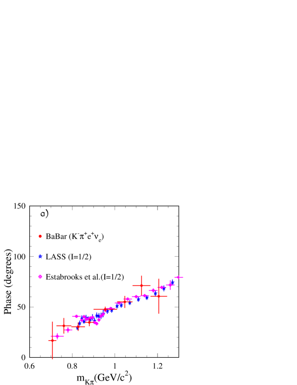
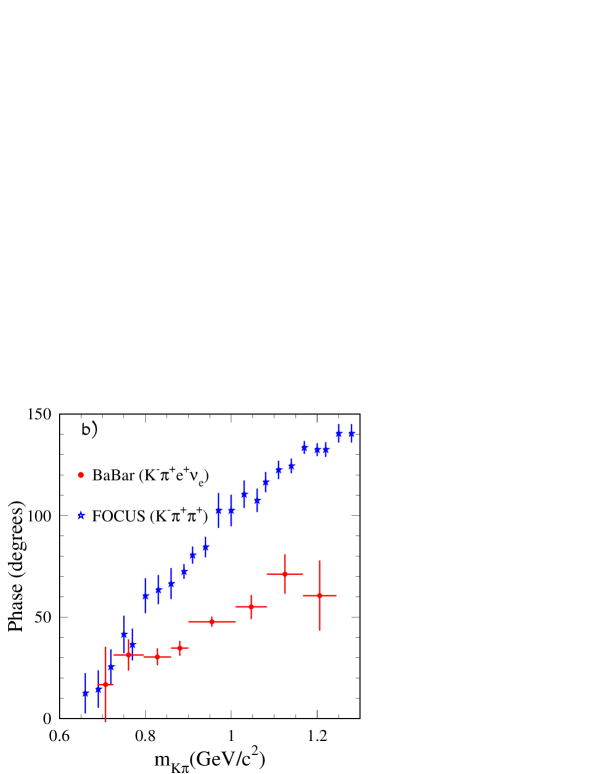
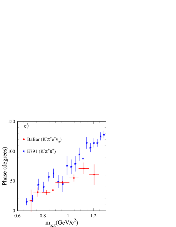
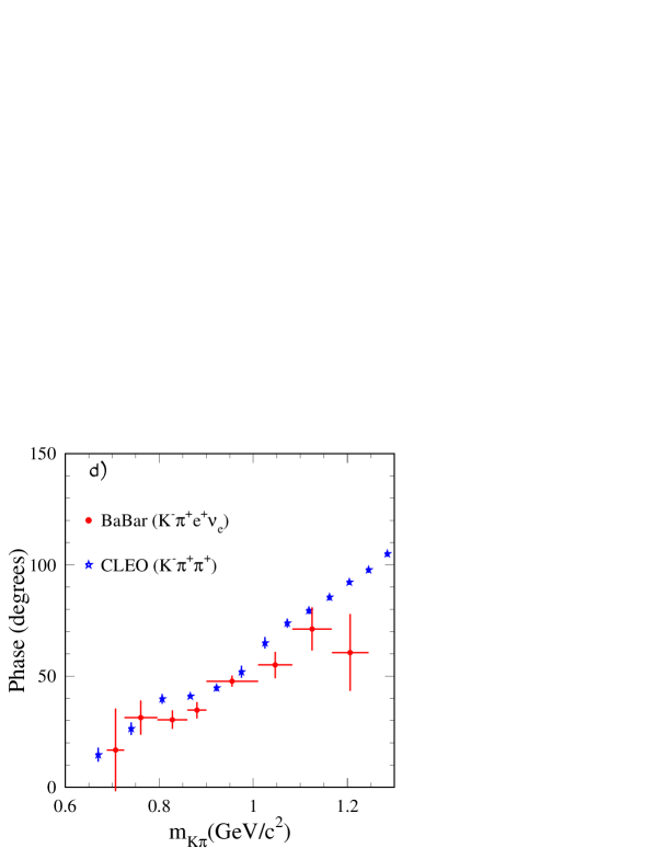
In Fig. 20 measured values of the $S$ -wave phase obtained by various experiments in the elastic region are compared. Fig. 20-a is a zoom of Fig. 19. Fig. 20-b to -d compare present measurements with those obtained in Dalitz plot analyses of the decay $D^{+}\rightarrow K^{-}\pi^{+}\pi^{+}$ . For the latter, the $S$ -wave phase is obtained by reference to the phase of the amplitude of one of the contributing channels in this decay. To draw the different figures it is assumed that the phase of the $S$ -wave is equal at $m_{K\pi}=0.67~{\mathrm{\,Ge\kern-1.00006ptV\!/}c^{2}}$ to the value given by the fitted parameterization on LASS data. It is difficult to draw clear conclusions from these comparisons as Dalitz plot analyses do not provide usually the phase of the $I=1/2$ amplitude alone but the phase for the total $S$ -wave amplitude.

VIII.3 $\delta_{S}-\delta_{P}$ measurement

As explained in previous sections, measurements are sensitive to the phase difference between $S$ - and $P$ -waves. This quantity is given in Fig. 21 for different values of the $K\pi$ mass using results from the fit explained in Section VIII.2. Similar values are obtained if the $\overline{K}^{*}(1410)^{0}$ is not included in the $P$ -wave.

VIII.4 Search for a $D$ -wave component

A $D$ -wave component, assumed to correspond to the $\overline{K}^{*}_{2}(1430)^{0}$ , is added in the signal model using expressions given in Eq. (IV) and (IV.3-32). As the phase of the $\overline{K}^{*}(1410)^{0}$ , relative to the $\overline{K}^{*}(892)^{0}$ , is compatible with zero this value is imposed in the fit. For the $D$ -wave, its phase $(\delta_{D})$ is allowed to be zero or $\pi$ . Fit results are given in the last column of Table 8. The total $\chi^{2}$ value is 2888 and the number of degrees of freedom is 2786. This corresponds to a probability of $8.8\%$ . The value zero is favored for $\delta_{D}$ . The fraction of the decay rate which corresponds to the $D$ wave is given in Table 9 and is similar to the $\overline{K}^{*}(1410)^{0}$ fraction.

IX Decay rate measurement

The $D^{+}\rightarrow K^{-}\pi^{+}e^{+}\nu_{e}(\gamma)$ branching fraction is measured relative to the reference decay channel, $D^{+}\rightarrow K^{-}\pi^{+}\pi^{+}(\gamma)$ . Specifically, in Eq. (IX) we compare the ratio of rates for the decays $D^{+}\rightarrow K^{-}\pi^{+}e^{+}\nu_{e}(\gamma)$ and $D^{+}\rightarrow K^{-}\pi^{+}\pi^{+}(\gamma)$ in data and simulated events: this way, many systematic uncertainties cancel:

$\displaystyle R_{D}$	$\displaystyle=$	$\displaystyle\frac{{\cal B}(D^{+}\rightarrow K^{-}\pi^{+}e^{+}\nu_{e})_{data}}{{\cal B}(D^{+}\rightarrow K^{-}\pi^{+}\pi^{+})_{data}}$
	$\displaystyle=$	$\displaystyle\frac{N(D^{+}\rightarrow K^{-}\pi^{+}e^{+}\nu_{e})_{data}}{\epsilon(K^{-}\pi^{+}e^{+}\nu_{e})_{data}}$
	$\displaystyle\times$	$\displaystyle\frac{\epsilon(K^{-}\pi^{+}\pi)_{data}}{N(D^{+}\rightarrow K^{-}\pi^{+}\pi^{+})_{data}}\times\frac{{\cal L}(K\pi\pi)_{data}}{{\cal L}(K\pi e\nu)_{data}}.$

Introducing the reconstruction efficiency measured for the two channels with simulated events, this expression can be written:

$\displaystyle R_{D}$	$\displaystyle=$	$\displaystyle\frac{N(D^{+}\rightarrow K^{-}\pi^{+}e^{+}\nu_{e})_{data}}{N(D^{+}\rightarrow K^{-}\pi^{+}\pi^{+})_{data}}\times\frac{{\cal L}(K\pi\pi)_{data}}{{\cal L}(K\pi e\nu_{e})_{data}}$	(41)
	$\displaystyle\times$	$\displaystyle\frac{\epsilon(K^{-}\pi^{+}e^{+}\nu_{e})_{MC}}{\epsilon(K^{-}\pi^{+}e^{+}\nu_{e})_{data}}\times\frac{\epsilon(K^{-}\pi^{+}\pi^{+})_{data}}{\epsilon(K^{-}\pi^{+}\pi^{+})_{MC}}$
	$\displaystyle\times$	$\displaystyle\frac{\epsilon(K^{-}\pi^{+}\pi^{+})_{MC}}{\epsilon(K^{-}\pi^{+}e^{+}\nu_{e})_{MC}}$

The first line in this expression is the product between the ratio of measured number of signal events in data for the semileptonic and hadronic channels, and the ratio of the corresponding integrated luminosities analyzed for the two channels:

\displaystyle\frac{{\cal L}(K\pi\pi)_{data}}{{\cal L}(K\pi e\nu_{e})_{data}}=\frac{98.7~\mbox{fb${}^{-1}$}}{100.5~\mbox{fb${}^{-1}$}}

(42)

The second line of Eq. (41) corresponds to the ratio between efficiencies in data and in simulation, for the two channels. The last line is the ratio between efficiencies for the two channels measured using simulated events. Considering that a special event sample is generated for the semileptonic decay channel, in which each event contains a decay $D^{+}\rightarrow\overline{K}^{*0}e^{+}\nu_{e},~\overline{K}^{*0}\rightarrow K^{-}\pi^{+}$ , whereas the $D^{+}\rightarrow K^{-}\pi^{+}\pi^{+}$ is reconstructed using the $e^{+}e^{-}\rightarrow c\overline{c}$ generic simulation, the last term in Eq. (41) is written:

	$\displaystyle\frac{\epsilon(K^{-}\pi^{+}\pi^{+})_{MC}}{\epsilon(\overline{K}^{0}e^{+}\nu_{e})_{MC}}=\frac{N(D^{+}\rightarrow K^{-}\pi^{+}\pi^{+})_{MC}}{N(D^{+}\rightarrow\overline{K}^{0}e^{+}\nu_{e})_{MC}}$		(43)
	$\displaystyle\times\frac{N(D^{+}\rightarrow\overline{K}^{*0}e^{+}\nu_{e})_{MC}^{gen}}{2N(c\bar{c})_{K\pi\pi}{\cal P}(c\rightarrow D^{+}){\cal B}(D^{+}\rightarrow K^{-}\pi^{+}\pi^{+})_{MC}}$

where:

•

$N(D^{+}\rightarrow\overline{K}^{*0}e^{+}\nu_{e})_{MC}^{gen}=1.17\times 10^{7}$ is the number of generated signal events;
•

$N(c\bar{c})_{K\pi\pi}=1.517\times 10^{8}$ is the number of $e^{+}e^{-}\rightarrow c\overline{c}$ events analyzed to reconstruct the $D^{+}\rightarrow K^{-}\pi^{+}\pi^{+}$ channel;
•

${\cal P}(c\rightarrow D^{+})=26.0\%$ is the probability that a $c$ -quark hadronizes into a $D^{+}$ in simulated events. The $D^{+}$ is prompt or is cascading from a higher mass charm resonance;
•

${\cal B}(D^{+}\rightarrow K^{-}\pi^{+}\pi^{+})_{MC}=0.0923$ is the branching fraction used in the simulation.

IX.1 Selection of candidate signal events

To minimize systematic uncertainties, common selection criteria are used, as much as possible, to reconstruct the two decay channels.

IX.1.1 The $D^{+}\rightarrow K^{-}\pi^{+}\pi^{+}$ decay channel

As compared to the semileptonic decay channel, the selection criteria described in Section VI.1 are used, apart for those involving the lepton. The number of signal candidates is measured from the $K^{-}\pi^{+}\pi^{+}$ mass distribution, after subtraction of events situated in sidebands. The signal region corresponds to the mass interval $[1.849,~1.889]~{\mathrm{\,Ge\kern-1.00006ptV\!/}c^{2}}$ whereas sidebands are selected within $[1.798,~1.838]$ and $[1.900,~1.940]~{\mathrm{\,Ge\kern-1.00006ptV\!/}c^{2}}$ . Results are given in Table 15 and an example of the $K^{-}\pi^{+}\pi^{+}$ mass distribution measured on data is displayed in Fig. 22.

The following differences between data and simulation are considered:

•

the signal mass interval.

Table 15: Measured numbers of signal events in data and simulation satisfying $F_{cc}>0.5$ .

Channel Data Simulation

$K^{-}\pi^{+}e^{+}\nu_{e}$ $70549\pm 363$ $330969$

$K^{-}\pi^{+}\pi^{+}$ $52595\pm 251$ $68468\pm 283$

Procedures have been defined in Section VI.3.5 such that the average mass and width of the $D^{+}\rightarrow K^{-}\pi^{+}\pi^{+}$ reconstructed signal in data and simulated events are similar.
•

the Dalitz plot model. Simulated events are generated using a model which differs from present measurements of the event distribution over the Dalitz plane. Measurements from CLEO-c ref:kpipi_cleoc are used to reweight simulated events and we measure that the number of reconstructed signal events changes by a factor $1.0017\pm 0.0038$ . This small variation is due to the approximately uniform acceptance of the analysis for this channel.
•

the pion track. As compared with the $K^{-}\pi^{+}e^{+}\nu_{e}$ final state, there is a $\pi^{+}$ in place of the $e^{+}$ in the reference channel. As there is no requirement on the PID for this pion we have considered that possible differences between data and simulation on tracking efficiency cancel when considering the simultaneous reconstruction of the pion and the electron. What remains is the difference between data and simulation for electron identification which is included in the evaluation of systematic uncertainties.

IX.1.2 The $D^{+}\rightarrow K^{-}\pi^{+}e^{+}\nu_{e}$ decay channel

The same data sample as used to measure the $D^{+}\rightarrow K^{-}\pi^{+}\pi^{+}$ is analyzed. Signal events are fitted as in Section VII. The stability of the measurement is verified versus the value of the cut on $F_{cc}$ which is varied between 0.4 and 0.7. Over this range the number of signal and background events change by factors 0.62 and 0.36 respectively. The variation of the ratio between the number of selected events,

R_{N}=\frac{N(D^{+}\rightarrow K^{-}\pi^{+}\pi^{+})_{MC}}{N(D^{+}\rightarrow\overline{K}^{*0}e^{+}\nu_{e})_{MC}}\frac{N(D^{+}\rightarrow K^{-}\pi^{+}e^{+}\nu_{e})_{data}}{N(D^{+}\rightarrow K^{-}\pi^{+}\pi^{+})_{data}}

(44)

in data and simulation is given in Table 16.

Table 16: Variation of the ratio between the numbers of selected events in data and simulation for different values of the cut on

F_{cc}

	$F_{cc}>0.4$	$F_{cc}>0.5$	$F_{cc}>0.7$
$N(D^{+}\rightarrow K^{-}\pi^{+}\pi^{+})_{MC}$	$72206\pm 292$	$60468\pm 283$	$59259\pm 259$
$N(D^{+}\rightarrow K^{-}\pi^{+}\pi^{+})_{data}$	$55361\pm 260$	$52595\pm 251$	$45627\pm 230$
$N(D^{+}\rightarrow\overline{K}^{*0}e^{+}\nu_{e})_{MC}$	$381707$	$330969$	$237104$
$N(D^{+}\rightarrow K^{-}\pi^{+}e^{+}\nu_{e})_{data}$	$81322\pm 383$	$70549\pm 363$	$50989\pm 303$
$R_{N}$	$0.2779\pm 0.022$	$0.2775\pm 0.0023$	$0.2793\pm 0.0026$

Relative to the value for the nominal cut ( $F_{cc}>0.5$ ), the value of $R_{N}$ for $F_{cc}>0.4$ is higher by $0.00038\pm 0.00063$ and for $F_{cc}>0.7$ it is higher by $0.0018\pm 0.0011$ . Quoted uncertainties take into account events that are common when comparing the samples. These variations are compatible with statistical fluctuations and no additional systematic uncertainty is included.

To select semileptonic decay candidates a cut is applied on the probability of the $D^{+}$ mass-constrained fit at $0.01$ . In a previous analysis of the decay $D^{0}\rightarrow K^{-}e^{+}\nu_{e}$ ref:kenu we measured a value of $1.0062\pm 0.0006$ for the ratio between the efficiency of this cut in simulation and data. We use the same value in the present analysis because this probability depends on the capability to reconstruct the $D$ direction and momentum and to estimate corresponding uncertainties on these quantities which are obtained, not from the studied decay channel, but from the rest of the event.

IX.2 Decay rate measurement

Measurement of the $D^{+}\rightarrow K^{-}\pi^{+}e^{+}\nu_{e}$ branching fraction and of the contributing $S-$ wave, $\overline{K}^{*}(892)^{0}$ , $\overline{K}^{*}(1410)^{0}$ and $\overline{K}^{*}_{2}(1430)^{0}$ components is important to verify if the sum of exclusive channels in $D$ -meson semileptonic decays agrees with the inclusive value. From the measurement of ${\cal B}(D^{+}\rightarrow\overline{K}^{*}(892)^{0}e^{+}\nu_{e})$ the value of $|A_{1}(0)|$ is obtained and provides, with $r_{2}$ and $r_{V}$ , the absolute normalization for the corresponding hadronic form factors. These values can be compared with Lattice QCD determinations.

Combining all measured quantities in Eq. (41), the relative decay rate is:

R_{D}=0.4380\pm 0.0036\pm 0.0042

(45)

where uncertainties are statistical and systematic respectively. Using the CLEO-c value for the branching fraction ${\cal B}(D^{+}\rightarrow K^{-}\pi^{+}\pi^{+})=(9.14\pm 0.20)\%$ ref:cleockpipi , gives:

{\cal B}(D^{+}\rightarrow K^{-}\pi^{+}e^{+}\nu_{e})=(4.00\pm 0.03\pm 0.04\pm 0.09)\times 10^{-2}

(46)

where the last quoted uncertainty comes from the accuracy of ${\cal B}(D^{+}\rightarrow K^{-}\pi^{+}\pi^{+})$ . To evaluate the contribution from the $\overline{K}^{*0}$ , results obtained with the $S+\overline{K}^{*}(892)^{0}+\overline{K}^{*}(1410)^{0}$ signal model are used. The branching fraction for $D^{+}\rightarrow\overline{K}^{*0}e^{+}\nu_{e}$ is obtained after subtracting the $S$ - and $\overline{K}^{*}(1410)^{0}$ -wave contributions:

		$\displaystyle{\cal B}(D^{+}\rightarrow\overline{K}^{0}e^{+}\nu_{e})\times{\cal B}(\overline{K}^{0}\rightarrow K^{-}\pi^{+})=$			(47)
		$\displaystyle(3.77\pm 0.04\pm 0.05\pm 0.09)\times 10^{-2}.$

The last uncertainty corresponds to external inputs.

The corresponding value of $A_{1}(0)$ is obtained by integrating Eq. (16), restricted to the $\overline{K}^{*0}$ contribution, over the three angles:

	$\displaystyle\frac{{\rm d}\Gamma}{{\rm d}q^{2}{\rm d}m^{2}}$	$\displaystyle=$	$\displaystyle\frac{1}{3}\frac{G_{F}^{2}\left\|\|V_{cs}\|\right\|^{2}}{\left(4\pi\right)^{5}m_{D}^{2}}\beta\,p_{K\pi}$		(48)
		$\displaystyle\times$	$\displaystyle\left[\frac{2}{3}\left\{\|{\cal F}_{11}\|^{2}+\|{\cal F}_{21}\|^{2}+\|{\cal F}_{31}\|^{2}\right\}\right]$		(48)

Assuming that the $K^{*}(892)^{0}$ meson is infinitely narrow, integrating over the remaining variables gives:

	$\displaystyle\Gamma$	$\displaystyle=$	$\displaystyle\frac{\hbar{\cal B}(D^{+}\rightarrow\overline{K}^{0}e^{+}\nu_{e}){\cal B}(\overline{K}^{0}\rightarrow K^{-}\pi^{+})}{\tau_{D^{+}}}$
		$\displaystyle=$	$\displaystyle\frac{G_{F}^{2}\left\|\|V_{cs}\|\right\|^{2}}{96\pi^{3}}\frac{2}{3}\|A_{1}(0)\|^{2}\cal I,$

with

	$\displaystyle{\cal I}$	$\displaystyle=$	$\displaystyle\int^{q^{2}max}_{0}\frac{p_{K\pi}\,q^{2}}{\|A_{1}(0)\|^{2}m_{D}^{2}}$		(50)
		$\displaystyle\times$	$\displaystyle\left[\|H_{0}\|^{2}+\|H_{+}\|^{2}+\|H_{-}\|^{2}\right]{\rm d}q^{2}$		(50)

and:

A_{1}(0)=0.6200\pm 0.0056\pm 0.0065\pm 0.0071.

(51)

For this last evaluation, the values $\tau_{D^{+}}=(10.40\pm 0.07)\times 10^{-13}s$ for the $D^{+}$ lifetime ref:pdg10 and $|V_{cs}|=0.9729\pm 0.0003$ are used. Corresponding uncertainties are included in the last quoted error in Eq. (51).

If instead of considering a $K^{*}(892)^{0}$ with zero width, the fitted mass distribution of the resonance is used in the integral of the differential decay rate versus $q^{2}$ and $m^{2}$ , the form factor normalization becomes:

A_{1}(0)|_{q^{2},m^{2}}=0.9174\pm 0.0084\pm 0.0097\pm 0.0105.

(52)

This value depends also on the normalization adopted for the mass distribution which is given in Eq. (26).

X Summary

We have studied the decay $D^{+}\rightarrow K^{-}\pi^{+}e^{+}\nu_{e}$ with a sample of approximately $244\times 10^{3}$ signal events, which greatly exceeds any previous measurement. The hadronic system in this decay is dominated by the $\overline{K}^{*0}$ meson. In addition to the $\overline{K}^{*0}$ meson we measure a contribution of the $K^{-}\pi^{+}$ $S$ -wave component of $(5.79\pm 0.16\pm 0.15)\%$ . We find a small contribution from the $\overline{K}^{*}(1410)^{0}$ equal to $(0.33\pm 0.13\pm 0.19)\%$ . This value agrees with the naive expectation based on corresponding measurements in $\tau$ decays. The relative phase between the $\overline{K}^{*}(892)^{0}$ and $\overline{K}^{*}(1410)^{0}$ components is compatible with zero whereas there is a negative sign between the $S$ - and $P$ -wave amplitudes. A fit to data of similar probability is obtained including a $D$ -wave component with a fraction equal to $(0.19\pm 0.09\pm 0.09)\%$ . In this case the $\overline{K}^{*}(1410)^{0}$ fraction becomes $(0.16\pm 0.08\pm 0.14)\%$ . As these two components do not exceed a significance of three standard deviations, upper limits at the 90 $\%$ C.L. are quoted in Table 17.

Using a model for signal which includes $S$ -wave, $\overline{K}^{*}(892)^{0}$ - and $\overline{K}^{*}(1410)^{0}$ contributions, hadronic form factor parameters of the $\overline{K}^{*0}$ component are obtained from a fit to the five-dimensional decay distribution, assuming single pole dominance: $r_{V}=V(0)/A_{1}(0)=1.463\pm 0.017\pm 0.032$ , $r_{2}=A_{2}(0)/A_{1}(0)=0.801\pm 0.020\pm 0.020$ and the pole mass of the axial vector form factors $m_{A}=\left(2.63\pm 0.10\pm 0.13\right)~{\mathrm{\,Ge\kern-1.00006ptV\!/}c^{2}}$ . For comparison with previous measurements we also perform a fit to data with fixed pole mass $m_{A}=2.5~{\mathrm{\,Ge\kern-1.00006ptV\!/}c^{2}}$ and $m_{V}=2.1~{\mathrm{\,Ge\kern-1.00006ptV\!/}c^{2}}$ and including only the $S$ and $\overline{K}^{*}(892)^{0}$ signal components; it gives $r_{V}=1.493\pm 0.014\pm 0.021$ and $r_{2}=0.775\pm 0.011\pm 0.011$ .

We have measured the phase of the $S$ -wave component for several values of the $K^{-}\pi^{+}$ mass. Contrary to similar analyses using charm meson decays, as in $D^{+}\rightarrow K^{-}\pi^{+}\pi^{+}$ , we find agreement with corresponding $S$ -wave phase measurements done in $K^{-}p$ interactions producing $K^{-}\pi^{+}$ at small transfer. This is a confirmation of these results and illustrates the importance of final state interactions in $D$ -meson hadronic decays. As compared with elastic $K^{-}\pi^{+}$ scattering there is an additional negative sign between the $S$ - and $P$ -wave, in the $D^{+}$ semileptonic decay channel. This observation does not contradict the Watson theorem. We have determined the parameters of the $K^{*}(892)^{0}$ meson and found, in particular, a width smaller than the value quoted in ref:pdg10 . Our result agrees with recent measurements from FOCUS ref:focus1 , CLEO ref:kpipi_cleoc and, $\tau$ decays (for the charged mode) ref:taubelle . Comparison between these measurements and present world average values is illustrated in Tab. 17. Our measurements of the $S$ -wave phase have large uncertainties in the threshold region and it remains to evaluate how they can improve the determination of chiral parameters using, for instance, the framework explained in ref. ref:seb1 .

Table 17: Comparison between these measurements and present world average results. Values for

{\cal B}(D^{+}\rightarrow\overline{K}^{*}(1410)^{0}/\overline{K}^{*}_{2}(1430)^{0}e^{+}\nu_{e})

are corrected for their respective branching fractions into

K^{-}\pi^{+}

Measured quantity	This analysis	World average ref:pdg10
$m_{K^{*}(892)^{0}}({\mathrm{\,Me\kern-1.00006ptV\!/}c^{2}})$	$895.4\pm{0.2}\pm 0.2$	$895.94\pm{0.22}$
$\Gamma^{0}_{K^{*}(892)^{0}}({\mathrm{\,Me\kern-1.00006ptV\!/}c^{2}})$	$46.5\pm{0.3}\pm 0.2$	$48.7\pm{0.8}$
$r_{BW}({\mathrm{\,Ge\kern-1.00006ptV\!/}c})^{-1}$	$2.1\pm{0.5}\pm 0.5$	$3.4\pm{0.7}$ ref:lass1
$r_{V}$	$1.463\pm{0.017}\pm 0.031$	$1.62\pm{0.08}$
$r_{2}$	$0.801\pm{0.020}\pm 0.020$	$0.83\pm{0.05}$
$m_{A}({\mathrm{\,Ge\kern-1.00006ptV\!/}c^{2}})$	$2.63\pm 0.10\pm 0.13$	no result
${\cal B}(D^{+}\rightarrow K^{-}\pi^{+}e^{+}\nu_{e})(\%)$	$4.00\pm 0.03\pm 0.04\pm 0.09$	$4.1\pm 0.6$
${\cal B}(D^{+}\rightarrow K^{-}\pi^{+}e^{+}\nu_{e})_{\overline{K}^{*}(892)^{0}}(\%)$	$3.77\pm 0.04\pm 0.05\pm 0.09$	$3.68\pm 0.21$
${\cal B}(D^{+}\rightarrow K^{-}\pi^{+}e^{+}\nu_{e})_{S-wave}(\%)$	$0.232\pm 0.007\pm 0.007\pm 0.005$	$0.21\pm 0.06$
${\cal B}(D^{+}\rightarrow\overline{K}^{*}(1410)^{0}e^{+}\nu_{e})(\%)$	$0.30\pm 0.12\pm 0.18\pm 0.06$ ( $<0.6$ at 90 $\%$ C.L.)
${\cal B}(D^{+}\rightarrow\overline{K}^{*}_{2}(1430)^{0}e^{+}\nu_{e})(\%)$	$0.023\pm 0.011\pm 0.011\pm 0.001$ ( $<0.05$ at 90 $\%$ C.L.)

XI Acknowledgments

The authors would like to thank S. Descotes-Genon and A. Le Yaouanc for fruitful discussions especially on the charm meson semileptonic decay rate formalism. We also thank V. Bernard, B. Moussallam and E. Passemar for discussions on chiral perturbation theory and different aspects of the $K\pi$ system.

We are grateful for the extraordinary contributions of our PEP-II colleagues in achieving the excellent luminosity and machine conditions that have made this work possible. The success of this project also relies critically on the expertise and dedication of the computing organizations that support BABAR. The collaborating institutions wish to thank SLAC for its support and the kind hospitality extended to them. This work is supported by the US Department of Energy and National Science Foundation, the Natural Sciences and Engineering Research Council (Canada), the Commissariat à l’Energie Atomique and Institut National de Physique Nucléaire et de Physique des Particules (France), the Bundesministerium für Bildung und Forschung and Deutsche Forschungsgemeinschaft (Germany), the Istituto Nazionale di Fisica Nucleare (Italy), the Foundation for Fundamental Research on Matter (The Netherlands), the Research Council of Norway, the Ministry of Education and Science of the Russian Federation, Ministerio de Ciencia e Innovación (Spain), and the Science and Technology Facilities Council (United Kingdom). Individuals have received support from the Marie-Curie IEF program (European Union), the A. P. Sloan Foundation (USA) and the Binational Science Foundation (USA-Israel).

Appendix A Error matrices for the nominal fit

The correlation matrix between statistical uncertainties is given in Tab. 18 for parameters fitted using the nominal model. Statistical uncertainties are quoted on the diagonal. The elements of the statistical error matrix are equal to $\rho_{ij}\,\sigma_{i}\,\sigma_{j}$ , where $\rho_{ij}$ is an off diagonal element or is equal to 1 on the diagonal.

Table 18: Correlation matrix for the

S+\overline{K}^{*}(892)^{0}+K^{*}(1410)^{0}

nominal fit. On the diagonal, statistical uncertainties (

\sigma_{i}^{stat.}

) of fitted quantities (

i

) are given.

$\Delta M_{K^{*}(892)^{0}}$	$\Delta\Gamma_{K^{*}(892)^{0}}$	$\Delta r_{BW}$	$\Delta m_{A}$	$\Delta r_{V}$	$\Delta r_{2}$	$\Delta r_{S}$	$\Delta r^{(1)}_{S}$	$\Delta a_{S,BG}^{1/2}$	$\Delta r_{K^{*}(1410)^{0}}$	$\Delta\delta_{K^{*}(1410)^{0}}$	$\Delta N_{S}$	$\Delta N_{B}$
0.211	0.656	-0.842	-0.158	0.142	-0.131	0.116	-0.043	-0.673	0.899	-0.774	-0.254	0.304
	0.315	-0.614	-0.002	0.020	0.007	0.007	0.024	-0.470	0.624	-0.632	0.027	-0.021
		0.476	0.163	-0.165	0.141	-0.347	0.270	0.657	-0.907	0.846	0.334	-0.394
			0.0972	-0.548	0.840	-0.045	-0.070	0.065	-0.080	0.087	0.099	-0.118
				0.0166	-0.518	0.048	0.034	-0.060	0.101	-0.126	-0.124	0.136
					0.0201	-0.016	-0.080	0.051	-0.058	0.080	0.116	-0.133
						0.0286	-0.968	-0.157	0.191	-0.048	-0.136	0.159
							0.0640	0.130	-0.133	-0.043	0.146	-0.173
								0.138	-0.767	0.396	0.148	-0.179
									0.0163	-0.721	-0.269	0.318
										13.0	0.288	-0.336
											713.0	-0.609
												613.2

In Tab. 11, systematic uncertainties quoted in lines labelled III, VII and XI are the result of several contributions, combined in quadrature. In Tab. 19 these components are detailed because each contribution can induce a positive or a negative variation of the fitted quantities.

Table 19: Systematic uncertainties on parameters fitted using a model for the signal which contains

S

-wave,

\overline{K}^{*}(892)^{0}

and

\overline{K}^{*}(1410)^{0}

components, expressed as

(x[0]-x[i])/\sigma_{stat}

: (IIIa) uncertainty associated with electron identification, (IIIb) uncertainty associated with kaon identification, (VIIa) : pole mass changed by -30

{\mathrm{\,Me\kern-1.00006ptV\!/}c^{2}}

for the decay channel

D^{0}\rightarrow K^{-}e^{+}\nu_{e}

, (VIIb) : pole mass changed by -100

{\mathrm{\,Me\kern-1.00006ptV\!/}c^{2}}

for semileptonic decays of

D^{0}

and

D^{+}

into a pseudoscalar meson, (VIIc) : pole mass changed by 100

{\mathrm{\,Me\kern-1.00006ptV\!/}c^{2}}

for

D_{s}

meson semileptonic decays, (VIId-j) refer to

D\rightarrow V~e^{+}\nu_{e}

decays; (VIId) :

r_{2}

changed from 0.80 to 0.85, (VIIe) :

r_{V}

changed from 1.50 to 1.55, (VIIf) :

m_{A}

changed from 2.5 to 2.2

{\mathrm{\,Ge\kern-1.00006ptV\!/}c^{2}}

, (VIIg) :

m_{V}

changed from 2.1 to 1.9

{\mathrm{\,Ge\kern-1.00006ptV\!/}c^{2}}

, (VIIh) :

r_{BW}

changed from 3.0 to 3.3

\mathrm{\,Ge\kern-1.00006ptV}^{-1}

, (VIIi) :

\Gamma_{K^{*}(892)^{0}}

varied by

-0.5~{\mathrm{\,Me\kern-1.00006ptV\!/}c^{2}}

, (XIa-d) :

K^{*}(1410)^{0}

mass and width,

K^{*}_{0}(1430)^{0}

mass and width in this order and using the variations given in Tab. 1 and, (XIe) :

m_{V}

changed by

100~{\mathrm{\,Me\kern-1.00006ptV\!/}c^{2}}

variation	$\Delta M_{K^{*}(892)^{0}}$	$\Delta\Gamma_{K^{*}(892)^{0}}$	$\Delta r_{BW}$	$\Delta m_{A}$	$\Delta r_{V}$	$\Delta r_{2}$	$\Delta r_{S}$	$\Delta r^{(1)}_{S}$	$\Delta a_{S,BG}^{1/2}$	$\Delta r_{K^{*}(1410)^{0}}$	$\Delta\delta_{K^{*}(1410)^{0}}$	$\Delta N_{S}$	$\Delta N_{B}$
$III$
a	0.02	0.03	-0.03	0.70	-0.73	0.50	0.12	-0.07	0.30	0.07	-0.20	0.07	-0.08
b	0.00	-0.10	0.05	-0.07	-0.05	-0.17	-0.07	0.01	-0.28	0.05	0.10	-0.07	0.08
$VII$
a	0.06	0.06	-0.05	-0.10	-0.05	0.01	0.17	-0.15	0.01	0.07	0.02	0.05	-0.06
b	0.01	0.01	-0.01	0.00	-0.01	0.01	0.01	-0.01	0.00	0.01	-0.01	0.00	-0.01
c	-0.01	0.00	0.01	-0.01	0.00	0.00	-0.01	0.01	0.00	-0.01	0.00	0.00	0.01
d	-0.03	0.00	0.06	0.00	0.02	0.05	0.01	-0.02	0.02	-0.02	0.04	0.06	-0.07
e	-0.03	-0.01	0.05	0.03	0.07	0.03	-0.02	0.01	0.01	-0.03	0.04	0.01	-0.01
f	0.00	0.03	0.07	-0.16	0.07	-0.03	0.01	-0.01	0.05	0.01	0.04	0.12	-0.15
g	-0.04	-0.01	0.06	0.03	0.08	0.04	-0.02	0.01	0.02	-0.04	0.05	0.02	-0.03
h	-0.06	-0.04	0.02	0.00	0.00	0.00	0.00	0.00	0.02	-0.04	0.06	0.00	0.00
i	-0.02	-0.02	0.01	-0.00	0.00	0.01	0.00	-0.01	0.00	-0.00	0.00	0.01	-0.01
$XI$
a	-0.08	-0.02	0.08	0.00	0.01	0.00	-0.35	0.34	-1.00	-0.34	-0.20	-0.04	0.05
b	0.20	0.09	-0.21	0.03	-0.03	0.03	0.44	-0.41	3.09	0.62	0.28	0.07	-0.08
c	-0.06	-0.02	0.08	0.01	-0.01	0.01	0.08	-0.10	0.05	-0.39	-0.08	0.02	-0.02
d	-0.16	-0.07	0.17	0.01	-0.01	0.01	0.05	-0.06	0.11	0.37	0.18	0.02	-0.03
e	0.00	0.00	-0.01	-0.06	-1.15	-0.07	0.04	-0.03	-0.01	0.00	0.00	0.01	-0.01

The error matrix for systematic uncertainties on fitted parameters is obtained using values of the variations given in Tab. 11 and 19. For each individual source of systematic uncertainty we create a matrix of elements equal to the product $\delta_{i}\,\delta_{j}$ of the variations observed on the values of the fitted parameters $i$ and $j$ . For systematic uncertainties IX and X, which have a statistical origin, we multiply these quantities by the corresponding elements of the statistical correlation matrix (Tab. 18). These matrices are summed to obtain the matrix given in Tab. 20.

Table 20: Correlation matrix for systematic uncertainties of the

S+\overline{K}^{*}(892)^{0}+K^{*}(1410)^{0}

nominal fit. On the diagonal, total systematic uncertainties (

\sigma_{i}^{syst.}

) on fitted quantities (

i

), are given.

$\Delta M_{K^{*}(892)^{0}}$	$\Delta\Gamma_{K^{*}(892)^{0}}$	$\Delta r_{BW}$	$\Delta m_{A}$	$\Delta r_{V}$	$\Delta r_{2}$	$\Delta r_{S}$	$\Delta r^{(1)}_{S}$	$\Delta a_{S,BG}^{1/2}$	$\Delta r_{K^{*}(1410)^{0}}$	$\Delta\delta_{K^{*}(1410)^{0}}$	$\Delta N_{S}$	$\Delta N_{B}$
0.226	0.569	-0.827	-0.004	0.153	-0.068	-0.080	0.115	0.038	0.731	-0.384	-0.422	0.439
	0.241	-0.579	0.081	0.065	0.049	-0.113	0.137	0.001	0.436	-0.400	-0.147	0.159
		0.540	-0.102	-0.182	-0.027	0.125	-0.153	-0.045	-0.728	0.470	0.620	-0.642
			0.124	-0.095	0.697	-0.279	0.260	0.071	0.029	0.044	-0.216	0.229
				0.0308	-0.367	-0.358	0.360	-0.080	0.063	0.179	-0.264	0.276
					0.0197	0.082	-0.102	0.110	0.022	-0.186	-0.067	0.067
						0.0406	-0.988	0.407	0.119	-0.078	0.461	-0.484
							0.0810	-0.395	-0.096	0.035	-0.448	0.471
								0.474	0.357	0.335	0.121	-0.126
									0.0222	-0.137	-0.346	0.355
										13.2	0.158	-0.155
											1055.2	-0.918
												1033.8

References

(1) S. Descotes-Genon and B. Moussallam, Eur. Phys. Jour. C 48, 553 (2006).
(2) M. Jamin and M. Münz, Z. Phys. C 66, 633 (1995).
(3) P. Colangelo, F. De Fazio, G. Nardulli and N. Paver, Phys. Lett. B 408, 340 (1997).
(4) P. Estabrooks et al., Nucl. Phys. B 133, 490 (1978).
(5) D. Aston et al., Nucl. Phys. B 296, 493 (1988).
(6) E.M. Aitala et al. (Fermilab E791 Collaboration), Phys. Rev. D 73, 032004 (2006).
(7) J.M. Link et al. (FOCUS Collaboration), Phys. Lett. B 653, 1 (2007).
(8) J.M. Link et al. (FOCUS Collaboration), Phys. Lett. B 681, 14 (2009).
(9) A. Bonvicini et al. (CLEO Collaboration), Phys. Rev. D 78, 052001 (2008).
(10) B. Aubert et al. (BABAR Collaboration), Phys. Rev. D 71, 032005 (2005).
(11) B. Aubert et al. (BABAR Collaboration), Nucl. Phys. Proc. Suppl. 189, 193 (2009).
(12) D. Epifanov et al. (Belle Collaboration), Phys. Lett. B 654, 65 (2007).
(13) P.L. Frabetti et al. (E687 Collaboration), Phys. Lett. B 307, 262 (1993).
(14) J.M. Link et al. (FOCUS Collaboration), Phys. Lett. B 535, 43 (2002).
(15) M.R. Shepherd et al. (CLEO Collaboration), Phys. Rev. D 74, 052001 (2006).
(16) K. Nakamura et al. (Particle Data Group), J. Phys. G37, 075021 (2010).
(17) V. Bernard, N. Kaiser and Ulf-G. Meissner, Nucl. Phys. B 357, 129 (1991); V. Bernard, N. Kaiser and Ulf-G. Meissner, Phys. Rev. D 43, 2757 (1991).
(18) J. Bijnens, P. Dhonte and P. Talavera, JHEP 0405:036, (2004).
(19) P. Büttiker, S. Descotes-Genon, B. Moussallam, Eur. Phys. Jour. C 33, 409 (2004).
(20) K.M. Watson, Phys. Rev. 95, 228 (1954); “Dynamics of the Standard Model”, J.F. Donoghue, E. Golowich and B.R. Holstein, Cambridge University Press (July 29, 1994).
(21) We thank A. Le Yaouanc for enlighting discussions about this point as, usually, it is considered that the Watson theorem implies a strict equality of the phases for the two processes.
(22) M. Jamin, A. Pich and J. Portoleś, Nucl. Phys. B 622, 279 (2002).
(23) W. Dunwoodie, private communication.
(24) M. Jamin, A. Pich and J. Portoleś, Phys. Lett. B 664, 78 (2008).
(25) B. Moussallam, Eur. Phys. Jour. C 53, 401 (2008).
(26) J.M. Link et al. (FOCUS Collaboration), Phys. Lett. B 621, 72 (2005).
(27) The convention used by FOCUS to define the Breit-Wigner amplitude differs by a (-) sign from the “usual” expression. By “usual” it is meant a phase which grows from zero to $\pi$ when the mass increases and which is equal to $\pi/2$ at the pole. In the present analysis we adopt this “usual” definition (Eq. (25)) which is also used in Ref. ref:pdg10 .
(28) E.M. Aitala et al. (E791 Collaboration), Phys. Rev. Lett. 89, 121801 (2002).
(29) C.L.Y. Lee, M. Lu and M.B. Wise, Phys. Rev. D 46, 5040 (1992).
(30) N. Cabibbo and A. Maksymowicz, Phys. Rev. 137, B438 (1965).
(31) A. Pais and S. B. Treiman, Phys. Rev. 168, 1858 (1968).
(32) J.D. Richman and P.R. Burchat, Rev. Mod. Phys. 67, 893 (1995).
(33) S. Fajfer and J. Kamenik, Phys. Rev. D 72, 034029 (2005);
D. Becirevic and A.B. Kaidalov, Phys. Lett. B 478, 417 (2000).
(34) S. Descotes-Genon, private communication.
(35) A.K. Leibovich, Z. Ligeti, I.W. Stewart and M.B. Wise, Phys. Rev. D 57, 308 (1998);
J. Charles, A. LeYaouanc, L. Oliver, O. Pene, J.C. Raynal, Phys. Rev. D 60, 014001 (1999);
A. Datta et al., Phys. Rev. D 77, 114025 (2008).
(36) B. Aubert et al. (BABAR Collaboration), Nucl. Instrum. Methods Phys. Res., Sect. A 479, 1 (2002).
(37) B. Aubert et al. (BABAR Collaboration), Phys. Rev. D 66, 032003 (2002).
(38) S. Agostinelli et al., Nucl. Instrum. Methods Phys. Res., Sect. A 506, 250 (2003).
(39) T. Sjöstrand , Comput. Phys. Commun. 82, 74 (1994).
(40) E. Barberio and Z. Was, Comput. Phys. Commun. 79, 291 (1994).
(41) B. Aubert et al. (BABAR Collaboration), Phys. Rev. D 76, 052005 (2007).
(42) B. Aubert et al. (BABAR Collaboration), Phys. Rev. D 78, 051101 (2008).
(43) G.C. Fox and S. Wolfram, Phys. Rev. Lett. 41, 1581 (1978).
(44) The hemisphere mass is the mass of the system corresponding to the sum of the 4-vectors of particles contained in that hemisphere.
(45) R. A. Fisher, Annals of Eugenics,7, p. 179-188 (1936).
(46) D. Scora and N. Isgur, Phys. Rev. D 52, 2783 (1995).
(47) J.D. Lange, Nucl. Instr. Meth. Phys. Res. Sect. A 462, 152 (2001).
(48) J.Y. Ge et al. (CLEO Collaboration), Phys. Rev. D 79, 052010 (2009).
(49) K. Cranmer, Kernel Estimation in high energy physics, Comput. Phys. Commun. 136, 198 (2001).
(50) T.C. Andre, Ann. Phys. 322, 2518 (2007).
(51) S. Dobbs et al. (CLEO Collaboration), Phys. Rev. D 77, 112005 (2008).
(52) S. Dobbs et al. (CLEO Collaboration), Phys. Rev. D 76, 112001 (2007).

Channel	Data	Simulation
$K^{-}\pi^{+}e^{+}\nu_{e}$	$70549\pm 363$	$330969$
$K^{-}\pi^{+}\pi^{+}$	$52595\pm 251$	$68468\pm 283$

Analysis of the D+→K−​π+​e+​νeD^{+}\rightarrow K^{-}\pi^{+}e^{+}\nu_{e} decay channel

Abstract

pacs:

I Introduction

II The K​πK\pi system in the elastic regime region

III Previous measurements

III.1 K​πK\pi production at small momentum transfer

III.2 τ−→K​π​ντ\tau^{-}\rightarrow K\pi\nu_{\tau} decays

III.3 Hadronic DD meson decays

III.4 Dℓ​4D_{\ell 4} decays

IV D+→K−​π+​e+​νeD^{+}\rightarrow K^{-}\pi^{+}e^{+}\nu_{e} decay rate formalism

IV.1 PP-wave form factors

IV.2 SS-wave form factor

IV.3 DD-wave form factors

V The BABAR detector and dataset

VI Analysis method

VI.1 Signal Selection

VI.2 Background rejection

VI.3 Simulation tuning

VI.3.1 Background from Υ​(4​S)\mathchar 28935\relax{(4S)} decays

VI.3.2 Simulation tuning of signal events

control of the c→D+c\rightarrow D^{+} production mechanism:

control of the D+D^{+} direction and missing energy measurements:

VI.3.3 Simulation tuning of charm background events from continuum

Corrections on charm quark hadronization:

Correction of D semileptonic decay form factors:

VI.3.4 Wrong sign event analysis

VI.3.5 Absolute mass scale.

VI.4 Fitting procedure

VI.4.1 Background smoothing

VII D+→K¯∗0​e+​νeD^{+}\rightarrow\overline{K}^{*0}e^{+}\nu_{e} hadronic form factor measurements

VII.1 Systematic uncertainties

VII.1.1 Signal production and decay

Corrections of distributions of Fisher input variables (I):

Simulation of radiative events (II):

Particle identification efficiencies (III):

Estimates of the values and uncertainties for the DD direction and missing energy (IV):

VII.1.2 B​B¯B\overline{B} background correction (V)

VII.1.3 Corrections to the c​c¯c\bar{c} background

Fragmentation associated systematic uncertainties (VI):

Form-factor correction systematics (VII):

Hadronization-associated systematic uncertainties (VIII):

VII.1.4 Fitting procedure

Background Smoothing (IX):

Limited statistics of simulated events (X):

VII.1.5 Parameters kept constant in the fit (XI).

VII.1.6 Absolute mass scale (XII).

VII.1.7 Comments on systematic uncertainties

VIII Including other components

VIII.1 Results with a K¯∗​(1410)0\overline{K}^{*}(1410)^{0} contribution included

VIII.2 Fit of the K¯∗​(1410)0\overline{K}^{*}(1410)^{0} contribution and of the SS-wave amplitude and phase

VIII.3 δS−δP\delta_{S}-\delta_{P} measurement

VIII.4 Search for a DD-wave component

IX Decay rate measurement

IX.1 Selection of candidate signal events

IX.1.1 The D+→K−​π+​π+D^{+}\rightarrow K^{-}\pi^{+}\pi^{+} decay channel

IX.1.2 The D+→K−​π+​e+​νeD^{+}\rightarrow K^{-}\pi^{+}e^{+}\nu_{e} decay channel

IX.2 Decay rate measurement

X Summary

XI Acknowledgments

Appendix A Error matrices for the nominal fit

References

Analysis of the $D^{+}\rightarrow K^{-}\pi^{+}e^{+}\nu_{e}$ decay channel

II The $K\pi$ system in the elastic regime region

III.1 $K\pi$ production at small momentum transfer

III.2 $\tau^{-}\rightarrow K\pi\nu_{\tau}$ decays

III.3 Hadronic $D$ meson decays

III.4 $D_{\ell 4}$ decays

IV $D^{+}\rightarrow K^{-}\pi^{+}e^{+}\nu_{e}$ decay rate formalism

IV.1 $P$ -wave form factors

IV.2 $S$ -wave form factor

IV.3 $D$ -wave form factors

VI.3.1 Background from $\mathchar 28935\relax{(4S)}$ decays

control of the $c\rightarrow D^{+}$ production mechanism:

control of the $D^{+}$ direction and missing energy measurements:

VII $D^{+}\rightarrow\overline{K}^{*0}e^{+}\nu_{e}$ hadronic form factor measurements

Estimates of the values and uncertainties for the $D$ direction and missing energy (IV):

VII.1.2 $B\overline{B}$ background correction (V)

VII.1.3 Corrections to the $c\bar{c}$ background

VIII.1 Results with a $\overline{K}^{*}(1410)^{0}$ contribution included

VIII.2 Fit of the $\overline{K}^{*}(1410)^{0}$ contribution and of the $S$ -wave amplitude and phase

VIII.3 $\delta_{S}-\delta_{P}$ measurement

VIII.4 Search for a $D$ -wave component

IX.1.1 The $D^{+}\rightarrow K^{-}\pi^{+}\pi^{+}$ decay channel

IX.1.2 The $D^{+}\rightarrow K^{-}\pi^{+}e^{+}\nu_{e}$ decay channel