Analytic approach to quantum metric and optical conductivity
in Dirac models with parabolic mass in arbitrary dimensions

Motohiko Ezawa Department of Applied Physics, The University of Tokyo, 7-3-1 Hongo, Tokyo 113-8656, Japan

Abstract

The imaginary part of the quantum geometric tensor is the Berry curvature, while the real part is the quantum metric. Dirac fermions derived from a tight-binding model naturally contains a mass term $m(k)$ with parabolic dispersion, $m(k)=$ $m+uk^{2}$ . However, in the Chern insulator based on Dirac fermions, only the sign of the mass $m$ is relevant. Recently, it was reported that the quantum metric is observable by means of the optical conductivity, which is significantly affected by the parabolic coefficient $u$ . We analytically obtain the quantum metric and the optical conductivity in the Dirac Hamiltonian in arbitrary dimensions, where the Dirac mass has parabolic dispersion. The optical conductivity at the band-edge frequency significantly depends on the dimensions. We also make an analytical study on the quantum metric and the optical conductivity in the Su-Schrieffer-Heeger model, the Qi-Wu-Zhang model and the Haldane model. The optical conductivity is found to be quite different between the topological and trivial phases even when the gap is taken identical.

I Introduction

There is a rapid growing interest in quantum geometry in condensed matter physics[1, 2, 3] especially in the context of optical conductivity[4, 5, 6, 7, 8, 9, 10] and electric nonlinear conductivity[11, 12, 13, 14, 15, 16, 17, 18, 19]. The geometry of quantum states in a parametrized Hilbert space is described by the quantum geometric tensor. Namely, the distance between two quantum states in the parameter space defines the quantum geometric tensor. The quantum metric is its symmetric real part[21, 22, 23, 24], while the Berry curvature is its antisymmetric imaginary part. The Berry curvature leads to topological insulators, as is well known. A typical example is the Chern insulator[25] characterized by the Chern number $C$ . The Chern number is given by the integration of the Berry curvature over the whole Brillouin zone[21, 26]. On the other hand, the quantum geometry is less explored[1, 4, 5, 6, 2, 7, 8, 9, 10, 3, 18], although there are some experimental observations in such as superconducting qubit[27], anomalous Hall effect[28], qubit in diamond[29], optical active system[30], organic microcavity[31], flat-band superconductivity[32] and optical Raman lattice[33]. It is recently pointed out[10] that the quantum metric is related to the optical conductivity. The parabolic coefficient $u$ in the Dirac mass term $m\left(k\right)=m+uk^{2}$ affects the quantum metric and the optical conductivity in the two-dimensional system[10]. However, it is yet to be explored what will happen in other dimensions. In addition, the extension to the tight-binding model is also yet to be made.

A two-dimensional Dirac Hamiltonian provides us with a typical system to realize a Chern insulator, where $C=\text{sgn}\left(m/2\right)$ for each Dirac cone as in many Chern insulators. There are an even number of Dirac cones in the tight-binding model owing to the Nielsen-Ninomiya theorem[34], which results in the quantized Chern number in total. The Dirac fermions derived from a tight-binding model naturally contain a mass term $m(k)$ with parabolic dispersion, $m(k)=m+uk^{2}$ . However, the parabolic term $uk^{2}$ is irrelevant to the Chern number $C=\text{sgn}\left(m/2\right)$ .

In this paper, we analytically derive the quantum metric and the optical conductivity of the Dirac Hamiltonian, where the Dirac mass term has a parabolic dispersion in arbitrary dimensions. We have found that both the quantum metric and the optical conductivity have dependences on the parabolic coefficient $u$ . The optical conductivity at the band-edge frequency has a strong dimensional dependence. It diverges in the one-dimensional system. It is nonzero and finite in the two-dimensional system. It is zero in systems for more than two dimensions. We also present analytic results of quantum metric and optical conductivity based on tight-binding models. We explicitly investigate the Su-Schrieffer-Heeger (SSH) model[35], which is the simplest model of a topological insulator, the Qi-Wu-Zhang (QWZ) model[36], which is a typical model of the Chern insulator on the square lattice, and the Haldane model[25], which is a typical model of the Chern insulator on the honeycomb lattice. The optical conductivity is found to be quite different between the topological and trivial phases even when the gap is taken identical. Furthermore, we study the quantum metric and the optical conductivity in a three-dimensional lattice Dirac model.

II Quantum metric and optical absorption

We study the Dirac Hamiltonian in an $N$ -dimensional space defined by[37, 38, 39, 40]

H\left(\mathbf{k}\right)=\sum_{j=0}^{N}d_{j}\left(\mathbf{k}\right)\Gamma_{j},

(1)

where $d_{j}\left(\mathbf{k}\right)$ is the Dirac vector and $\Gamma_{j}$ is the Gamma matrix satisfying $\left\{\Gamma_{i},\Gamma_{j}\right\}=2\delta_{ij}$ . The Dirac mass term $m\left(\mathbf{k}\right)$ is given by $d_{0}\left(\mathbf{k}\right)$ , i.e., $m\left(\mathbf{k}\right)=d_{0}\left(\mathbf{k}\right)$ .

The quantum metric $g_{\mu\nu}$ is in general defined by the quantum distance[23, 20, 1, 41],

ds^{2}=1-\left|\left\langle\partial_{k_{\mu}}\psi\left(\mathbf{k}\right)\left|\partial_{k_{\nu}}\psi\left(\mathbf{k}+\delta\mathbf{k}\right)\right\rangle\right.\right|^{2}=g_{\mu\nu}\left(\mathbf{k}\right)\delta k_{\mu}\delta k_{\nu},

(2)

where

	$\displaystyle g_{\mu\nu}\left(\mathbf{k}\right)=$	$\displaystyle\text{Re}[\left\langle\partial_{k_{\mu}}\psi\left(\mathbf{k}\right)\left\|\partial_{k_{\nu}}\psi\left(\mathbf{k}\right)\right\rangle\right.$
		$\displaystyle-\left\langle\partial_{k_{\mu}}\psi\left(\mathbf{k}\right)\left\|\psi\left(\mathbf{k}\right)\right\rangle\right.\left\langle\psi\left(\mathbf{k}\right)\left\|\partial_{k_{\nu}}\psi\left(\mathbf{k}\right)\right\rangle\right.].$		(3)

In the Dirac model (1), it is explicitly given by[1, 42, 3, 43]

g_{\mu\nu}\left(\mathbf{k}\right)=2^{N-3}\left(\partial_{k_{\mu}}\mathbf{n}\right)\cdot\left(\partial_{k_{\nu}}\mathbf{n}\right),

(4)

where $n_{j}\left(\mathbf{k}\right)=d_{j}\left(\mathbf{k}\right)/E\left(\mathbf{k}\right)\$ is the normalized Dirac vector with the energy

E\left(\mathbf{k}\right)=\sqrt{\sum_{j=0}^{N}d_{j}^{2}\left(\mathbf{k}\right)}.

(5)

The diagonal component of the quantum metric is positive,

g_{\mu\mu}\left(\mathbf{k}\right)=2^{N-3}\left(\partial_{k_{\mu}}\mathbf{n}\right)^{2}.

(6)

Details on the quantum metric are summarized in Appendix A.

The quantum metric is observable in terms of the real part of the optical conductivity[44, 3, 20, 45, 10],

\text{Re}\left[\sigma_{xx}\left(\omega\right)\right]=\pi e^{2}\omega\int d\mathbf{k\;}g_{xx}\left(\mathbf{k}\right)\delta\left(\varepsilon_{+}\left(\mathbf{k}\right)-\varepsilon_{-}\left(\mathbf{k}\right)-\hbar\omega\right),

(7)

where $\sigma_{xx}$ is the diagonal optical conductivity, $\hbar\omega$ is the photon energy, $\varepsilon_{\pm}\left(\mathbf{k}\right)$ is the energy dispersion of the occupied ( $-$ ) and valence ( $+$ ) bands, and $g_{xx}\left(\mathbf{k}\right)$ is the quantum metric. It follows from Eq.(7) that the optical absorption is zero when the photon energy is smaller than the band gap $\Delta$ ( $\hbar\omega<\Delta$ ), where the corresponding frequency $\omega_{0}=\Delta/\hbar$ is the band-edge frequency. The relation between the optical conductivity and the quantum metric is summarized in Appendix B.

III Dirac model with parabolic mass term

We study the Dirac Hamiltonian (1) in $N$ dimensions with the Dirac vector defined by

d_{0}=m+uk^{2},\qquad d_{j}=v\eta_{j}k_{j},

(8)

where $m$ is the Dirac mass, $k_{j}$ is the momentum with $1\leq j\leq N$ , $k^{2}=\sum_{j=1}^{N}k_{j}^{2}$ , $u$ is the parabolic coefficient, $v$ is the velocity and $\eta_{j}=\pm 1$ represents the helicity of the Dirac cone. The parabolic dispersion in the Dirac mass term naturally arises from the tight-binding model. We explicitly derive it in the QWZ model and the Haldane model later. The two-dimensional model with $u=1$ and $\eta_{j}=1$ was studied in the previous work[10].

The energy dispersion is given by

E=\sqrt{v^{2}k^{2}+\left(m+uk^{2}\right)^{2}}.

(9)

The band gap is $\Delta=2\left|m\right|$ , which occurs at $k=0$ for $u\geq-v^{2}/2m$ . For simplicity, we only consider the case $u>-v^{2}/2m$ .

By inserting (8) into (4), the quantum metric $g_{xx}\left(\mathbf{k}\right)$ is calculated as

g_{xx}\left(\mathbf{k}\right)=\frac{2^{N-3}v^{2}}{E^{2}}\left(1-k_{x}^{2}\frac{4mu+v^{2}}{E^{2}}\right).

(10)

A detailed derivation is shown in Appendix C. The integration of $g_{xx}\left(\mathbf{k}\right)$ over the whole angle gives

	$\displaystyle g_{xx}\left(k\right)$	$\displaystyle\equiv\int g_{xx}\left(\mathbf{k}\right)\frac{J}{k^{N-1}}d\theta_{1}d\theta_{2}\cdots d\theta_{N-1}$
		$\displaystyle=\frac{2^{N-3}v^{2}N\pi^{N/2}}{E^{2}\Gamma\left(\frac{N}{2}+1\right)}\left(1-\frac{k^{2}}{N}\frac{4mu+v^{2}}{E^{2}}\right),$		(11)

where $J$ is the Jacobian shown in Appendix D, and $\Gamma$ is the gamma function. The ( $N-1$ )-sphere coordinate is summarized in Appendix D. We note that there is no dependence on $\eta_{j}$ . At the Dirac point, the quantum metric is given by

g_{xx}\left(0\right)=\frac{2^{N-3}v^{2}N\pi^{N/2}}{m^{2}\Gamma\left(\frac{N}{2}+1\right)},

(12)

which diverges for the massless Dirac Hamiltonian with $m=0$ .

With the use of the relation

\partial_{k}E\left(k\right)=k\frac{v^{2}+2u\left(m+uk^{2}\right)}{E\left(k\right)},

(13)

the optical conductivity is calculated as

	$\displaystyle\text{Re}\left[\sigma_{xx}\left(\omega\right)\right]$	$\displaystyle=\frac{\pi e^{2}\omega}{2}\xi_{N}\int_{0}^{\infty}k^{N-1}dk\delta\left(2E\left(k\right)-\hbar\omega\right)\frac{g_{xx}\left(k\right)}{\left\|\partial_{k}E\left(k\right)\right\|}$
		$\displaystyle=\pi e^{2}\omega k_{0}^{N-2}\frac{g_{xx}\left(k_{0}\right)E\left(k_{0}\right)}{\left\|v^{2}+2u\left(m+uk_{0}^{2}\right)\right\|},$		(14)

where

k_{0}=\frac{1}{\sqrt{2}u}\sqrt{-\left(2mu+v^{2}\right)+\sqrt{v^{4}+u\left(4mv^{2}+u\left(\hbar\omega\right)^{2}\right)}}

(15)

is the solution of

2E\left(k_{0}\right)-\hbar\omega=0

(16)

and $\xi_{1}=2$ and $\xi_{N}=1$ for $N\geq 2$ .

We observe typical behaviors in the following two cases: First, at the band-edge frequency $\hbar\omega=2\left|m\right|$ , we have $k_{0}=0$ . In the vicinity of the band edge, Eq.(14) with the aid of Eq.(12) yields

	$\displaystyle\text{Re}\left[\sigma_{xx}\left(\frac{2\left\|m\right\|}{\hbar}\right)\right]$	$\displaystyle=$	$\displaystyle\pi e^{2}\xi_{N}\frac{2\left\|m\right\|}{\hbar}k_{0}^{N-2}\frac{2^{2N-5}\pi^{N-1}v^{2}}{m^{2}\left\|v^{2}+2um\right\|}$		(17)
		$\displaystyle\propto$	$\displaystyle k_{0}^{N-2}.$		(17)

It diverges in one dimension

\lim_{k_{0}\rightarrow 0}\text{Re}\left[\sigma_{xx}\left(\frac{2\left|m\right|}{\hbar}\right)\right]\propto\lim_{k_{0}\rightarrow 0}\frac{1}{k_{0}}=\infty.

(18)

It is finite in two dimensions. It is zero for $N\geq 3$ ,

\lim_{k_{0}\rightarrow 0}\text{Re}\left[\sigma_{xx}\left(\frac{2\left|m\right|}{\hbar}\right)\right]\propto\lim_{k_{0}\rightarrow 0}k_{0}^{N-2}=0.

(19)

Second, at the high frequency limit $\omega\rightarrow\infty$ , the momentum is

\lim_{\omega\rightarrow\infty}k_{0}=\sqrt{\frac{\hbar\omega}{2u}},

(20)

by solving $\hbar\omega=2uk^{2}$ . Hence, the optical conductivity at the high frequency is given by

	$\displaystyle\lim_{\omega\rightarrow\infty}\text{Re}\left[\sigma_{xx}\left(\omega\right)\right]$	$\displaystyle=\frac{2^{N-3}N\pi^{3N/2-1}v^{4}\xi_{N}}{\hbar\Gamma\left(\frac{N}{2}+1\right)u^{2}}\left(\frac{\hbar\omega}{2}\right)^{N/2-2}$
		$\displaystyle\propto\omega^{N/2-2}.$		(21)

Hence, it decays as a function of $\omega$ for $N\leq 3$ .

III.1 One-dimensional model

In the one-dimensional Dirac Hamiltonian, the quantum metric (11) is simply given by

g_{xx}\left(k\right)=v^{2}\frac{\left(m-uk^{2}\right)^{2}}{2E^{4}}.

(22)

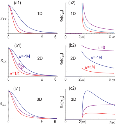
The quantum metric is shown as a function of $k$ in Fig.1(a1). The real part of the optical conductivity (14) is obtained as

\text{Re}\left[\sigma_{xx}\right]=\frac{2\pi e^{2}}{\hbar\left(\hbar\omega/2\right)^{2}}\frac{1}{k_{0}}\frac{\left(m-uk_{0}^{2}\right)^{2}}{\left|v^{2}+2u\left(m+uk_{0}^{2}\right)\right|}.

(23)

The optical conductivity is shown as a function of $\omega$ in Fig.1(a2). At the band-edge frequency $\hbar\omega=2\left|m\right|$ , we have $k_{0}=0$ . Hence, the optical conductivity at the band-edge frequency diverges

\text{Re}\left[\sigma_{xx}\left(\frac{2\left|m\right|}{\hbar}\right)\right]\propto\lim_{k_{0}\rightarrow 0}\frac{1}{k_{0}}=\infty,

(24)

as shown in Fig.1(a2).

Refer to caption — Figure 1: Dirac model. (a1), (b1) and (c1) Quantum metric as a function of $k$ . (a2), (b2) and (c2) Optical conductivity $\text{Re}\left[\sigma_{xx}\right]$ as a function of $\hbar\omega$ . (a1) and (a2) One dimension. (b1) and (b2) Two dimensions. (c1) and (c2) Three dimensions. Red curves indicate $u=t/4$ , purple curves indicate $u=0$ , and blue curves indicate $u=-t/4$ . We have set $m=t$ and $v=t$ .

III.2 Two-dimensional model

In the two-dimensional Dirac Hamiltonian, the quantum metric (11) is simply given by

g_{xx}\left(k\right)=\int_{0}^{\pi}g_{xx}\left(\mathbf{k}\right)d\theta=\frac{\pi v^{2}}{E^{2}}\left(1-\frac{k^{2}}{2}\frac{4mu+v^{2}}{E^{2}}\right).

(25)

The quantum metric as a function of $k$ is shown in Fig.1(b1). The real part of the optical conductivity is obtained as

\text{Re}\left[\sigma_{xx}\left(\omega\right)\right]=\frac{e^{2}\pi^{2}v^{2}}{\hbar\left(\hbar\omega/2\right)^{2}}\frac{\left(vk_{0}\right)^{2}+2\left(m^{2}+u^{2}k_{0}^{4}\right)}{\left|v^{2}+2u\left(m+uk_{0}^{2}\right)\right|}.

(26)

The optical conductivity (14) is shown as a function of $\omega$ in Fig.1(b2). At the band-edge frequency $\hbar\omega=2\left|m\right|$ , we have $k_{0}=0$ . It is given by

\text{Re}\left[\sigma_{xx}\left(\frac{2\left|m\right|}{\hbar}\right)\right]=\frac{e^{2}\pi^{2}v^{2}}{\hbar\left(\hbar\omega/2\right)^{2}}\frac{2m^{2}}{\left|v^{2}+2um\right|},

(27)

which is consistent with the previous study[3] in the case of $u=1$ .

III.3 Three-dimensional model

In the three-dimensional Dirac Hamiltonian, the quantum metric (11) is simply given by

	$\displaystyle g_{xx}\left(k\right)$	$\displaystyle=\int_{0}^{\pi}\sin\theta d\theta g_{xx}\left(\mathbf{k}\right)\int_{0}^{2\pi}d\phi$
		$\displaystyle=4\pi\frac{v^{2}}{E^{2}}\left(1-\frac{k^{2}}{3}\frac{4mu+v^{2}}{E^{2}}\right).$		(28)

The quantum metric as a function of $k$ is shown in Fig.1(c1). The real part of the optical conductivity (14) is obtained as

	$\displaystyle\text{Re}\left[\sigma_{xx}\left(\omega\right)\right]=$	$\displaystyle\pi e^{2}\omega k_{0}\frac{4\pi\frac{v^{2}}{E^{2}}\left(1-k_{0}^{2}\frac{4mu+v^{2}}{3E^{2}}\right)E\left(k_{0}\right)}{\left\|v^{2}+2u\left(m+uk_{0}^{2}\right)\right\|}$
	$\displaystyle=$	$\displaystyle\frac{8\pi^{2}e^{2}v^{2}k_{0}}{3\hbar\left(\hbar\omega/2\right)^{2}}\frac{2v^{2}k_{0}^{2}+3m^{2}+2muk_{0}^{2}+3u^{2}k_{0}^{4}}{\left\|v^{2}+2u\left(m+uk_{0}^{2}\right)\right\|}.$		(29)

The optical conductivity (14) is shown as a function of $\omega$ in Fig.1(c2). The optical conductivity is zero at the band-edge frequency,

\text{Re}\left[\sigma_{xx}\left(\frac{2\left|m\right|}{\hbar}\right)\right]=0

(30)

for $N$ dimensions with $N\geq 3$ .

IV Dirac model without parabolic mass

We study the Dirac Hamiltonian (5) with $u=0$ . The quantum metric is simply given by

g_{xx}\left(\mathbf{k}\right)=\frac{2^{N-3}v^{2}}{E^{2}}\left(1-k_{x}^{2}\frac{v^{2}}{E^{2}}\right),

(31)

and

g_{xx}\left(k\right)=\frac{2^{N-3}v^{2}N\pi^{N/2}}{E^{2}\Gamma\left(\frac{N}{2}+1\right)}\left(1-\frac{v^{2}k^{2}}{NE^{2}}\right).

(32)

They are shown by purple curves in Fig.1(a1), (b1) and (c1).

The real part of the optical conductivity is obtained as

	$\displaystyle\text{Re}\left[\sigma_{xx}\left(\omega\right)\right]$
	$\displaystyle=\frac{2^{N-2}v^{2}Ne^{2}\pi^{N/2+1}\xi_{N}}{\hbar\Gamma\left(\frac{N}{2}+1\right)}\left(1-\frac{v^{2}k_{0}^{2}}{N\left(\frac{\hbar\omega}{2}\right)^{2}}\right)k_{0}^{N-2},$		(33)

where we used the relation

2\partial_{k}E\left(k\right)=2k\frac{v^{2}}{E\left(k\right)}.

(34)

The momentum (15) is singular at $u=0$ . However, we may solve (16) by setting $u=0$ to find that

k_{0}=\frac{\sqrt{\left(\hbar\omega/2\right)^{2}-m^{2}}}{v}.

(35)

By substituting this for $k_{0}$ in Eq.(33), we obtain

	$\displaystyle\text{Re}\left[\sigma_{xx}\left(\omega\right)\right]$	$\displaystyle=\frac{2^{N-2}e^{2}\pi^{N/2+1}\xi_{N}}{\hbar\Gamma\left(\frac{N}{2}+1\right)v^{N-4}\left(\frac{\hbar\omega}{2}\right)^{2}}$
		$\displaystyle\!\!\!\!\times\left(\left(N-1\right)\left(\frac{\hbar\omega}{2}\right)^{2}+m^{2}\right)\left(\left(\hbar\omega/2\right)^{2}-m^{2}\right)^{N/2-1}.$		(36)

It does not depend on the sign of $m$ in contrast to the case of $u\neq 0$ as in Eq.(14). It is shown by purple curves in Fig.1(a2), (b2) and (c2).

V Tight-binding models on the hypercubic lattice

Next, we study the $N$ -dimensional tight-binding model on the hypercubic lattice, where the Dirac vector is given by[46, 43]

d_{0}=m_{0}-t\sum_{j=1}^{N}\cos k_{j},\quad d_{j}=v\sin k_{j},

(37)

where $1\leq j\leq N$ and $m_{0}$ is the model parameter. In the vicinity of the $\Gamma$ point, we have

m=m_{0}-Nt,\qquad u=t/2.

(38)

We explicitly discuss several models in what follows.

V.1 Kitaev model

We study the tight-binding model in one dimensional chain,

H=d_{0}\sigma_{x}+d_{x}\sigma_{y},

(39)

where the Dirac vector is given by

d_{0}=m_{0}-t\cos k,\quad d_{x}=v\sin k,

(40)

and $\sigma_{j}$ is the Pauli matrix. A typical model is the Kitaev $p$ -wave topological superconductor model[47].

The quantum metric is given by

g_{xx}\left(k\right)=\frac{v^{2}\left(t-m_{0}\cos k\right)^{2}}{4E\left(k\right)^{4}}.

(41)

The optical conductivity is calculated as

\text{Re}\left[\sigma_{xx}\left(\omega\right)\right]=\frac{\pi e^{2}v^{2}\left(t-m_{0}\cos k_{0}\right)^{2}}{2\hbar\left(\frac{\hbar\omega}{2}\right)^{2}\left(m_{0}t+\left(v^{2}-t^{2}\right)\cos k_{0}\right)\sin k_{0}},

(42)

where we have used

2\partial_{k}E\left(k\right)=2\frac{\left(m_{0}t+\left(v^{2}-t^{2}\right)\cos k\right)\sin k}{E\left(k\right)}

(43)

with

k_{0}=\arccos\frac{2m_{0}t-\sqrt{4v^{2}\left(m_{0}^{2}-t^{2}+v^{2}\right)+\left(t^{2}-v^{2}\right)\hbar\omega}}{2\left(t^{2}-v^{2}\right)}.

(44)

V.2 SSH model

In the SSH model[35], we have $v=t$ in Eq.(40). In this case, the momentum (44) is singular. However, we may solve (16) by setting $v=t$ to find that

k_{0}=\arccos\frac{\left(m_{0}^{2}+t^{2}\right)-\left(\frac{\hbar\omega}{2}\right)^{2}}{2m_{0}t}.

(45)

By substituting this for $k_{0}$ in Eq.(14), the optical conductivity is simplified as

\text{Re}\left[\sigma_{xx}\left(\omega\right)\right]=\frac{\pi e^{2}}{4\hbar\left(\frac{\hbar\omega}{2}\right)^{2}}\frac{\left(t^{2}-m_{0}^{2}+\left(\frac{\hbar\omega}{2}\right)^{2}\right)^{2}}{\sqrt{\left(2m_{0}t\right)^{2}-\left(\left(m_{0}^{2}+t^{2}\right)-\left(\frac{\hbar\omega}{2}\right)^{2}\right)^{2}}}.

(46)

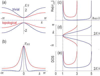
We study two typical cases, $m_{0}=0.5t$ and $m_{0}=1.5t$ , where the system is topological and trivial, respectively.

We show the energy spectrum in Fig.2(a), where the gap is given by $2\left|m_{0}-t\right|$ . The quantum metric is shown in Fig.2(b). The optical conductivity $\text{Re}\left[\sigma_{xx}\left(\omega\right)\right]$ is shown in Fig.2(c). It diverges at $\hbar\omega=2\left|m_{0}-t\right|$ , which is consistent with the Dirac model as shown in Fig.1(a2). In addition, it diverges at $2\left|m_{0}+t\right|$ .

We explain the structure of the optical conductivity in Fig.2(c) as follows. We show Fig.2(d) which is identical to the energy spectrum Fig.2(a) except for the orientation and the scale. The band-edge frequency in the optical conductivity coincides with the band gap $2\left|m_{0}-t\right|$ of the energy spectrum, and the sharp peak in the optical conductivity emerges when the the gap energy $2E$ becomes flat with respect to $k$ in Fig.2(d). We also show the density of states (DOS) in Fig.2(e), where the sharp peak in the optical conductivity is found to be due to the van-Hove singularity.

V.3 QWZ model

As a typical example of the Chern insulator on square lattice, we study the QWZ model[36],

H=\left[m_{0}-t\left(\cos k_{x}+\cos k_{y}\right)\right]\sigma_{z}+v\left(\sigma_{x}\sin k_{x}+\sigma_{y}\sin k_{y}\right),

(47)

where the Dirac vector is given by

	$\displaystyle d_{0}$	$\displaystyle=m_{0}-t\left(\cos k_{x}+\cos k_{y}\right),$
	$\displaystyle d_{x}$	$\displaystyle=v\sin k_{x},\quad d_{y}=v\sin k_{y}.$		(48)

The Dirac vector is obtained as

d_{0}=m_{0}+\xi t+\frac{\zeta_{x}k_{x}^{2}+\zeta_{y}k_{y}^{2}}{2}t,\quad d_{x}=v\eta_{x}k_{x},\quad d_{y}=v\eta_{y}k_{y},

(49)

where $\eta_{x}=1$ , $\eta_{y}=1$ , $\xi=-2$ , $\zeta_{x}=1$ and $\zeta_{y}=1$ at the $\Gamma$ point; $\eta_{x}=-1$ , $\eta_{y}=-1$ , $\xi=2$ , $\zeta_{x}=-1$ and $\zeta_{y}=-1$ at the $M$ point; $\eta_{x}=1$ , $\eta_{y}=-1$ , $\xi=0$ , $\zeta_{x}=-1$ and $\zeta_{y}=1$ at the $X$ point; $\eta_{x}=-1$ , $\eta_{y}=1$ , $\xi=0$ , $\zeta_{x}=1$ and $\zeta_{y}=-1$ at the $Y$ point.

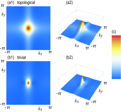
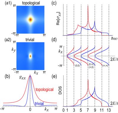
We consider two typical cases, $m_{0}=\left(2-\alpha\right)t$ and $m_{0}=\left(2+\alpha\right)t$ with $0<\alpha<1$ , where the band gap is present at the $\Gamma$ point with the gap $2\alpha t$ , which are identical between the two cases. The system is topological in the case of $m_{0}=\left(2-\alpha\right)t$ , while it is trivial in the case of $m_{0}=\left(2+\alpha\right)t$ . The quantum metric is shown in Fig.3 for $\alpha=0.5$ . The optical conductivity is shown in Fig.4(a1). The optical conductivity is drastically different between the two phases although the band gaps are identical. It is understood as follows. We assume $v=t$ for simplicity.

The optical conductivity at the band-edge frequency $\hbar\omega=2\left|m\right|$ is proportional to

\frac{2m^{2}}{\left|v^{2}+2um\right|}=\frac{2\left(-\alpha t\right)^{2}}{\left|t^{2}-\alpha t^{2}\right|}=\frac{2\alpha^{2}}{\left|1-\alpha\right|}

(50)

in the case $m_{0}=\left(2-\alpha\right)t$ , and

\frac{2m^{2}}{\left|v^{2}+2um\right|}=\frac{2\left(\alpha t\right)^{2}}{\left|t^{2}+\alpha t^{2}\right|}=\frac{2\alpha^{2}}{\left|1+\alpha\right|}

(51)

in the case $m_{0}=\left(2+\alpha\right)t$ . The ratio is

\frac{1+\alpha}{1-\alpha}=3

(52)

for $\alpha=0.5$ , which is significantly large.

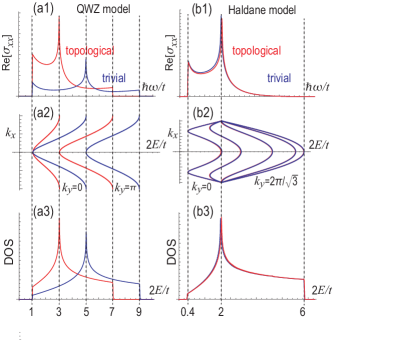
We explain the structure of the optical conductivity in Fig.4(a1) as in the case of the SSH model. We show a figure which is identical to the energy spectrum except for the orientation and the scale in Fig.4(a2). The band-edge frequency in the optical conductivity coincides with the band gap $2\left|m_{0}-2t\right|$ of the energy spectrum, and the sharp peak in the optical conductivity emerges when the the gap energy $2E$ becomes flat with respect to $k_{x}$ in Fig.4(a2). We also show the density of states (DOS) in Fig.4(a3), where the sharp peak in the optical conductivity is due to the van-Hove singularity.

V.4 Haldane model

Next, we study the Haldane model on the honeycomb lattice[25],

H=d_{0}\sigma_{z}+d_{x}\sigma_{x}+d_{y}\sigma_{y},

(53)

where the Dirac vector is given by

$\displaystyle d_{0}$	$\displaystyle=m_{0}+\frac{\lambda}{3\sqrt{3}}\left(\sin k_{x}-\sum_{\pm}\sin\frac{k_{x}\pm\sqrt{3}k_{y}}{2}\right),$
$\displaystyle d_{x}$	$\displaystyle=t\left(\cos\frac{k_{y}}{\sqrt{3}}+2\cos\frac{2k_{y}}{\sqrt{3}}\cos\frac{k_{x}}{2}\right),$
$\displaystyle d_{y}$	$\displaystyle=t\left(-\sin\frac{k_{y}}{\sqrt{3}}+2\sin\frac{2k_{y}}{\sqrt{3}}\cos\frac{k_{x}}{2}\right).$	(54)

There exist Dirac cones at the $K$ point ( $\eta=1$ ) and the $K^{\prime}$ point ( $\eta=-1$ ), where $(k_{x},k_{y})=(4\pi\eta/3,0)$ . We define the momentum $k_{x}^{\prime}=k_{x}-4\pi\eta/3$ measured from the $K$ or $K^{\prime}$ point, and we replace $k$ in Eq.(8) with $k^{\prime}$ . The Dirac mass $m$ , the velocity $v$ and parabolic coefficient $u$ are given by

m=m_{0}-\eta\lambda,\quad v=\sqrt{3}t/2,\quad u=\eta\lambda/4.

(55)

We study two cases, $(m_{0},\lambda)=\left(\alpha t,0\right)$ and $(m_{0},\lambda)=\left(0,\alpha t\right)$ , where the gaps are identical. The system is trivial in the case of $(m_{0},\lambda)=\left(\alpha t,0\right)$ , while it is topological in the case of $(m_{0},\lambda)=\left(0,\alpha t\right)$ . The quantum metric is shown in Fig.5 for $\alpha=0.2$ . The quantum metrics are almost identical between the two cases. The optical conductivity is shown in Fig.4(b1). The difference is tiny between the two cases. It is understood as follows. The optical conductivity at the band-edge frequency is

\frac{2m^{2}}{\left|v^{2}+2um\right|}=\frac{2\left(\alpha t\right)^{2}}{\left|\left(\frac{\sqrt{3}t}{2}\right)^{2}\right|}=\frac{2\alpha^{2}}{3/4}

(56)

in the case $(m_{0},\lambda)=\left(\alpha t,0\right)$ , while it is

\frac{2m^{2}}{\left|v^{2}+2um\right|}=\frac{2\left(\alpha t\right)^{2}}{\left|\left(\frac{\sqrt{3}t}{2}\right)^{2}+2\frac{\alpha t}{4}\alpha t\right|}=\frac{2\alpha^{2}}{3/4+\alpha^{2}/2}

(57)

in the case $(m_{0},\lambda)=\left(0,\alpha t\right)$ . The ratio is

\frac{3/4+\alpha^{2}/2}{3/4}=1.027

(58)

for $\alpha=0.2$ , which is very tiny.

The structure of the optical conductivity in Fig.4(b1) is understood as in the case of the QWZ model. Namely, the band-edge frequency in the optical conductivity coincides with the band gap of the energy spectrum as in Fig.4(b2), and the sharp peak in the optical conductivity is due to the van-Hove singularity in the DOS in Fig.4(b3).

V.5 Three-dimensional lattice Dirac model

Finally, we study the tight-binding model on the cubic lattice, whose Hamiltonian is given by[48, 49]

	$\displaystyle H$	$\displaystyle=\left[m_{0}-t\left(\cos k_{x}+\cos k_{y}+\cos k_{z}\right)\right]\sigma_{z}$
		$\displaystyle+v\left(\sigma_{x}\sin k_{x}+\sigma_{y}\sin k_{y}+\sigma_{z}\sin k_{z}\right).$		(59)

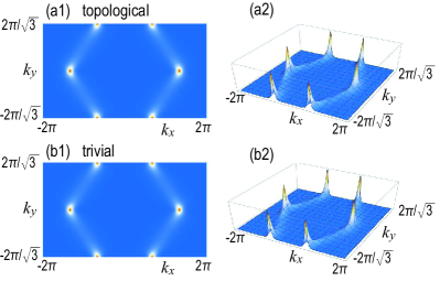
It describes three-dimensional topological insulators[48, 49] such as Bi₂Se₃ and Bi₂Te₃. The quantum metric is shown in Fig.6(a1), (a2) and (b). The optical conductivity is shown in Fig.6(c). The band-edge frequency of the optical conductivity coincides with the band structure as in Fig.6(d). The optical conductivity at the band-edge frequency is zero, which is consistent with the Dirac model as shown in Fig.1(c2). The sharp peak in the optical conductivity is due to the van-Hove singularity of the DOS as in Fig.6(e).

VI Conclusion

We have analytically determined the quantum metric and the optical conductivity in the Dirac model with parabolic mass term in arbitrary dimensions, and revealed that the parabolic dispersion of the Dirac mass term quite affects the optical absorption. In addition, we have shown that the optical absorption at the band-edge frequency exhibits a distinct behavior depending on the dimension. We have studied two typical Chern insulators, i.e., the QWZ model and the Haldane model. By comparing the topological and trivial phases with the same gap, the optical absorption is significantly different in these two phases in the QWZ model but not in the Haldane model.

This work is supported by CREST, JST (Grants No. JPMJCR20T2) and Grants-in-Aid for Scientific Research from MEXT KAKENHI (Grant No. 23H00171).

Appendix A Quantum geometric tensor and quantum metric

We review the relation between the optical conductivity and the quantum metric[3]. The quantum distance is defined by[23, 24]

	$\displaystyle ds^{2}$	$\displaystyle=\sum_{nm}\left\|\left\|\psi_{n}\left(\mathbf{k}+\delta\mathbf{k}\right)-\psi_{m}\left(\mathbf{k}\right)\right\|\right\|^{2}$
		$\displaystyle=\sum_{nm}\left\langle\psi_{n}\left(\mathbf{k}+\delta\mathbf{k}\right)-\psi_{m}\left(\mathbf{k}\right)\|\psi_{n}\left(\mathbf{k}+\delta\mathbf{k}\right)-\psi_{m}\left(\mathbf{k}\right)\right\rangle.$		(60)

Up to the second order, it is expanded as

	$\displaystyle ds^{2}$	$\displaystyle=\sum_{nm}\sum_{\mu\nu}\left\langle\partial_{k_{\mu}}\psi_{n}\left(\mathbf{k}\right)dk_{\mu}\left\|\partial_{k_{\nu}}\psi_{m}\left(\mathbf{k}\right)dk_{\nu}\right\rangle\right.dk_{\mu}dk_{\nu}$
		$\displaystyle=\sum_{nm}\sum_{\mu\nu}\mathcal{Q}_{\mu\nu}^{nm}\left(\mathbf{k}\right)dk_{\mu}dk_{\nu},$		(61)

where $Q_{\mu\nu}^{nm}\left(\mathbf{k}\right)$ is the quantum geometric tensor, and given by[24]

\mathcal{Q}_{\mu\nu}^{nm}\left(\mathbf{k}\right)=\left\langle\partial_{k_{\mu}}\psi_{n}\left(\mathbf{k}\right)\right|1-P\left(\mathbf{k}\right)\left|\partial_{k_{\nu}}\psi_{m}\left(\mathbf{k}\right)\right\rangle,

(62)

with the projection operator

P\left(\mathbf{k}\right)\equiv\sum_{n}\left|\psi_{n}\left(\mathbf{k}\right)\right\rangle\left\langle\psi_{n}\left(\mathbf{k}\right)\right|.

(63)

The quantum geometric tensor is decomposed as

\mathcal{Q}_{\mu\nu}^{nm}\left(\mathbf{k}\right)=g_{\mu\nu}^{nm}-\frac{i}{2}F_{\mu\nu}^{nm},

(64)

where

g_{\mu\nu}^{nm}\equiv\frac{\mathcal{Q}_{\mu\nu}^{nm}+\mathcal{Q}_{\mu\nu}^{nm\dagger}}{2}=\text{Re}\left[\mathcal{Q}_{\mu\nu}^{nm}\right]

(65)

is the quantum metric, and

F_{\mu\nu}^{nm}\equiv i\left(\mathcal{Q}_{\mu\nu}^{nm}-\mathcal{Q}_{\mu\nu}^{nm\dagger}\right)=\text{Im}\left[\mathcal{Q}_{\mu\nu}^{nm}\right]

(66)

is the non-Abelian Berry curvature.

Appendix B Quantum metric and optical conductivity

The optical conductivity is calculated based on the Kubo formula as

	$\displaystyle\sigma_{\mu\nu}\left(\omega\right)$
	$\displaystyle=\frac{e^{2}}{\hbar}\int d\mathbf{k}\sum_{n,m}\left(f_{n}\left(\mathbf{k}\right)-f_{m}\left(\mathbf{k}\right)\right)\frac{\varepsilon_{mn}\left(\mathbf{k}\right)A_{nm}^{\mu}\left(\mathbf{k}\right)A_{nm}^{\nu}\left(\mathbf{k}\right)}{\varepsilon_{n}\left(\mathbf{k}\right)-\varepsilon_{m}\left(\mathbf{k}\right)+\hbar\omega+i\eta}$
	$\displaystyle=\pi\omega e^{2}\int d\mathbf{k}\sum_{n,m}\left(f_{n}\left(\mathbf{k}\right)-f_{m}\left(\mathbf{k}\right)\right)A_{nm}^{\mu}\left(\mathbf{k}\right)A_{nm}^{\nu}\left(\mathbf{k}\right)$
	$\displaystyle\qquad\qquad\times\delta\left(\varepsilon_{n}\left(\mathbf{k}\right)-\varepsilon_{m}\left(\mathbf{k}\right)-\hbar\omega\right),$		(67)

where $A_{nm}^{\alpha}$ is the inter-band Berry connection defined as

A_{nm}^{\mu}\left(\mathbf{k}\right)=i\left\langle\psi_{n}\left(\mathbf{k}\right)\right|\partial_{k_{\mu}}\left|\psi_{m}\left(\mathbf{k}\right)\right\rangle,

(68)

while $f_{n}\left(\mathbf{k}\right)$ is the Fermi distribution function and $\varepsilon_{n}\left(\mathbf{k}\right)$ is the band dispersion and $\eta$ is an infinitesimal real number.

Here, we have

	$\displaystyle\sum_{nm}A_{nm}^{\mu}\left(\mathbf{k}\right)A_{mn}^{\nu}\left(\mathbf{k}\right)$
	$\displaystyle=-\sum_{nm}\left\langle\psi_{n}\left(\mathbf{k}\right)\right\|\partial_{k_{\mu}}\left\|\psi_{m}\left(\mathbf{k}\right)\right\rangle\left\langle\psi_{m}\left(\mathbf{k}\right)\right\|\partial_{k_{\nu}}\left\|\psi_{n}\left(\mathbf{k}\right)\right\rangle$
	$\displaystyle=\sum_{nm}\left\langle\partial_{k_{\mu}}\psi_{n}\left(\mathbf{k}\right)\left\|\psi_{m}\left(\mathbf{k}\right)\right\rangle\right.\left\langle\psi_{m}\left(\mathbf{k}\right)\left\|\partial_{k_{\nu}}\psi_{n}\left(\mathbf{k}\right)\right\rangle\right.$
	$\displaystyle=\sum_{nm}\left\langle\partial_{k_{\mu}}\psi_{n}\left(\mathbf{k}\right)\right\|P_{m}\left\|\partial_{k_{\nu}}\psi_{n}\left(\mathbf{k}\right)\right\rangle$
	$\displaystyle=\sum_{nm}\left\langle\partial_{k_{\mu}}\psi_{n}\left(\mathbf{k}\right)\right\|\left(1-P_{n}\right)-\left(1-P_{n}-P_{m}\right)\left\|\partial_{k_{\nu}}\psi_{n}\left(\mathbf{k}\right)\right\rangle$
	$\displaystyle=\mathcal{Q}_{\mu\nu}^{nn}\left(\mathbf{k}\right),$		(69)

where we have used the fact that the complete sum of the quantum metric over the valence and conduction bands is zero, or

\left\langle\partial_{k_{\mu}}\psi_{n}\left(\mathbf{k}\right)\right|\left(1-P_{n}-P_{m}\right)\left|\partial_{k_{\nu}}\psi_{n}\left(\mathbf{k}\right)\right\rangle=0.

(70)

Then, taking the real part, we have

\sum_{nm}\text{Re}\left[A_{nm}^{\mu}\left(\mathbf{k}\right)A_{mn}^{\nu}\left(\mathbf{k}\right)\right]=\sum_{n}g_{\mu\nu}^{nn}=g_{\mu\nu},

(71)

where we have defined

g_{\mu\nu}=\sum_{n}g_{\mu\nu}^{nn}

(72)

and the real part of the optical conductivity is calculated as

	$\displaystyle\text{Re}[\sigma_{xx}\left(\omega\right)]$
	$\displaystyle=\pi\omega e^{2}\int d\mathbf{k}\sum_{n,m}\left(f_{n}\left(\mathbf{k}\right)-f_{m}\left(\mathbf{k}\right)\right)$
	$\displaystyle\qquad\qquad\times\text{Re}\left[A_{nm}^{\alpha}\left(\mathbf{k}\right)A_{nm}^{\beta}\left(\mathbf{k}\right)\right]\delta\left(\varepsilon_{n}\left(\mathbf{k}\right)-\varepsilon_{m}\left(\mathbf{k}\right)-\hbar\omega\right)$
	$\displaystyle=\pi\omega e^{2}\int d\mathbf{k}\sum_{n,m}\left(f_{n}\left(\mathbf{k}\right)-f_{m}\left(\mathbf{k}\right)\right)$
	$\displaystyle\qquad\qquad\times\text{Tr}\left[g_{xx}\right]\delta\left(\varepsilon_{n}\left(\mathbf{k}\right)-\varepsilon_{m}\left(\mathbf{k}\right)-\hbar\omega\right).$		(73)

This is Eq.(7) in the main text.

Appendix C Detailed derivation of quantum metric

We obtain

	$\displaystyle\sum_{j}\left(\partial_{k_{x}}n_{j}\right)^{2}$
	$\displaystyle=\left(\frac{2uk_{x}}{E}-\frac{m+uk^{2}}{E^{3}}k_{x}\mathcal{E}\right)^{2}+\left(\frac{v}{E}-\frac{vk_{x}^{2}}{E^{3}}\mathcal{E}\right)^{2}$
	$\displaystyle+\sum_{j=2}^{N}\left(-\frac{vk_{j}k_{x}}{E^{3}}\mathcal{E}\right)^{2},$		(74)

where we have introduced

\mathcal{E=}v^{2}+2mu+2u^{2}k^{2}.

(75)

We further obtain

	$\displaystyle\sum_{j}\left(\partial_{k_{x}}n_{j}\right)^{2}$	(76)
$\displaystyle=$	$\displaystyle\frac{1}{E^{6}}[\left(2uk_{x}E^{2}\right)^{2}+\left(m+uk^{2}\right)^{2}k_{x}^{2}\mathcal{E}^{2}$
	$\displaystyle-4uk_{x}E^{2}\left(m+uk^{2}\right)k_{x}\mathcal{E}+\left(vE^{2}\right)^{2}$
	$\displaystyle+\left(vk_{x}^{2}\mathcal{E}\right)^{2}-2vE^{2}vk_{x}^{2}\mathcal{E+}\sum_{j=2}^{N}\left(vk_{j}k_{x}\mathcal{E}\right)^{2}$
$\displaystyle=$	$\displaystyle\frac{1}{E^{6}}\left(vk_{x}\mathcal{E}\right)^{2}\sum_{j=1}^{N}k_{j}^{2}+\frac{\left(2uk_{x}\right)^{2}+v^{2}}{E^{2}}$
	$\displaystyle-\frac{2\mathcal{E}^{2}k_{x}^{2}}{E^{4}}+\frac{\left(m+uk^{2}\right)^{2}k_{x}^{2}\mathcal{E}^{2}}{E^{6}}$
$\displaystyle=$	$\displaystyle\frac{k_{x}^{2}\mathcal{E}^{2}}{E^{6}}\left(v^{2}k^{2}+\left(m+uk^{2}\right)^{2}\right)+\frac{\left(2uk_{x}\right)^{2}+v^{2}}{E^{2}}-\frac{2\mathcal{E}^{2}k_{x}^{2}}{E^{4}}$
$\displaystyle=$	$\displaystyle\frac{k_{x}^{2}\mathcal{E}^{2}}{E^{6}}E^{2}+\frac{\left(2uk_{x}\right)^{2}+v^{2}}{E^{2}}-\frac{2\mathcal{E}^{2}k_{x}^{2}}{E^{4}}$
$\displaystyle=$	$\displaystyle-\frac{k_{x}^{2}\mathcal{E}^{2}}{E^{4}}+\frac{\left(2uk_{x}\right)^{2}+v^{2}}{E^{2}}$
$\displaystyle=$	$\displaystyle\frac{v^{2}}{E^{2}}\left(1-k_{x}^{2}\frac{4mu+v^{2}}{E^{2}}\right).$

Hence, the quantum metric is given by

g_{xx}\left(\mathbf{k}\right)=\frac{2^{N-3}v^{2}}{E^{2}}\left(1-k_{x}^{2}\frac{4mu+v^{2}}{E^{2}}\right).

(77)

This is Eq.(10) in the main text.

Appendix D ( $N$ -1)-sphere

We summarize the ( $N$ -1)-sphere coordinate. The momenta are parametrized as

$\displaystyle k_{1}$	$\displaystyle=k\cos\theta_{1},$
$\displaystyle k_{2}$	$\displaystyle=k\sin\theta_{1}\cos\theta_{2}$
$\displaystyle k_{3}$	$\displaystyle=k\sin\theta_{1}\sin\theta_{2}\cos\theta_{3}$
$\displaystyle k_{4}$	$\displaystyle=k\sin\theta_{1}\sin\theta_{2}\sin\theta_{3}\cos\theta_{4}$
	$\displaystyle\cdots$
$\displaystyle k_{N}$	$\displaystyle=k\sin\theta_{1}\sin\theta_{2}\sin\theta_{3}\cdots\sin\theta_{N-1},$	(78)

where $0\leq k\leq\infty$ , $0\leq\theta_{j}\leq\pi$ for $1\leq j\leq N-2$ and $0\leq\theta_{N-1}\leq 2\pi$ . The Jacobian is given by

J=k^{N-1}\sin^{N-2}\theta_{1}\sin_{2}^{N-3}\theta\cdots\sin\theta_{N-2}dkd\theta_{1}d\theta_{2}\cdots d\theta_{N-1}.

(79)

The area of the ( $N$ -1)-sphere is given by

\int_{0}^{\pi}d\theta_{1}\int_{0}^{\pi}d\theta_{2}\cdots\int_{0}^{\pi}d\theta_{N-2}\int_{0}^{2\pi}d\theta_{N-1}J=\frac{N\pi^{N/2}}{\Gamma\left(\frac{N}{2}+1\right)}.

(80)

It is $2$ for $N=1$ , $2\pi$ for $N=2$ and $4\pi$ for $N=3$ . On the other hand

	$\displaystyle\int_{0}^{\pi}d\theta_{1}\int_{0}^{\pi}d\theta_{2}\cdots\int_{0}^{\pi}d\theta_{N-2}\int_{0}^{2\pi}d\theta_{N-1}J\frac{k_{x}^{2}}{k^{2}}$
	$\displaystyle=\int_{0}^{\pi}d\theta_{1}\int_{0}^{\pi}d\theta_{2}\cdots\int_{0}^{\pi}d\theta_{N-2}\int_{0}^{2\pi}d\theta_{N-1}J\cos^{2}\theta_{1}$
	$\displaystyle=\frac{N\pi^{N/2}\Gamma\left(\frac{N}{2}\right)}{2\Gamma\left(\frac{N}{2}+1\right)^{2}}=\frac{\pi^{N/2}}{\Gamma\left(\frac{N}{2}+1\right)}.$		(81)

It is $2$ for $N=1$ , $\pi$ for $N=2$ and $4\pi/3$ for $N=3$ . They are used in the integration of $g\left(\mathbf{k}\right)$ to derive $g\left(k\right)$ in Eq.(11).

References

[1] Shunji Matsuura and Shinsei Ryu, Momentum space metric, nonlocal operator, and topological insulators, Phys. Rev. B 82, 245113 (2010)
[2] Tomoki Ozawa and Bruno Mera, Relations between topology and the quantum metric for Chern insulators, Phys. Rev. B 104, 045103 (2021)
[3] Yugo Onishi and Liang Fu, Fundamental Bound on Topological Gap, Phys. Rev. X 14, 011052 (2024)
[4] A. M. Cook, B. M. Fregoso, F. de Juan, S. Coh, J. E. Moore, Design principles for shift current photovoltaics, Nature Communications 8, 14176 (2017).
[5] F. de Juan, A. G. Grushin, T. Morimoto, J. E. Moore, Quantized circular photogalvanic effect in Weyl semimetals, Nature Communications 8, 15995 (2017).
[6] J. Ahn, G.-Y. Guo, N. Nagaosa, Low-Frequency Divergence and Quantum Geometry of the Bulk Photovoltaic Effect in Topological Semimetals, Phys. Rev. X 10, 041041 (2020).
[7] T. Holder, D. Kaplan, B. Yan, Consequences of time-reversal-symmetry breaking in the light-matter interaction: Berry curvature, quantum metric, and diabatic motion, Phys. Rev. Res. 2, 033100 (2020).
[8] P. Bhalla, K. Das, D. Culcer, A. Agarwal, Resonant Second-Harmonic Generation as a Probe of Quantum Geometry, Phys. Rev. Lett. 129, 227401 (2022)
[9] J. Ahn, G.-Y. Guo, N. Nagaosa, A. Vishwanath, Riemannian geometry of resonant optical responses, Nature Physics 18, 290 (2022)
[10] Barun Ghosh, Yugo Onishi, Su-Yang Xu, Hsin Lin, Liang Fu and Arun Bansil, Probing quantum geometry through optical conductivity and magnetic circular dichroism, arXiv:2401.09689
[11] I. Sodemann and L. Fu, Quantum nonlinear Hall effect induced by Berry curvature dipole in time-reversal invariant materials, Phys. Rev. Lett. 115, 216806 (2015).
[12] Q. Ma, et al., Observation of the nonlinear Hall effect under time-reversal-symmetric conditions, Nature 565, 337 (2019)
[13] C. Wang, Y. Gao, and D. Xiao, Intrinsic nonlinear Hall effect in antiferromagnetic tetragonal cumnas, Phys. Rev. Lett. 127, 277201 (2021).
[14] Kamal Das, Shibalik Lahiri, Rhonald Burgos Atencia, Dimitrie Culcer, and Amit Agarwal, Intrinsic nonlinear conductivities induced by the quantum metric, Phys. Rev. B 108, L201405 (2023)
[15] A. Gao, Y.-F. Liu, J.-X. Qiu, B. Ghosh, T.V. Trevisan, Y. Onishi, C. Hu, T. Qian, H.-J. Tien, S.-W. Chen et al., Quantum metric nonlinear Hall effect in a topological antiferromagnetic heterostructure, Science 381, eadf1506 (2023).
[16] N. Wang, D. Kaplan, Z. Zhang, T. Holder, N. Cao, A. Wang, X. Zhou, F. Zhou, Z. Jiang, C. Zhang et al., Quantum metric-induced nonlinear transport in a topological antiferromagnet, Nature (London) 621, 487 (2023).
[17] Daniel Kaplan, Tobias Holder and Binghai Yan, Unification of Nonlinear Anomalous Hall Effect and Nonreciprocal Magnetoresistance in Metals by the Quantum Geometry, Phys. Rev. Lett. 132, 026301 (2024)
[18] Giacomo Sala, et.al., The quantum metric of electrons with spin-momentum locking, arXiv:2407.06659
[19] Yuan Fang, Jennifer Cano, and Sayed Ali Akbar Ghorashi, Quantum Geometry Induced Nonlinear Transport in Altermagnets, Phys. Rev. Lett. 133, 106701 (2024)
[20] Ivo Souza, Tim Wilkens, and Richard M. Martin, Polarization and localization in insulators: Generating function approach, Phys. Rev. B 62, 1666 (2000)
[21] M. V. Berry, Quantal phase factors accompanying adiabatic changes, Proc. R. Soc. A 392, 45 (1984).
[22] M. V. Berry, The quantum phase, five years after, in Geometric Phases in Physics, edited by F. Wilczek and A. Shapere, Advanced Series in Mathematical Physics Vol. 5 (World Scientific, Singapore, 1989), pp. 7–28.
[23] J. P. Provost and G. Vallee, Riemannian structure on manifolds of quantum states, Comm. Math. Phys. 76, 289 (1980).
[24] Yu-Quan Ma, Shu Chen, Heng Fan, and Wu-Ming Liu, Abelian and non-Abelian quantum geometric tensor, Phys. Rev. B 81, 245129 (2010).
[25] F. D. M. Haldane, Model for a Quantum Hall Effect without Landau Levels: Condensed-Matter Realization of the "Parity Anomaly", Phys. Rev. Lett. 61, 2015 (1988)
[26] D. J. Thouless, M. Kohmoto, M. P. Nightingale and M. den Nijs, Phys. Rev. Lett. 49, 405 (1982).
[27] X. Tan, et al., Experimental Measurement of the Quantum Metric Tensor and Related Topological Phase Transition with a Superconducting Qubit, Phys. Rev. Lett. 122, 210401 (2019).
[28] A. Gianfrate, et al., Measurement of the quantum geometric tensor and of the anomalous Hall drift, Nature 578, 381 (2020).
[29] M. Yu, et al., Experimental measurement of the quantum geometric tensor using coupled qubits in diamond, Natl. Sci. Rev. 7, 254 (2020)
[30] J. Ren, et al., Nontrivial band geometry in an optically active system, Nat. Commun. 12, 689 (2021)
[31] Q. Liao, et al., Experimental Measurement of the Divergent Quantum Metric of an Exceptional Point, Phys. Rev. Lett. 127, 107402 (2021)
[32] H. Tian, et al., Evidence for Dirac flat band superconductivity enabled by quantum geometry, Nature 614, 440 (2023).
[33] Chang-Rui Yi, Jinlong Yu, Huan Yuan, Rui-Heng Jiao, Yu-Meng Yang, Xiao Jiang, Jin-Yi Zhang, Shuai Chen, and Jian-Wei, Extracting the quantum geometric tensor of an optical Raman lattice by Bloch-state tomography, Pan Phys. Rev. Research 5, L032016 (2023)
[34] H. B. Nielsen and M. Ninomiya, Absence of neutrinos on a lattice: (I). Proof by homotopy theory, Nuclear Physics B 185, 20 (1981)
[35] W. P. Su, J. R. Schrieffer, and A. J. Heeger, Phys. Rev. Lett. 42, 1698 (1979).
[36] X. L. Qi, Y. S. Wu and S. C. Zhang, Topological quantization of the spin Hall effect in two-dimensional paramagnetic semiconductors. Phys. Rev. B 74, 085308 (2006)
[37] Liang Fu and C. L. Kane, Topological insulators with inversion symmetry, Phys. Rev. B 76, 045302 (2007).
[38] A. P. Schnyder, S. Ryu, A. Furusaki, and A. W. W. Ludwig, Classification of topological insulators and superconductors in three spatial dimensions, Phys. Rev. B 78, 195125 (2008).
[39] S. Ryu, A. P. Schnyder, A. Furusaki, and A. W. W. Ludwig, Topological insulators and superconductors: tenfold way and dimensional hierarchy, New J. Phys. 12, 065010 (2010).
[40] C.-K. Chiu, J. C. Y. Teo, A. P. Schnyder, and S. Ryu, Classification of topological quantum matter with symmetries, Rev. Mod. Phys. 88, 035005 (2016).
[41] R. Resta, The insulating state of matter: a geometrical theory, Eur. Phys. J. B 79, 121 (2011)
[42] G. von Gersdorff and W. Chen, Measurement of topological order based on metric-curvature correspondence, Phys. Rev. B 104, 195133 (2021).
[43] Wei Chen, Quantum geometrical properties of topological materials, arXiv:2406.15145
[44] W. Chen and G. von Gersdorff, Measurement of interaction-dressed Berry curvature and quantum metric in solids by optical absorption, SciPost Phys. Core 5, 040 (2022).
[45] Matheus S. M. de Sousa, Antonio L. Cruz, and Wei Chen, Mapping quantum geometry and quantum phase transitions to real space by a fidelity marker, Phys. Rev. B 107, 205133
[46] W. Chen, Absence of equilibrium edge currents in theoretical models of topological insulators, Phys. Rev. B 101, 195120 (2020)
[47] A. Yu Kitaev, Unpaired Majorana fermions in quantum wires, Phys.-Usp. 44 131 (2001).
[48] H. Zhang, C.-X. Liu, X.-L. Qi, X. Dai, Z. Fang, and S.-C. Zhang, Topological insulators in Bi2Se3, Bi2Te3 and Sb2Te3 with a single Dirac cone on the surface, Nat. Phys. 5, 438 (2009).
[49] C.-X. Liu, X.-L. Qi, H. Zhang, X. Dai, Z. Fang, and S.-C. Zhang, Model Hamiltonian for topological insulators, Phys. Rev. B 82, 045122 (2010).

	$\displaystyle\sum_{nm}A_{nm}^{\mu}\left(\mathbf{k}\right)A_{mn}^{\nu}\left(\mathbf{k}\right)$
	$\displaystyle=-\sum_{nm}\left\langle\psi_{n}\left(\mathbf{k}\right)\right\|\partial_{k_{\mu}}\left\|\psi_{m}\left(\mathbf{k}\right)\right\rangle\left\langle\psi_{m}\left(\mathbf{k}\right)\right\|\partial_{k_{\nu}}\left\|\psi_{n}\left(\mathbf{k}\right)\right\rangle$
	$\displaystyle=\sum_{nm}\left\langle\partial_{k_{\mu}}\psi_{n}\left(\mathbf{k}\right)\left\|\psi_{m}\left(\mathbf{k}\right)\right\rangle\right.\left\langle\psi_{m}\left(\mathbf{k}\right)\left\|\partial_{k_{\nu}}\psi_{n}\left(\mathbf{k}\right)\right\rangle\right.$
	$\displaystyle=\sum_{nm}\left\langle\partial_{k_{\mu}}\psi_{n}\left(\mathbf{k}\right)\right\|P_{m}\left\|\partial_{k_{\nu}}\psi_{n}\left(\mathbf{k}\right)\right\rangle$
	$\displaystyle=\sum_{nm}\left\langle\partial_{k_{\mu}}\psi_{n}\left(\mathbf{k}\right)\right\|\left(1-P_{n}\right)-\left(1-P_{n}-P_{m}\right)\left\|\partial_{k_{\nu}}\psi_{n}\left(\mathbf{k}\right)\right\rangle$
	$\displaystyle=\mathcal{Q}_{\mu\nu}^{nn}\left(\mathbf{k}\right),$		(69)

Analytic approach to quantum metric and optical conductivity in Dirac models with parabolic mass in arbitrary dimensions

Abstract

I Introduction

II Quantum metric and optical absorption

III Dirac model with parabolic mass term

III.1 One-dimensional model

III.2 Two-dimensional model

III.3 Three-dimensional model

IV Dirac model without parabolic mass

V Tight-binding models on the hypercubic lattice

V.1 Kitaev model

V.2 SSH model

V.3 QWZ model

V.4 Haldane model

V.5 Three-dimensional lattice Dirac model

VI Conclusion

Appendix A Quantum geometric tensor and quantum metric

Appendix B Quantum metric and optical conductivity

Appendix C Detailed derivation of quantum metric

Appendix D (NN-1)-sphere

References

Analytic approach to quantum metric and optical conductivity
in Dirac models with parabolic mass in arbitrary dimensions

Appendix D ( $N$ -1)-sphere