Analytical Expressions for Neutrino Oscillation

After adding the brief comment about the vacuum oscillation probability, we are able to explore some limits that can be used in the context of the advancement of Eq. (2). Now, for $L=0$ we obviously get $P_{\alpha\beta}=\delta_{\alpha\beta}$. As $L$ increases, the effects of the larger $\Delta m^{2}_{ij}$ will show up first, and since the mass differences are hierarchical, we may start from the regime where:

$$\frac{\Delta m^{2}_{31}L}{4E}=\frac{\Delta m^{2}_{32}L}{4E}\gtrsim 1~{}~{}~{};~{}~{}~{}\frac{\Delta m^{2}_{21}L}{4E}=0.$$

Then, for a 3-neutrino scenario, the probability is

	$\displaystyle P_{\alpha\beta}=\delta_{\alpha\beta}$	$\displaystyle-$	$\displaystyle 4\left(\sum_{j<3}\Re\left[U^{*}_{\alpha 3}U_{\beta 3}U_{\alpha j}U^{*}_{\beta j}\right]\right)\sin^{2}\left(\frac{\Delta M^{2}L}{4E}\right)$		(8)
		$\displaystyle+$	$\displaystyle 2\left(\sum_{j<3}\Im\left[U^{*}_{\alpha 3}U_{\beta 3}U_{\alpha j}U^{*}_{\beta j}\right]\right)\sin\left(\frac{\Delta M^{2}L}{2E}\right),$

where $\Delta M^{2}=\Delta m^{2}_{31}=\Delta m^{2}_{32}$.

Reactor experiments:

We now want to employ Eq. (8) in experimental scenarios. For instance, in a nuclear reactor, the beta decay of fission products is an abundant source of  $\overline{\nu}_{e}$. Thus, reactor experiments [9], e.g. Double-Chooz, Daya-Bay and Reno, usually study the survival probability of electron anti-neutrinos

	$\displaystyle P_{ee}$	$\displaystyle=$	$\displaystyle 1-4\left(|U_{e3}|^{2}|U_{e1}|^{2}+|U_{e3}|^{2}|U_{e2}|^{2}\right)\sin^{2}\left(\frac{\Delta M^{2}L}{4E}\right)$
		$\displaystyle=$	$\displaystyle 1-4|U_{e3}|^{2}\left(1-|U_{e3}|^{2}\right)\sin^{2}\left(\frac{\Delta M^{2}L}{4E}\right),$

which, replacing the mixing angles given by Eq. (6), it is possible to achieve the familiar form

$$P_{ee}=1-\sin^{2}(2\theta_{13})\sin^{2}\left(\frac{\Delta M^{2}L}{4E}\right).$$

(9)

There are no reactor experiments measuring a non-electronic appearance in an electronic neutrino flux, but the probabilities can be calculated by the same procedure. However, there is a more elegant way to arrive at these probabilities. First, consider the time evolution equation

$$i\frac{d}{dt}\left(\begin{array}[]{c}\nu_{e}\\ \nu_{\mu}\\ \nu_{\tau}\end{array}\right)=H\left(\begin{array}[]{c}\nu_{e}\\ \nu_{\mu}\\ \nu_{\tau}\end{array}\right),$$

which in mass basis, can be written as

$$i\frac{d}{dt}\left(\begin{array}[]{c}\nu_{1}\\ \nu_{2}\\ \nu_{3}\end{array}\right)=\left(\begin{array}[]{ccc}\frac{m_{1}^{2}}{2E}&0&0\\ 0&\frac{m_{2}^{2}}{2E}&0\\ 0&0&\frac{m_{3}^{2}}{2E}\\ \end{array}\right)\left(\begin{array}[]{c}\nu_{1}\\ \nu_{2}\\ \nu_{3}\end{array}\right).$$

To return to flavour basis, we observe that the mixing between mass eingenstates $\nu_{i}$ and flavour eigenstates $\nu_{\alpha}$ is given by $\nu_{\alpha}=U\nu_{i}$. Also, we can decompose the $U$ matrix into its rotational components, and following the notation defined in Eq. (6), we adopt the prescription $U_{ij}\equiv R(\theta_{ij})$, resulting in the following compact parametrization:

$$i\frac{d}{dt}\left(\begin{array}[]{c}\nu_{e}\\ \nu_{\mu}\\ \nu_{\tau}\end{array}\right)=U_{23}U_{13}U_{12}\left(\begin{array}[]{ccc}\frac{m_{1}^{2}}{2E}&0&0\\ 0&\frac{m_{2}^{2}}{2E}&0\\ 0&0&\frac{m_{3}^{2}}{2E}\\ \end{array}\right)U_{12}^{\dagger}U_{13}^{\dagger}U_{23}^{\dagger}\left(\begin{array}[]{c}\nu_{e}\\ \nu_{\mu}\\ \nu_{\tau}\end{array}\right).$$

When $\Delta m^{2}_{21}=m_{2}^{2}-m_{1}^{2}=0$, the $U_{12}$ and $U_{12}^{\dagger}$ are absorbed as internal rotations that cancel out. Then, one can define the following basis

$$\left(\begin{array}[]{c}\nu_{\mu}^{\prime}\\ \nu_{\tau}^{\prime}\end{array}\right)=U_{23}^{\dagger}\left(\begin{array}[]{c}\nu_{\mu}\\ \nu_{\tau}\end{array}\right),$$

(10)

and rewrite the evolution equation as

$$i\frac{d}{dt}\left(\begin{array}[]{c}\nu_{e}\\ \nu_{\mu}^{\prime}\\ \nu_{\tau}^{\prime}\end{array}\right)=U_{13}\left(\begin{array}[]{ccc}\frac{m^{2}}{2E}&0&0\\ 0&\frac{m^{2}}{2E}&0\\ 0&0&\frac{M^{2}}{2E}\\ \end{array}\right)U_{13}^{\dagger}\left(\begin{array}[]{c}\nu_{e}\\ \nu_{\mu}^{\prime}\\ \nu_{\tau}^{\prime}\end{array}\right),$$

where $m=m_{1}=m_{2}$ and $M=m_{3}$. The second family decouples since $U_{13}$ and $U_{13}^{\dagger}$ do not affect it, so the evolution equation reduces to

$$i\frac{d}{dt}\left(\begin{array}[]{c}\nu_{e}\\ \nu_{\tau}^{\prime}\end{array}\right)=U_{13}\left(\begin{array}[]{ccc}\frac{m^{2}}{2E}&0\\ 0&\frac{M^{2}}{2E}\\ \end{array}\right)U_{13}^{\dagger}\left(\begin{array}[]{c}\nu_{e}\\ \nu_{\tau}^{\prime}\end{array}\right).$$

The survival probability $P_{ee}$ was already evaluated in Eq (9), and we know that the sum of these two probabilities (survival and oscillation to $\tau^{\prime}$) must add to one, so

$$P_{e\tau^{\prime}}=\sin^{2}(2\theta_{13})\sin^{2}\left(\frac{\Delta M^{2}L}{4E}\right),$$

(11)

and since by Eq. 10 we have $\braket{\nu_{\mu}}{\nu_{\tau}^{\prime}}=s_{23}$ and $\braket{\nu_{\tau}}{\nu_{\tau}^{\prime}}=c_{23}$, we can write:

$$P_{e\mu}=s^{2}_{23}\sin^{2}(2\theta_{13})\sin^{2}\left(\frac{\Delta M^{2}L}{4E}\right)~{}~{};~{}~{}~{}P_{e\tau}=c^{2}_{23}\sin^{2}(2\theta_{13})\sin^{2}\left(\frac{\Delta M^{2}L}{4E}\right).$$

To sum up, the oscillation of electron anti-neutrinos driven by the large mass scale occurs to an admixture of muon and tau neutrinos, with weights given by $\theta_{23}$.

Accelerator experiments:

Various accelerator experiments [10], such as Minos [11] and T2K [12], produce beams of $\nu_{\mu}$ or $\overline{\nu}_{\mu}$ by accelerating and colliding protons into a target. Likewise, cosmic rays (usually protons) interact with other nuclei in the atmosphere, mostly producing muonic (anti-)neutrinos [13], which are detected by experiments such as IceCube [14] and Super-Kamiokande [15, 16]. In these contexts, the survival probability $P_{\mu\mu}$ is useful and can be derived from Eq. (8):

	$\displaystyle P_{\mu\mu}$	$\displaystyle=$	$\displaystyle 1-4|U_{\mu 3}|^{2}\left(1-|U_{\mu 3}|^{2}\right)\sin^{2}\left(\frac{\Delta M^{2}L}{4E}\right)$
		$\displaystyle=$	$\displaystyle 1-4c^{2}_{13}s^{2}_{23}(1-c^{2}_{13}s^{2}_{23})\sin^{2}\left(\frac{\Delta M^{2}L}{4E}\right)$
		$\displaystyle=$	$\displaystyle 1-(s^{2}_{23}\sin^{2}(2\theta_{13})+\sin^{2}(2\theta_{23})c^{4}_{13})\sin^{2}\left(\frac{\Delta M^{2}L}{4E}\right).$		(12)

Using the unitarity property of the PMNS matrix, the rows (or columns) of the matrix must satisfy the orthogonality conditions

$$\sum_{k}U_{\mu k}U^{*}_{ek}=0,$$

which can be replaced in Eq. (II.1). This makes it possible to rewrite the appearance probabilities as

	$\displaystyle P_{\mu e}$	$\displaystyle=$	$\displaystyle 4|U_{\mu 3}|^{2}|U_{e3}|^{2}\sin^{2}\left(\frac{\Delta M^{2}L}{4E}\right)=s^{2}_{23}\sin^{2}(2\theta_{13})\sin^{2}\left(\frac{\Delta M^{2}L}{4E}\right),$
	$\displaystyle P_{\mu\tau}$	$\displaystyle=$	$\displaystyle 4|U_{\mu 3}|^{2}|U_{\tau 3}|^{2}\sin^{2}\left(\frac{\Delta M^{2}L}{4E}\right)=c^{4}_{13}\sin^{2}(2\theta_{23})\sin^{2}\left(\frac{\Delta M^{2}L}{4E}\right).$

which are related to the second and third term in Eq. (12). So the main oscillation channel of atmospheric and accelerator muon neutrinos is to tau neutrinos [17], with a small production of electron anti-neutrinos driven by the size of $\theta_{13}$.

The next approximation to be taken into account is when the solar mass scale does not vanish, but have a small value. Indeed, this limit can be defined through the relation

$$\frac{\Delta m^{2}_{21}L}{4E}\gtrsim 1.$$

In this regime, we can write the probability of survival of electron neutrinos as a simple expansion of Eq. (2), where the term with the solar scale is fully expressed as

$$P_{ee}=1-4|U_{e2}|^{2}|U_{e1}|^{2}\sin^{2}\left(\frac{\Delta m^{2}_{21}L}{4E}\right)+f,$$

while the large mass scale contributions are grouped together in the following parameter:

$$f=-4|U_{e3}|^{2}\left[|U_{e1}|^{2}\sin^{2}\left(\frac{\Delta m^{2}_{31}L}{4E}\right)+|U_{e2}|^{2}\sin^{2}\left(\frac{\Delta m^{2}_{32}L}{4E}\right)\right].$$

In this small mass scale regime, we can average out the oscillation driven by the larger terms $\Delta m^{2}_{31}L/{4E}$ and $\Delta m^{2}_{32}L/4E$, resulting in

$$f\sim-2|U_{e3}|^{2}\left(|U_{e1}|^{2}+|U_{e2}|^{2}\right)=-2|U_{e3}|^{2}\left(1-|U_{e3}|^{2}\right),$$

which, by replacing the explicit values of the $U$ matrix elements with their corresponding mixing angles, makes it possible to derive, after some algebraic manipulation, the electron neutrino survival probability:

$$P_{ee}=c^{4}_{13}P_{ee}^{(2fam)}+s^{4}_{13},$$

where $P_{ee}^{(2fam)}$ is the survival probability in the limit $\theta_{13}\rightarrow 0$:

$$P_{ee}^{(2fam)}=1-\sin^{2}(2\theta_{12})\sin^{2}\left(\frac{\Delta m^{2}_{21}L}{4E}\right).$$

The only approximation used on this formula regards the mass hierarchy. If we also want to disregard $\theta_{13}$, then the survival probability trivially reduces to the 2-family one. This is the expression used for understanding KamLAND results [18].

Analyzing the neutrino oscillation problem within the framework of only two families yields significant benefits, as it envelopes the fundamental aspects of the mechanism while maintaining a simplified structure. Given the mixing matrix between mass eingenstates $\nu_{i}$ and flavour eigenstates $\nu_{\alpha}$ already disscused and the rotation matrix defined in Eq (7), the Hamiltonian in flavour basis assuming that the first state in flavour base is electronic can be written as:

	$\displaystyle H_{mat}$	$\displaystyle=$	$\displaystyle\frac{m_{1}^{2}+m_{2}^{2}}{4E}+U\left(\begin{array}[]{cc}-\frac{\Delta m^{2}}{4E_{\nu}}&0\\ 0&+\frac{\Delta m^{2}_{21}}{4E_{\nu}}\\ \end{array}\right)U^{\dagger}+\left(\begin{array}[]{cc}V_{CC}&0\\ 0&0\end{array}\right)$		(18)
		$\displaystyle=$	$\displaystyle\frac{m_{1}^{2}+m_{2}^{2}}{4E}+\frac{V_{CC}}{2}+\left(\begin{array}[]{cc}-\frac{\Delta m^{2}}{4E_{\nu}}c_{2\theta}+\frac{V_{CC}}{2}&\frac{\Delta m^{2}}{4E_{\nu}}s_{2\theta}\\ \frac{\Delta m^{2}}{4E_{\nu}}s_{2\theta}&+\frac{\Delta m^{2}}{4E_{\nu}}c_{2\theta}-\frac{V_{CC}}{2}\\ \end{array}\right),$		(21)

where $\Delta m^{2}=\Delta m_{21}^{2}$. In addition, the notation $c_{2\theta}=\cos 2\theta$ and $s_{2\theta}=\sin 2\theta$ was employed. The eigenvalues of the non-diagonal matrix can be calculated through the usual diagonalization process. Furthermore, the terms proportional to identity in Eq. (21) should be added to the full eigenvalues:

$$\lambda_{1,2}=\frac{m_{1}^{2}+m_{2}^{2}}{4E}+\frac{V_{CC}}{2}\pm\sqrt{\left(\frac{\Delta m^{2}}{4E_{\nu}}c_{2\theta}-\frac{V_{CC}}{2}\right)^{2}+\left(\frac{\Delta m^{2}}{4E_{\nu}}s_{2\theta}\right)^{2}}.$$

(22)

We have to diagonalize this matrix, i.e. find the modifications in the mixing angles in matter that leads to:

$$\tilde{U^{\dagger}}H\tilde{U}=\textrm{diag}(\lambda_{1},\lambda_{2}),$$

(23)

where $\tilde{U}$ has the same structure as in Eq. (6), but with angles modified by matter interactions. The mixing angle in matter $\tilde{\theta}$ that reproduces $H_{m}$ is

$$\tan(2\tilde{\theta})=\frac{\frac{\Delta m^{2}}{4E_{\nu}}s_{2\theta}}{\frac{\Delta m^{2}}{4E_{\nu}}c_{2\theta}-\frac{V_{CC}}{2}}.$$

(24)

It is possible to expand Eq. 22 in $\rho$ for particular limits, in order to achieve analytical approximations for the mixing angle and eigenvalues.

Low densities: $V_{CC}\ll\frac{\Delta m^{2}}{4E_{\nu}}c_{2\theta},\frac{\Delta m^{2}}{4E_{\nu}}s_{2\theta}$

In this regime, Eq. (22) can be rewritten as

$$\lambda_{1,2}\sim\frac{m_{1}^{2}+m_{2}^{2}}{4E}+\frac{V_{CC}}{2}\pm\left[\frac{\Delta m^{2}}{4E_{\nu}}-\frac{1}{2}V_{CC}c_{2\theta}\right],$$

which leads to the following analytical expressions for the eigenvalues

$$\lambda_{1}=\frac{m_{1}^{2}}{2E_{\nu}}+c_{\theta}^{2}V_{CC}~{}~{}~{};~{}~{}~{}\lambda_{2}=\frac{m_{2}^{2}}{2E_{\nu}}+s_{\theta}^{2}V_{CC}.$$

High densities: $V_{CC}\gg\frac{\Delta m^{2}}{4E_{\nu}}s_{2\theta},\frac{\Delta m^{2}}{4E_{\nu}}c_{2\theta}$

The same prescription can be applied for the high matter density limit, where the eigenvalues are expanded in terms of $\rho$ leading to:

$$\lambda_{1,2}\sim\frac{m_{1}^{2}+m_{2}^{2}}{4E}+\frac{V_{CC}}{2}\pm\left[\frac{V_{CC}}{2}-\frac{\Delta m^{2}}{4E_{\nu}}c_{2\theta}\right],$$

which, once again, according to the ordering defined for the eigenvalues before, leads to analytical approximations:

$$\lambda_{1}=\frac{m_{2}^{2}}{2E_{\nu}}-\frac{\Delta m^{2}}{2E_{\nu}}c_{\theta}^{2}.~{}~{}~{};~{}~{}~{}\lambda_{2}=\frac{m_{1}^{2}}{2E_{\nu}}+\frac{\Delta m^{2}}{2E_{\nu}}s_{\theta}^{2}+V_{CC}.$$

For a constant neutrino energy and varying density, we present in Fig. (1) the eigenstates and mixing angle, together with the asymptotic behavior for low and high densities.

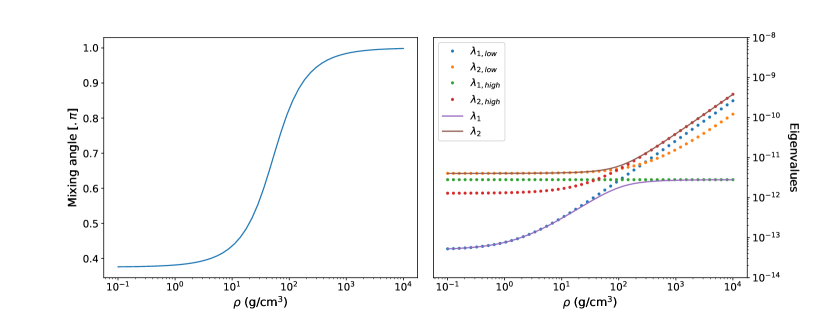
The behavior that is worth pointing out is that for high densities the first family eigenvalue equals the matter potential, and the mixing angle tends to $\pi$, which is a characteristic that can be found when expanding the analysis to 3 neutrino families in the next section.

In spite of the two neutrino families analysis having a well-defined and simplified description, we will work on a more realistic case, which considers the neutrinos three families. To simplify our analisys we will set $\delta_{CP}=0$ in what follows. For this specific case, the explicit form of the Hamiltonian in the flavor basis can be written as

$$H=U_{23}U_{13}U_{12}\left(\begin{array}[]{ccc}\frac{m^{2}_{1}}{2E_{\nu}}&0&0\\ 0&\frac{m^{2}_{2}}{2E_{\nu}}&0\\ 0&0&\frac{m^{2}_{3}}{2E_{\nu}}\end{array}\right)U_{12}^{\dagger}U_{13}^{\dagger}U_{23}^{\dagger}+\left(\begin{array}[]{ccc}V_{CC}&0&0\\ 0&0&0\\ 0&0&0\end{array}\right).$$

(25)

The Hamiltonian in Eq. (25) can be analyzed using the same approach as in Eq. (21), previously employed for the two-family regime. However, the key distinction in the three-family case lies in the presence of an additional eigenvalue, arising from the increased dimensionality of the system. The analysis will explore the behavior of the system in the low, intermediate, and high-density limits.

Low densities: $V_{CC}\sin(2\theta_{13})<\frac{\Delta m^{2}_{31}}{4E_{\nu}}$, $\frac{\Delta m^{2}_{21}}{4E_{\nu}}$

Since $V_{CC}$ only affects $H_{11}$, the mixing angle $\theta_{23}$ can be rotated out redefining $\nu_{\alpha}^{\prime}=U_{23}^{\dagger}\nu_{\alpha}$. If we also rotate out $\theta_{13}$, defining a $\nu_{\alpha}^{\prime\prime}=U_{13}^{\dagger}\nu_{\alpha}^{\prime}=U_{13}^{\dagger}U_{23}^{\dagger}\nu_{\alpha}$ we get:

$\displaystyle H^{{}^{\prime\prime}}=\frac{m_{1}^{2}+m_{2}^{2}}{4E_{\nu}}+\left(\begin{array}[]{ccc}-\delta_{21}c_{2\theta_{12}}&\delta_{21}s_{2\theta_{12}}&0\\ \delta_{21}s_{2\theta_{12}}&\delta_{21}c_{2\theta_{12}}&0\\ 0&0&\delta_{31}+\delta_{32}\end{array}\right)+V_{CC}\left(\begin{array}[]{ccc}c^{2}_{13}&0&s_{13}c_{13}\\ 0&0&0\\ s_{13}c_{13}&0&s^{2}_{13}\end{array}\right).$

(32)

where $\delta_{ji}=\Delta m^{2}_{ji}/4E_{\nu}$. For low densities we disregard the non-diagonal entry in the third term in right side of Eq. 32, decoupling our system into 2+1. It straightforward to obtain the third eigenvalue, related to the decoupled family:

$\displaystyle\lambda_{3}$

$\displaystyle=$

$\displaystyle\frac{m_{3}^{2}}{2E_{\nu}}+V_{CC}s^{2}_{13}.$

(33)

The remaining problem is solved by the diagonalization process of the non-diagonal subspace, which results in

$\displaystyle\lambda_{1,2}$

$\displaystyle=$

$\displaystyle\frac{m_{1}^{2}+m_{2}^{2}}{4E}+\frac{V_{CC}c^{2}_{13}}{2}\pm\sqrt{\left(\delta_{21}c_{2\theta_{12}}-\frac{V_{CC}c^{2}_{13}}{2}\right)^{2}+\left(\delta_{21}s_{2\theta_{12}}\right)^{2}}.$

(34)

The reduced 2-dimensional subsystem has an analytical solution for the mixing angle, as already shown in Eq. (23), which gives

$$\tan(2\tilde{\theta}_{12})=\frac{\frac{\Delta m^{2}}{4E_{\nu}}s_{2\theta_{12}}}{\frac{\Delta m^{2}}{4E_{\nu}}c_{2\theta_{12}}-\frac{V_{CC}}{2}c_{13}^{2}}.$$

(35)

This modification leads to the following change in the mixing matrix

$$\nu_{\alpha}^{\prime\prime}=\tilde{U}_{12}\nu_{i}~{}~{}~{}\rightarrow~{}~{}~{}U=U_{23}U_{13}\tilde{U}_{12}.$$

In Fig. 2 we present $\tilde{\theta}_{12}$ and eigenvalues as a function of density. The analytical expressions are reliable up to $\rho\sim 10^{3}$ g/cm³.

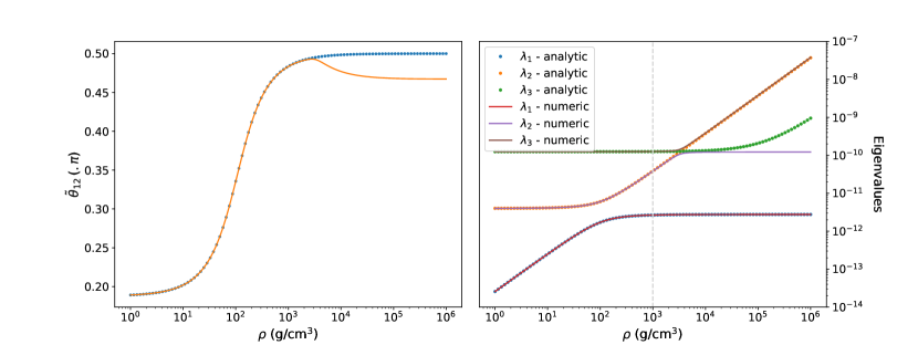
One interesting feature is that $\lambda_{1}$ provides a good approximation in the full range. The asymptotic value for large densities is

	$\displaystyle\lambda_{1}$	$\displaystyle=$	$\displaystyle\frac{m_{1}^{2}+m_{2}^{2}}{4E}+\frac{V_{CC}c^{2}_{13}}{2}-\frac{V_{CC}c^{2}_{13}}{2}\sqrt{1-4\delta_{21}c_{2\theta_{12}}\frac{1}{V_{CC}c^{2}_{13}}+\left(\frac{2}{V_{CC}c^{2}_{13}}\delta_{21}\right)^{2}}$
		$\displaystyle\sim$	$\displaystyle\frac{m_{1}^{2}}{2E}s^{2}_{12}+\frac{m_{2}^{2}}{2E}c^{2}_{12}.$

Since $\theta_{13}$ is small, this approximation should still be valid in the first resonance, $\tilde{\theta}_{12}=\pi/4$.

intermediate to high densities: $V_{CC}\sin(2\theta_{13})\gtrsim\frac{\Delta m^{2}_{31}}{4E_{\nu}}\gg\frac{\Delta m^{2}_{21}}{4E_{\nu}}$

If we take $\Delta m^{2}_{21}=0$, we have:

$$H=U_{23}U_{13}U_{12}\left(\begin{array}[]{ccc}\frac{m^{2}_{1}}{2E_{\nu}}&0&0\\ 0&\frac{m^{2}_{1}}{2E_{\nu}}&0\\ 0&0&\frac{m^{2}_{3}}{2E_{\nu}}\end{array}\right)U_{12}^{\dagger}U_{13}^{\dagger}U_{23}^{\dagger}+\left(\begin{array}[]{ccc}V_{CC}&0&0\\ 0&0&0\\ 0&0&0\end{array}\right).$$

Now, besides absorbing $U_{23}$ in $\nu^{\prime}$, we can perform the multiplication with $U_{12}$, arriving at:

$$H^{\prime}=U_{13}\left(\begin{array}[]{ccc}\frac{m^{2}_{1}}{2E_{\nu}}&0&0\\ 0&\frac{m^{2}_{1}}{2E_{\nu}}&0\\ 0&0&\frac{m^{2}_{3}}{2E_{\nu}}\end{array}\right)U_{13}^{\dagger}+\left(\begin{array}[]{ccc}V_{CC}&0&0\\ 0&0&0\\ 0&0&0\end{array}\right).$$

Now is the second family that gets decoupled, and we can use the expressions for the 2-families. In this case, the eigenvalues and mixing angles can be respectively written as

$$\lambda_{2,3}=\frac{m_{1}^{2}+m_{3}^{2}}{4E}+\frac{V_{CC}}{2}\pm\sqrt{\left(\frac{\Delta m_{31}^{2}}{4E_{\nu}}c_{2\theta_{13}}-\frac{V_{CC}}{2}\right)^{2}+\left(\frac{\Delta m_{31}^{2}}{4E_{\nu}}s_{2\theta_{13}}\right)^{2}},$$

(36)

$$\tan(2\tilde{\theta}_{13})=\frac{\frac{\Delta m_{31}^{2}}{4E_{\nu}}s_{2\theta_{13}}}{\frac{\Delta m_{31}^{2}}{4E_{\nu}}c_{2\theta_{13}}-\frac{V_{CC}}{2}}.$$

(37)

It is interesting to note that the asymptotic value of $\lambda_{3}$ for low energies agrees with Eq. (33) at first order in $\rho$.

In summary, we have so far the following approximations:

• •

  $\lambda_{1}$ (Eq. (34)) and $\lambda_{3}$ (Eq. (36)) valid for all ranges of $\rho$.

• •

  $\theta_{13}$ (Eq. (37)) also valid for all ranges of $\rho$.

• •

  $\lambda_{2}$ for low densities (around first resonance) given by Eq. (34) and a different expression for high densities (around second resonance), Eq. (36).

• •

  $\theta_{12}$ for low densities, given by Eq. (35).

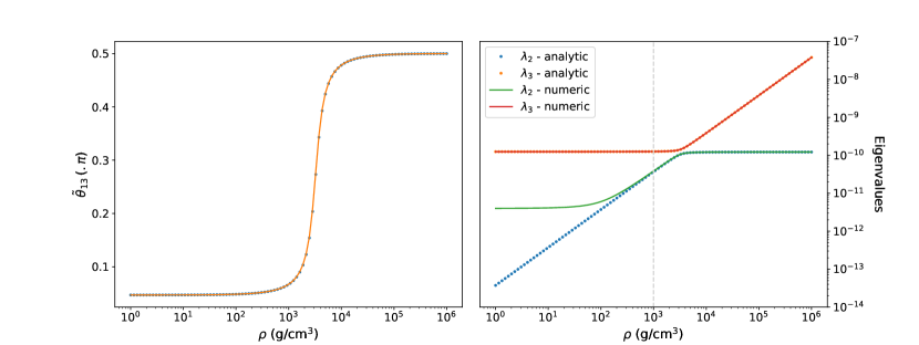
What is lacking is a expression for $\theta_{12}$ and $\theta_{23}$ for densities larger than the second resonance. Since we have reliable expressions for the other angles, it can be calculated as follows.

For very large densities $\tilde{\theta}_{13}\sim\pi/2$, and we can write

$$\cos\tilde{\theta}_{13}\sim\epsilon~{}~{}~{};~{}~{}~{}\sin\tilde{\theta}_{13}\sim 1-\frac{\epsilon^{2}}{2},$$

and the mixing matrix can be written in powers of $\epsilon$ as

$\displaystyle\tilde{U}=\left(\begin{array}[]{ccc}0&0&1\\ \lx@intercol\hfil\mathcal{O}\hfil\lx@intercol&\begin{array}[]{c}0\\ 0\end{array}\end{array}\right)+\epsilon\left(\begin{array}[]{ccc}c_{12}&s_{12}&0\\ \lx@intercol\hfil 0\hfil\lx@intercol&\begin{array}[]{c}s_{23}\\ c_{23}\end{array}\end{array}\right)+\frac{\epsilon^{2}}{2}\left(\begin{array}[]{ccc}0&0&-1\\ c_{12}s_{23}&s_{12}s_{23}&0\\ c_{12}c_{23}&s_{12}c_{23}&0\end{array}\right),$

(49)

where $\mathcal{O}$ can be written as a mixing matrix in 2 dimensions through a new angle $\alpha$:

$$\mathcal{O}=\left(\begin{array}[]{cc}-s_{12}c_{23}-c_{12}s_{23}&c_{12}c_{23}-s_{12}s_{23}\\ s_{12}s_{23}-c_{12}c_{23}&-c_{12}s_{23}-s_{12}c_{23}\end{array}\right)=\left(\begin{array}[]{cc}\cos\alpha&\sin\alpha\\ -\sin\alpha&\cos\alpha\end{array}\right).$$

Using Eq.(25) and the new parametrization in Eq.(49), the following relation

$$\tilde{U}\textrm{diag}(\tilde{\lambda}_{1},\tilde{\lambda}_{2},\tilde{\lambda}_{3})\tilde{U}^{\dagger}=U\textrm{diag}(\lambda_{1},\lambda_{2},\lambda_{3})U^{\dagger}+V_{CC}.$$

can be examined. To first order in $\epsilon$ and considering $\tilde{\lambda}_{3}\gg\tilde{\lambda}_{1,2}$, the left side becomes:

$$\frac{\tilde{\lambda}_{1}+\tilde{\lambda}_{2}}{2}+\left(\begin{array}[]{ccc}\frac{\Delta_{31}+\Delta_{32}}{2}&\epsilon\tilde{\lambda}_{3}s_{23}&\epsilon\tilde{\lambda}_{3}c_{23}\\ \begin{array}[]{c}\epsilon\tilde{\lambda}_{3}s_{23}\\ \epsilon\tilde{\lambda}_{3}c_{23}\end{array}&\lx@intercol\hfil h_{2\times 2}\hfil\lx@intercol\end{array}\right),$$

where

$$h_{2\times 2}=O\left(\begin{array}[]{cc}-\Delta_{21}/2&0\\ 0&+\Delta_{21}/2\end{array}\right)O^{\dagger}=\frac{\Delta_{21}}{2}\left(\begin{array}[]{cc}-\cos 2\alpha&\sin 2\alpha\\ \sin 2\alpha&\cos 2\alpha\end{array}\right),$$

and $\Delta_{ji}=(\tilde{\lambda}_{j}-\tilde{\lambda}_{i})/2$. Comparing with the left side of Eq. (25), we can finally write:

$$\tan\tilde{\theta}_{23}=(H_{mat})_{12}/(H_{mat})_{13}.$$

Explicitly, after some algebraic manipulation, we obtain the following expression

$$\tan\tilde{\theta}_{23}=\frac{(\Delta+\delta\cos 2\theta_{12})\sin 2\theta_{13}s_{23}+2\delta c_{13}\sin 2\theta_{12}c_{23}}{(\Delta+\delta\cos 2\theta_{12})\sin 2\theta_{13}c_{23}-2\delta c_{13}\sin 2\theta_{12}s_{23}}.$$

The relation between $\alpha$ and mixing angles $\theta_{12}$ and $\theta_{23}$ can be written realizing that:

$$\mathcal{O}=\left(\begin{array}[]{cc}-s_{12}c_{23}-c_{12}s_{23}&c_{12}c_{23}-s_{12}s_{23}\\ s_{12}s_{23}-c_{12}c_{23}&-c_{12}s_{23}-s_{12}c_{23}\end{array}\right)=\left(\begin{array}[]{cc}-s_{12}&c_{12}\\ -c_{12}&-s_{12}\end{array}\right)\left(\begin{array}[]{cc}c_{23}&s_{23}\\ -s_{23}&c_{23}\end{array}\right),$$

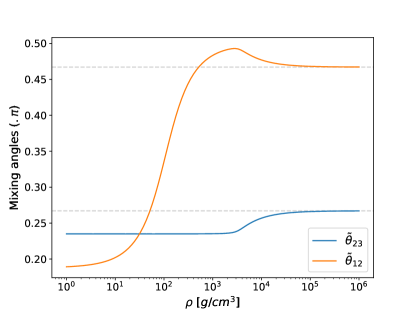
so $\alpha$ can be related to a rotation of $\theta_{23}$ followed by a rotation of $\theta_{12}+\pi/2$. Then

$$\tilde{\theta}_{12}=\alpha-\frac{\pi}{2}-\tilde{\theta}_{23},$$

so, after finding $\tilde{\theta}_{23}$ it is straightforward to find the value of $\tilde{\theta}_{12}$. In Fig. (4) we can see that the asymptotic value agrees with the numerical calculation.

References

- Fukuda et al. [1998] Y. Fukuda et al. (Super-Kamiokande), Evidence for oscillation of atmospheric neutrinos, Phys. Rev. Lett. 81, 1562 (1998), arXiv:hep-ex/9807003 .
- Ahmad et al. [2001] Q. R. Ahmad et al. (SNO), Measurement of the rate of interactions produced by 8B solar neutrinos at the Sudbury Neutrino Observatory, Phys. Rev. Lett. 87, 071301 (2001), arXiv:nucl-ex/0106015 .
- Cai et al. [2017] Y. Cai, J. Herrero-García, M. A. Schmidt, A. Vicente, and R. R. Volkas, From the trees to the forest: a review of radiative neutrino mass models, Front. in Phys. 5, 63 (2017), arXiv:1706.08524 [hep-ph] .
- Dell’Oro et al. [2016] S. Dell’Oro, S. Marcocci, M. Viel, and F. Vissani, Neutrinoless double beta decay: 2015 review, Adv. High Energy Phys. 2016, 2162659 (2016), arXiv:1601.07512 [hep-ph] .
- Dolinski et al. [2019] M. J. Dolinski, A. W. P. Poon, and W. Rodejohann, Neutrinoless Double-Beta Decay: Status and Prospects, Ann. Rev. Nucl. Part. Sci. 69, 219 (2019), arXiv:1902.04097 [nucl-ex] .
- Giunti and Kim [2007] C. Giunti and C. W. Kim, Fundamentals of Neutrino Physics and Astrophysics (2007).
- Navas et al. [2024] S. Navas et al. (Particle Data Group), Review of particle physics, Phys. Rev. D 110, 030001 (2024).
- de Gouvêa et al. [2022] A. de Gouvêa, G. Jusino Sánchez, and K. J. Kelly, Very light sterile neutrinos at NOvA and T2K, Phys. Rev. D 106, 055025 (2022), arXiv:2204.09130 [hep-ph] .
- Suekane and de Castro Bezerra [2016] F. Suekane and T. J. de Castro Bezerra, Double chooz and a history of reactor 13 experiments, Nuclear Physics B 908, 74 (2016).
- Nath and Francis [2021] A. Nath and N. K. Francis, Detection techniques and investigation of different neutrino experiments, International Journal of Modern Physics A 36, 2130008 (2021).
- Adamson et al. [2020] P. Adamson et al. (MINOS+), Precision Constraints for Three-Flavor Neutrino Oscillations from the Full MINOS+ and MINOS Dataset, Phys. Rev. Lett. 125, 131802 (2020), arXiv:2006.15208 [hep-ex] .
- Abe et al. [2023] K. Abe et al. (T2K), Updated T2K measurements of muon neutrino and antineutrino disappearance using 3.6×10²¹ protons on target, Phys. Rev. D 108, 072011 (2023), arXiv:2305.09916 [hep-ex] .
- Kajita [2010] T. Kajita, Atmospheric neutrinos and discovery of neutrino oscillations, Proceedings of the Japan Academy, Series B 86, 303 (2010).
- Abbasi et al. [2023] R. Abbasi et al. ((IceCube Collaboration)*, IceCube), Measurement of atmospheric neutrino mixing with improved IceCube DeepCore calibration and data processing, Phys. Rev. D 108, 012014 (2023), arXiv:2304.12236 [hep-ex] .
- Abe et al. [2018] K. Abe et al. (Super-Kamiokande), Atmospheric neutrino oscillation analysis with external constraints in Super-Kamiokande I-IV, Phys. Rev. D 97, 072001 (2018), arXiv:1710.09126 [hep-ex] .
- Abe et al. [2024] K. Abe et al. (T2K, Super-Kamiokande), First joint oscillation analysis of Super-Kamiokande atmospheric and T2K accelerator neutrino data, (2024), arXiv:2405.12488 [hep-ex] .
- Li et al. [2018] Z. Li et al. (Super-Kamiokande), Measurement of the tau neutrino cross section in atmospheric neutrino oscillations with Super-Kamiokande, Phys. Rev. D 98, 052006 (2018), arXiv:1711.09436 [hep-ex] .
- Gando et al. [2011] A. Gando et al. (KamLAND), Constraints on from A Three-Flavor Oscillation Analysis of Reactor Antineutrinos at KamLAND, Phys. Rev. D 83, 052002 (2011), arXiv:1009.4771 [hep-ex] .
- Wolfenstein [1978] L. Wolfenstein, Neutrino Oscillations in Matter, Phys. Rev. D 17, 2369 (1978).
- Mikheyev and Smirnov [1985] S. P. Mikheyev and A. Y. Smirnov, Resonance Amplification of Oscillations in Matter and Spectroscopy of Solar Neutrinos, Sov. J. Nucl. Phys. 42, 913 (1985).