Analytical Solution for the Size of the Minimum Dominating Set
in Complex Networks
Abstract
Domination is the fastest-growing field within graph theory with a profound diversity and impact in real-world applications, such as the recent breakthrough approach that identifies optimized subsets of proteins enriched with cancer-related genes. Despite its conceptual simplicity, domination is a classical NP-complete decision problem which makes analytical solutions elusive and poses difficulties to design optimization algorithms for finding a dominating set of minimum cardinality in a large network. Here we derive for the first time an approximate analytical solution for the density of the minimum dominating set (MDS) by using a combination of cavity method and Ultra-Discretization (UD) procedure. The derived equation allows us to compute the size of MDS by only using as an input the information of the degree distribution of a given network.
pacs:
I Introduction
The research on complex networks in diverse fields newman ; caldarelli , based on applied graph theory combined with computational and statistical physics methods, has experienced a spectacular growth in recent years and has led to the discovery of ubiquitous patterns called scale-free networks barabasi , unexpected dynamic behavior vespignani , robustness and vulnerability features havlin1 ; reka ; motter , and applications in natural and social complex systems newman ; caldarelli . On the other hand, domination is an important problem in graph theory which has rich variants, such as independence, covering and matching teresa . The mathematical and computational studies on domination have led to abundant applications in disparate fields such as mobile computing and computer communication networks sto , design of large parallel and distributed systems swapped , analysis of large social networks social1 ; social2 ; social3 , computational biology and biomedical analysis vazquez and discrete algorithms research teresa .
More recently, the Minimum Dominating Set (MDS) has drawn the attention researchers to controllability in complex networks nacher1 ; nacher2 ; nacher3 , to investigate observability in power-grid power and to identify an optimized subset of proteins enriched with essential, cancer-related and virus-targeted genes in protein networks wuchty . The size of MDS was also investigated by extensively analysing several types of artificial scale-free networks using a greedy algorithm in molnar . The problem to design complex networks that are structurally robust has also recently been investigated using the MDS approach nacher4 ; molnar2 .
Despite its conceptual simplicity, the MDS is a classical NP-complete decision problem in computational complexity theory johnson . Therefore, it is believed that there is no a theoretically efficient (i.e., polynomial time) algorithm that finds an exact smallest dominating set for a given graph. It is worth noticing that although it is an NP-hard problem, recent results have shown that we can use Integer Linear Programming (ILP) to find optimal solution nacher1 ; wuchty ; nacher4 . Moreover, for specific types of graph such a tree (i.e., no loops) and even partial--tree, it can be solved using Dynamic Programing (DP) in polynomial time akutsu .
Especially, the density (or fraction) of MDS, defined as the size of MDS versus the total number of nodes in a network, is important to estimate the cost-efficient network deployment of controllers. It is less expensive to have ten power plants operating as controllers in a large network of 1,000 sites than one hundred. Similarly, acting on two protein targets via drug interactions is always better than acting on ten protein targets to minimize adverse side effects. Although we can use an ILP method for obtaining an MDS and the density of MDS, we do not have an analytic solution for the density of MDS. Note that even though optimal solution for MDS can be found using ILP method, this kind of technique is very generic and operates as a black box so that its systematic application does not provide us any knowledge about the details of the particular problem under study. Moreover, from a physical point of view, analytic solutions always enable us to have a deeper understanding of the problem by examining dependences with other variables. Here, we derive for the first time an analytical solution for an MDS by using cavity method.
Cavity method is a well-known methodology developed by physicists working on statistical mechanics (e.g. spin glasses spin ). However, this technique has also been extended and applied to non-physical systems, including network theory in which nodes can be abstracted to some extent. For example, applications include the analysis of random combinatorial problems such as weighted matching mezard1 , the vertex cover hart and the travelling salesman problem mezard2 . Moreover, recently cavity method was used to determine the number of matchings in random graphs mezard_last , the maximal independent sets dalla , the random set packing indian and the minimum weight Steiner tree steiner and controllability using maximum matching liu , extending the work done in mezard_last for undirected networks to directed networks.111Note added: After finishing our paper, we became aware of a recent paper done independently by Zhao et al.Zhao , in which the statistical properties of the MDS were studied. Although the starting point of the cavity analysis is similar, in their results they estimate ths size of MDS by population dynamics simulations. In contrast, as shown later, we derive analytical solution for the size of the MDS. It is also well-known that cavity method computed at zero temperature limit has been applied to networks and used in many works, which have led to derive elegant analytical formulas new1 ; new2 ; new3 .
On the other hand, the Ultra Discretization (UD) procedure has been developed mainly in the field of soliton theory and cellular automaton (CA) theory UD1 ; UD2 ; UD3 ; UD4 ; UDours . Although the common discretization process discretizes independent variables, the UD procedure can discretize dependent variables. As a result, both independent and dependent variables become discrete variables. In other words, UD transforms discretized equations into their corresponding UD equations. In soliton theory, we can obtain the cellular automaton from the corresponding discretized soliton theory after UD procedure. In UD4 , it is shown that the corresponding integrable CA is obtained from Korteweg–de Vries (KdV) soliton equation via Lotka-Volterra equation, using UD procedure. The key point of UD is that the UD procedure can be applied only in the case that the original discretized equation does not have any minus operators.
By combining the cavity method and UD procedure, we solved for the first time the density of MDS problem analytically for any complex network. By cavity method and UD, we derived a combinatorial expression that allows us to identify the density of MDS by only using the degree distribution of the network, which is our main result. We then compare the results of the derived expression for density of MDS with the ILP solutions for regular, random and scale-free networks showing a fair agreement. Moreover, a simple formula is derived for random networks at the large degree limit.
II Theoretical results
II.1 The Hamiltonian of a dominating set
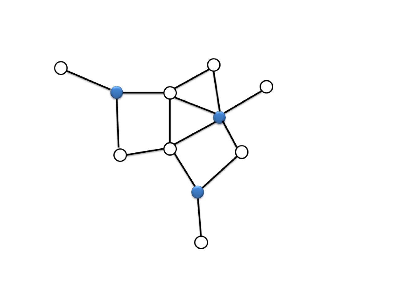
A graph is a set of nodes and edges . A Dominant Set (DS) is defined to be a subset of , where each node belongs to or adjacent to an element of . For each node , we define a binary function to be if , otherwise . We call the node occupied (resp. empty) if is (resp. ). The set of the adjacent nodes to node is denoted by . We can then see that the constraint to define a DS is as follows:
| (1) |
For each node , we define a binary function to be if and only if , otherwise 0. A set is an Minimum Dominating Set (MDS) if the size is smallest among all dominating sets (see Fig. 1).
Let us consider the following Hamiltonian function:
| (2) |
where . Then the partition function is given by
| (3) |
where the summation is taken over all configurations of and is the inverse temperature.
II.2 Cavity method analysis
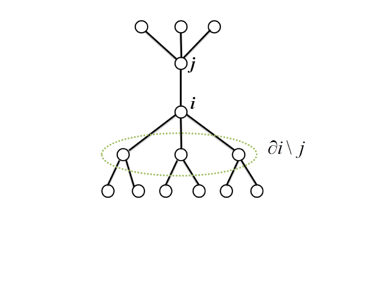
In what follows, we apply the cavity method to derive the analytic formula for the density of MDS in complex networks. Note that the cavity approach has been used in a similar way to solve the maximal independent set problem dalla . First, we assume the graph has tree structure and let be the set of except for node (see Fig. 2). Note also that the minimum degree of the graph should be two, otherwise some of do not exist. Then, we can write . Next, let be the probability that the node and take value and , respectively, and constraints and are not included:
| (4) |
where the first summation is taken over all configurations of . The product for the constraint is taken over all nodes of except for , (i.e. and ) and is the normalization constant given by
| (5) | |||||
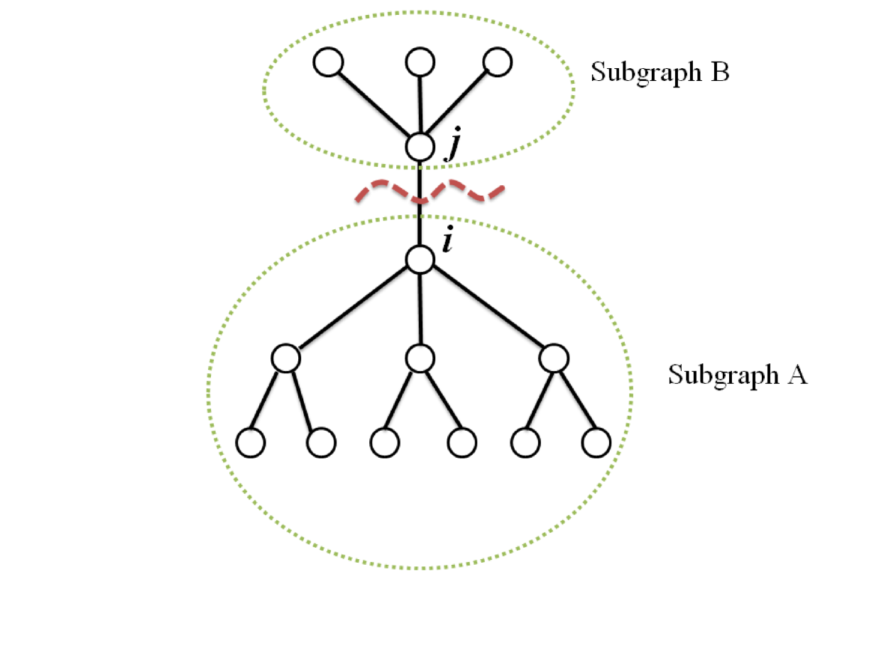
Eq. (4) can be written in a different way, which will be easier to compute. As shown in Fig. 3, we divide a graph into two subgraphs ( and ) by cutting the edge (, ) between node and . Let be the set of all the nodes which belongs to the subgraph including , and be the set of all the nodes which belongs to the subgraph including . Then, Eq. (4) can be transformed into
| (6) |
where the first summation is taken over all configurations of . The product for the constraint is taken over all nodes of except (i.e. and ) and is a normalization constant given by
| (7) | |||||
where the last summation is taken over all configurations of .
Then the following exact recursive equation can be derived:
| (8) |
This equation can be iteratively solved with its corresponding normalization constant.
Let be the summation of , where the number of occupied neighbors is :
| (9) |
Then, let be the probability that the node is occupied in the cavity graph. Let be the probability that the node and all the neighbors are empty. Let be the probability that the node is empty and at least one of the neighbors are occupied. Then, we can write:
| (10) | |||||
| (11) | |||||
| (12) |
where is the degree of node . Here we note that , because of probability normalization.
The above definitions lead to the following iterative equations:
| (13) | |||||
| (14) | |||||
| (15) |
where is the normalization constant given by
| (16) |
II.3 Ultra-Discretization (UD) procedure
We note that until now we are considering the problem of an DS, which is treated as finite temperature problem ( is finite) in the context of statistical mechanics. To address the minimum dominating set (MDS) problem, we have to consider the zero-temperature limit () which gives the ground energy state of the Hamiltonian shown in Eq. (2). To solve the equations associated to the zero-temperature limit, we can use an Ultra-Discretization (UD) procedure UD4 .
| Equation | independent variable | dependent variable |
|---|---|---|
| () Continuous equation for | : real value | : real value |
| () Discretized equation for | : integer | : real value |
| () Ultra- Discretized (UD) equation for | : integer | : integer |
Discretization is a well-known method to discretize independent variable in continuous theory such as differential equation (see Table 1 from () to ()). UD can go further and aims to discretize the dependent variable in the discretized equation (from () to ()). As a result, in the transformed UD equation (), both independent and dependent variables are discretized (i.e. both are integer variables). The key formula of UD, which transforms the equation type from () to () is
| (17) |
When the discretized equation () has no subtraction operator, we can transform it into the corresponding UD equation () by replacing and and taking limit . Here, and belong to discretized equation () and and belong to UD equation (). The operator in the original discretized equation () is transformed in the UD equation () as follows:
| (18) | |||
| (19) | |||
| (20) |
Here we remark that in order to obtain the UD equation (), it is necessary to be able to remove any minus operator in the original discretized equation ().
In order to ultra-discretize the previous Eqs. (13), (14) and (15), we make them consist of only plus, multiplication and division operators, avoiding minus operators. By simple computation, we have
| (21) |
and
| (22) |
where is the number of elements of , and .
By inserting Eqs. (21) and (22) into Eqs. (13), (14) and (15), we have
| (23) | |||||
| (24) | |||||
| (25) |
Here we remark that the above derived equations consist only of three operators (plus, multiplication and division), which is suitable for the ultra-discretization.
Here, we then replace the following three variables as follows:
| (26) | |||||
| (27) | |||||
| (28) |
where , and are variables in UD system.
After inserting (26), (27), (28) into (23), (24), (25) and taking zero-temperature limit , Eqs. (23), (24) and (25) are transformed into
| (29) | |||||
| (30) | |||||
Eq. (23), (24), (25) (or Eq. (29), (30), (LABEL:eqn:UD_equation_3)) are very difficult to solve, because every edge direction has three variables and three associated equations. Therefore, in order to avoid this high complexity, we use a coarse-grained method.
Let be the degree distribution of the network which gives the probability to find nodes with degree and be the average degree of the network. The excess degree distribution is given by , that is the probability to find that a neighbor node has degree k.
Let us assume that the network is enough large. Each and values are assigned to the edge direction from to . The opposite edge direction gets the values from and . is not independent variable because of the normalization. Let be the probability density function of , .
Then we have the coarse-grained equation (cavity mean field equation) for (23) and (25) as follows:
| (32) | |||||
We transform the probability density function by variables transformation (26) and (28) as follows:
| (33) |
Then, we have
| (34) | |||||
Taking UD limit (zero temperature) , we have the ultra-discretization version of cavity equation:
Next, we will solve this equation. Eqs. (29), (30), (LABEL:eqn:UD_equation_3) imply that and takes integer values, since and at the boundary of network takes integer values. Furthermore, considering the probability conservation, Eqs. (26), (28) imply that and takes value 0 or negative integer. By considering Eq. (29), firstly, we can see that takes value only or . Secondly, if is , then for each , one of or takes value . In this case (), from Eq. (LABEL:eqn:UD_equation_3), takes value or . Therefore, we can set the distribution as follows:
| (36) |
where .
Inserting (36) into the cavity equation (LABEL:eqn:_cavity_equation_UD), we have
| (37) | |||||
| (38) | |||||
| (39) |
Once the degree distribution is given, we can determine , , .
Here, we need the average energy of the Hamiltonian (2), which can be identified as the average number of all DS configurations. After taking zero temperature limit , we will obtain the analytical formula for the density of MDS.
The average energy can be computed by , where the partition function is shown in Supplementary Information. A generic expression for density is given by
| (40) | |||||
This equation, however, cannot be ultra-discretized because of the minus operator, and without being ultra-discretized, analytical solution cannot be obtained. Therefore, we avoid minus operator by inserting Eqs. (21) and (22), which leads to the following result:
| (41) |
After taking zero temperature limit , we obtain
| (42) |
By inserting (36) into this equation, we finally obtain
| (43) | |||||
More simply, we transform the previous equation into
Eq. (LABEL:eqn:_analytic_formula2) is our main result. Using this equation, we can analytically compute the density of MDS from any degree distribution . More concretely, we can summarize the procedure as follows. Once the degree density function is given, we can easily compute the excess degree density function . Then, by solving (37), (38) and (39), we obtain , , . Finally, inserting the value , , into the above equation (LABEL:eqn:_analytic_formula2), we obtain the density of MDS.
We note that when we consider random network with average degree as a special case, we can derive the simple expression by using large average degree limit approximation () (See supplementary Information).
III Computational results
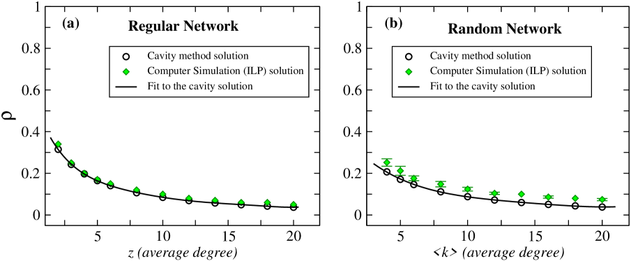
Here we performed computer simulations to examine the theoretical results (LABEL:eqn:_analytic_formula2) obtained using cavity method. First, we consider regular and random networks constructed with a variety of average degree values (see Fig. 4 (a) and (b)). The results show that cavity method predictions are in excellent agreement with ILP solutions.
Next, we examine the case of scale-free networks. We first generated samples of synthetic scale-free networks
with a variety of scaling exponent and average degree using the Havel-Hakimi algorithm with random edge swaps (HMC). All
samples were generated with a size of nodes. We investigated two different cases. We constructed a set of scale-free
network samples with natural cut-off and
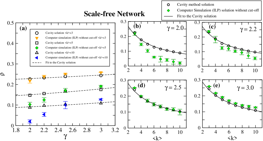
another set with structural cut-off . The minimum degree is in both cases. Fig. 5
shows the results for natural cut-off (i.e. no structural cut-off is considered). The dependence of the MDS density as a function of
the average degree shows a good agreement with the cavity method analytical predictions (LABEL:eqn:_analytic_formula2), in particular
when increases (see Figs. 5 (c)-(e)). By increasing the average degree, the MDS density
decreases. For small values of , the predictions of the cavity method deviates from the ILP solutions when average degree
increases (see Fig. 5(b)). The reason is because in this case, the network tends to have hubs with
very high degree. While these hubs are still visible to ILP method, they are not observed by the cavity method. It is well-known
that cavity method addresses better homogeneous networks than extremely inhomogeneous networks. On the other hand, by examining
the function of MDS density versus , we clearly observe the
influence of the average degree (see Fig. 5(a)). Moreover, in absence of
structural cut-off, for high average degree networks, the MDS density for ILP decreases faster than the solution for cavity method when decreases.
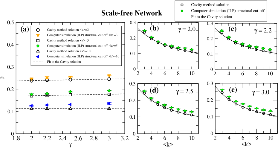
We have also considered the case of structural cut-off when constructing finite artificial scale-free networks
to address the finite-size effect and eliminate degree correlations.
The computer simulations on scale-free networks with structural cut-off shows a different picture
(see Fig. 6(a)-(e)). The MDS density does not significantly
changes when decreases and remains constant along all the range of values
(see Fig. 6(a)). Moreover, when structural cut-off is considered, the agreement
between cavity method and ILP results becomes more evident for any value of and average degree (see Fig. 6 (b)-(e)). The reason is because the network tends to be more
homogeneous when some hubs with extremely high-degree are knocked out by the structural cut-off.
IV Conclusion
Domination is not only one of the most active research areas in graph theory but also has found abundant real-world applications in many different fields, from engineering to social and natural sciences. With the recent years expansion of networks as data representation framework, domination techniques may provide a rich set of tools to face current network problems in society and nature.
In this work, by using the cavity method and the ultra-discretization procedure, we solved for the first time the MDS problem analytically and derived a combinatorial equation whose computation is easier than that of ILP. By only using the degree distribution of a network as an input information, we can compute the density of an MDS and investigate any dependence with respect to other network variables without using assistance of any complex optimization methods such as ILP or DP.
The present analysis may allow a variety of rich extensions such as computing the corresponding analytical expression for MDS density in directed and bipartite networks.
V Acknowledgements
We thank Prof. Tatsuya Akutsu for insighful comments. J.C.N. was partially supported by MEXT, Japan (Grant-in-Aid No. 25330351), and T.O. was partially supported by JSPS Grants-in-Aid for Scientific Research (Grant Number 15K01200) and Otsuma Grant-in Aid for Individual Exploratory Research (Grant Number S2609).
References
- (1) M.E.J. Newman, Networks: An Introduction. (Oxford University Press, New York, 2010)
- (2) G. Caldarelli, Scale-Free Networks: Complex Webs in Nature and Technology (Oxford Univ. Press, Oxford, 2007).
- (3) A.-L. Barabási, R. Albert, Science 286, 509 (1999).
- (4) R. Pastor-Satorras, A. Vespignani, Phys. Rev. Lett. 86, 3200 (2001).
- (5) R. Cohen, K. Erez, D. ben-Avraham and S. Havlin, Phys. Rev. Lett. 85, 4626 (2000).
- (6) R. Albert, H. Jeong, A.-L. Barabasi, Nature 406, 378 (2000).
- (7) A. E. Motter, Phys. Rev. Lett. 93, 098701 (2004).
- (8) T.W. Haynes, S.T. Hedetniemi and P.J. Slater, Fundamentals of Domination in Graphs (Pure Applied Mathematics, Chapman and Hall/CRC, New York, 1998).
- (9) I. Stojmenovic, M. Seddigh and J. Zunic, IEEE Trans. Parallel Distributed Systems 13, 14 (2002).
- (10) W. Chena, Z. Lub and W. Wub, Information Sciences 269, 286 (2014).
- (11) L. Kelleher and M. Cozzens, Graphs. Math. Soc. Sciences 16, 267 (1988).
- (12) F. Wang, et al. , Theo. Comp. Sci. 412, 265 (2011).
- (13) S. Eubank, V.S. Anil Kumar, M.V. Marathe, A. Srinivasan and N. Wang, in SODA ’04 Proceedings of the fifteenth annual ACM-SIAM symposium on Discrete algorithms pp. 718-727 (2004).
- (14) A. Vazquez, BMC Systems Biology 3, 81 (2009).
- (15) J.C. Nacher and T. Akutsu, New J. Phys. 14, 073005 (2012).
- (16) J.C. Nacher and T. Akutsu, Journal of Physics: Conf. Ser. 410, 012104 (2013).
- (17) J.C. Nacher and T. Akutsu, Scientific Reports 3, 1647 (2013).
- (18) Y. Yang, J. Wang and A.E. Motter, Phys. Rev. Lett. 109, 258701 (2012).
- (19) S. Wuchty, Proc. Natl. Acad. Sci. USA 111, 7156 (2014).
- (20) F. Molnár, S. Sreenivasan, B.K. Szymanski and G. Korniss, Scientific Reports 3, 1736 (2013).
- (21) J.C. Nacher and T. Akutsu, Phys. Rev. E 91, 012826 (2015).
- (22) F. Molnár, N. Derzsy, B.K. Szymanski and G. Korniss, Scientific Reports 5, 8321 (2015).
- (23) M. Garey, and D.S. Johnson, Computers and Intractability: A Guide to the Theory of NP-Completeness, (W. H. Freeman, 1979).
- (24) C. Cooper and M. Zito, Discrete Applied Mathematics 157, 2010 (2009).
- (25) M. Mezard, G. Parisi G and M.A. Virasoro, Spin-Glass Theory and Beyond (Lecture notes in Physics vol. 9) (World Scientific, Singapore, 1987)
- (26) M. Mezard and G. Parisi, J. Phys. Lett. 46 L771, (1985).
- (27) M. Weigt and A.K. Hartmann, Phys. Rev. Lett. 84 6118 (2000).
- (28) M. Mezard and G. Parisi, J. Physique 47 1285, (1986).
- (29) L. Zdeborova and M. Mezard, J. Stat. Mech. P05003 (2006).
- (30) L. Dall’Asta, P. Pin, and A. Ramezanpour, Phys. Rev. E 80, 061136 (2009).
- (31) C. Lucibello and F. Ricci-Tersenghi, Int. J. Statistical Mechanics vol. 2014, Article ID 136829, (2014)
- (32) M. Bayati, C. Borgs, A. Braunstein, J. Chayes, A. Ramezanpour, and R. Zecchina, Phys. Rev. Lett. 101, 037208 (2008).
- (33) Y.-Y. Liu, J.-J. Slotine, A.-L. Barabási, Nature 473, 167 (2011).
- (34) M. Mezard, G. Parisi, Journal of Statistical Physics 111, 1 (2003)
- (35) M. Mezard, F. Ricci-Tersenghi, R. Zecchina, Journal of Statistical Physics, 111, 505 (2003)
- (36) O. Rivoire, G. Biroli, O.C. Martin, M. Mezard, Eur. Phys. J. B, 37, 55 (2004)
- (37) D. Takahashi and J. Satsuma, J. Phys. Soc. Jpn. 59, 3514 (1990).
- (38) D. Takahashi, T. Tokihiro, B.Grammaticos, Y. Ohta, A Ramani, J. Phys. A 30 7953 (1997).
- (39) T. Tokihiro, D. Takahashi, J. Matsukidaira, J. Phys. A 33 607 (2000).
- (40) T. Tokihiro, D. Takahashi, J. Matsukidaira and J. Satsuma, Phys. Rev. Lett. 76 3247 (1996).
- (41) T. Ochiai, J.C. Nacher, Journal of Mathematical Physics 46 063507 (2005).
- (42) M. Bayati, C. Nair, http://arxiv.org/abs/cond-mat/0607290
- (43) J.H. Zhao, Y. Habibulla, H.J. Zhou Journal of Statistical Physics159 1154 (2015).