numbers=left, numberstyle=
Analyzing Smart Contracts: From EVM to a sound Control-Flow Graph
Abstract
The EVM language is a simple stack-based language with words of 256 bits, with one significant difference between the EVM and other virtual machine languages (like Java Bytecode or CLI for .Net programs): the use of the stack for saving the jump addresses instead of having it explicit in the code of the jumping instructions. Static analyzers need the complete control flow graph (CFG) of the EVM program in order to be able to represent all its execution paths. This report addresses the problem of obtaining a precise and complete stack-sensitive CFG by means of a static analysis, cloning the blocks that might be executed using different states of the execution stack. The soundness of the analysis presented is proved.
1 EVM Language
The EVM language is a simple stack-based language with words of 256 bits with a local volatile memory that behaves as a simple word-addressed array of bytes, and a persistent storage that is part of the blockchain state. A more detailed description of the language and the complete set of operation codes can be found in [6]. In this section, we focus only on the relevant characteristics of the EVM that are needed for describing our work. We will consider EVM programs that satisfy two constraints: (1) jump addresses are constants,i.e. they are introduced by a PUSH operation, they do not depend on input values and they are not stored in memory nor storage, and (2) the size of the stack when executing a jump instruction can be bounded by a constant. These two cases are mostly produced by the use of recursion and higher-order programming in the high-level language that compiles to EVM, as e.g. Solidity.
|
1contract EthereumPot {
2 address[] public addresses;
3 address public winnerAddress;
4 uint[] public slots;
5 function __callback (bytes32 _queryId, string _result, bytes _proof){
6 if (msg.sender != oraclize_cbAddress()) throw;
7 random_number = uint(sha3(_result))
8 winnerAddress = findWinner(random_number);
9 amountWon = this.balance * 98 / 100 ;
10 winnerAnnounced(winnerAddress, amountWon);
11 if (winnerAddress.send(amountWon)) {
12 if (owner.send(this.balance)) {
13 openPot();
14 }
15 }
16 }
17
18 function findWinner (uint random) constant returns (address winner) {
19 for (uint i = 0; i < slots.length; i++) {
20 if (random <= slots[i]) {
21 return addresses[i];
22 }
23 }
24 }
25 // Other functions
26}
|
|
⋯
64B: JUMPDEST
64C: PUSH1 0x00
64E: DUP1
64F: PUSH1 0x00
651: SWAP1
652: POP
653: JUMPDEST
654: PUSH1 0x03
656: DUP1
657: SLOAD
658: SWAP1
659: POP
65A: DUP2
65B: LT
65C: ISZERO
65D: PUSH2 0x06D0
660: JUMPI
661: PUSH1 0x03
663: DUP2
664: DUP2
665: SLOAD
666: DUP2
⋯
941: JUMPDEST
942: MOD
943: ADD
944: PUSH1 0x0A
946: DUP2
947: SWAP1
948: SSTORE
949: POP
94A: PUSH2 0x0954
94D: PUSH1 0x0A
94F: SLOAD
950: PUSH2 0x064B
953: JUMP
⋯
|
Example 1
In order to describe our techniques, we use as running example a simplified version (without calls to the external service Oraclize and the authenticity proof verifier) of the contract [1] that implements a lottery system. During a game, players call a method joinPot to buy lottery tickets; each player’s address is appended to an array addresses of current players, and the number of tickets is appended to an array slots, both having variable length. After some time has elapsed, anyone can call rewardWinner which calls the Oraclize service to obtain a random number for the winning ticket. If all goes according to plan, the Oraclize service then responds by calling the __callback method with this random number and the authenticity proof as arguments. A new instance of the game is then started, and the winner is allowed to withdraw her balance using a withdraw method. Figure 2 shows an excerpt of the Solidity code (including the public function findWinner) and a fragment of the EVM code produced by the compiler. The Solidity source code is shown for readability, as our analysis works directly on the EVM code.
|
1contract EthereumPot {
2 address[] public addresses;
3 address public winnerAddress;
4 uint[] public slots;
5 function __callback (bytes32 _queryId, string _result, bytes _proof){
6 if (msg.sender != oraclize_cbAddress()) throw;
7 random_number = uint(sha3(_result))
8 winnerAddress = findWinner(random_number);
9 amountWon = this.balance * 98 / 100 ;
10 winnerAnnounced(winnerAddress, amountWon);
11 if (winnerAddress.send(amountWon)) {
12 if (owner.send(this.balance)) {
13 openPot();
14 }
15 }
16 }
17
18 function findWinner (uint random) constant returns (address winner) {
19 for (uint i = 0; i < slots.length; i++) {
20 if (random <= slots[i]) {
21 return addresses[i];
22 }
23 }
24 }
25 // Other functions
26}
|
|
⋯
64B: JUMPDEST
64C: PUSH1 0x00
64E: DUP1
64F: PUSH1 0x00
651: SWAP1
652: POP
653: JUMPDEST
654: PUSH1 0x03
656: DUP1
657: SLOAD
658: SWAP1
659: POP
65A: DUP2
65B: LT
65C: ISZERO
65D: PUSH2 0x06D0
660: JUMPI
661: PUSH1 0x03
663: DUP2
664: DUP2
665: SLOAD
666: DUP2
⋯
941: JUMPDEST
942: MOD
943: ADD
944: PUSH1 0x0A
946: DUP2
947: SWAP1
948: SSTORE
949: POP
94A: PUSH2 0x0954
94D: PUSH1 0x0A
94F: SLOAD
950: PUSH2 0x064B
953: JUMP
⋯
|
To the right of Figure 2 we show a fragment of the EVM code of method findWinner. It can be seen that the EVM has instructions for operating with the stack contents, like DUPx or SWAPx; for comparisons, like LT, GT; for accessing the storage (memory) of the contract, like SSTORE, SLOAD (MLOAD, MSTORE); to add/remove elements to/from the stack, like PUSHx/ POP; and many others (we again refer to [6] for details). Some instructions increment the program counter in several units (e.g., PUSHx Y adds a word with the constant Y of x bytes to the stack and increments the program counter by ). In what follows, we use to refer to the number of units that instruction increments the value of the program counter. For instance , or .
One significant difference between the EVM and other virtual machine languages (like Java Bytecode or CLI for .Net programs) is the use of the stack for saving the jump addresses instead of having it explicit in the code of the jumping instructions. In EVM, instructions JUMP and JUMPI will jump, unconditionally and conditionally respectively, to the program counter stored in the top of the execution stack. This feature of the EVM requires, in order to obtain the control flow graph of the program, to keep track of the information stored in the stack. Let us illustrate it with an example.
Example 2
In the EVM code to the right of Figure 2 we can see two jump instructions at program points 953 and 660, respectively, and the jump address (64B and 6D0) is stored in the instruction immediately before them: 950 or 65D. It then jumps to this destination by using the instruction JUMPDEST (program points 941, 64B, 653).
We start our analysis by defining the set , which contains all possible jump destinations in an EVM program :
We use for referring to the instruction at program counter in the EVM program . In what follows, we omit from definitions when it is clear from the context, e.g., we use to refer to .
Example 3
Given the EVM code that corresponds to function findWinner, we get the following set:
The first step in the computation of the CFG is to define the notion of block. In general [2], given a program , a block is a maximal sequence of straight-line consecutive code in the program with the properties that the flow of control can only enter the block through the first instruction in the block, and can only leave the block at the last instruction. Let us define the concept of block in an EVM program:
Definition 1 (blocks)
Given an EVM program , we define
where
Example 4
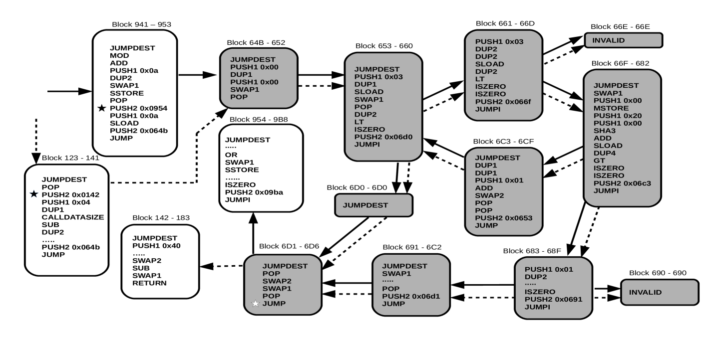
Figure 3 shows the blocks (nodes) obtained for findWinner and their corresponding jump invocations. Solid and dashed edges represent the two possible execution paths depending on the entry block: solid edges represent the path that starts from block 941 and dashed edges the path that starts from 123. Note that most of the blocks start with a JUMPDEST instruction (123, 941, 64B, 653, 66F, 954, 6C3, 691, 142, 6D1, 6D0). The rest of the blocks start with instructions that come right after a JUMPI instruction (661, 683). Analogously, most blocks end in a JUMP (941, 6C3, 123, 691, 6D1), JUMPI (653, 661, 66F, 683) or RETURN (142) instruction or in the instruction that precedes JUMPDEST (64B).
Observing the blocks in Figure 3, we can see that most JUMP instructions use the address introduced in the PUSH instruction executed immediately before the JUMP. However, in general, in EVM code, it is possible to find a JUMP whose address has been stored in a different block. This happens for instance when a public function is invoked privately from other methods of the same contract, the returning program counter is introduced by the invokers at different program points and it will be used in a unique JUMP instruction when the invoked method finishes in order to return to the particular caller that invoked that function.
Example 5
In Figure 3, at block 6D1 we have a JUMP (marked with ✩) whose address is not pushed in the same block. This JUMP takes the returned address from function findWinner. If findWinner is publicly invoked, it jumps to address 142 (pushed at block 123 at ) and if it is invoked from __callback it jumps to 954 (pushed at block 941 at ).
1.1 Operational Semantics
Figure 4 shows the semantics of some instructions involved in the computation of the values stored in the stack for handling jumps. The state of the program is a tuple where is the value of the program counter with the index of the next instruction to be executed, and is a stack state as defined in Section 2 ( is the number of elements in the stack, and is a partial mapping that relates some stack positions with a set of jump destinations). Interesting rules are the ones that deal with jump destination addresses on the stack: Rule (4) adds a new address on the stack, and Rules (6) and (8-10) copy or exchange existing addresses on top of the stack, respectively. Rules (1) to (3) perform a jump in the program and therefore consume the address placed on top of the stack, plus an additional word in the case of JUMPI. If the instructions considered in this simplified semantics do not handle jump addresses, the corresponding rules just remove some values from the stack in the program state (Rules (5), (7) and (11)). The remaining EVM instructions not explicitely considered in this simplified semantics are generically represented by Rule (12) with , where is the number of items removed from stack when is executed, and is the number of additional items placed on the stack. Complete executions are traces of the form where is the initial state, is the empty mapping, and corresponds to the last state. There are no infinite traces, as any transaction that executes EVM code has a finite gas limit and every instruction executed consumes some amount of gas. When the gas limit is exceeded, an out-of-gas exception occurs and the program halts immediately.
| (1) | |
| (2) | |
| (3) | |
| (4) | |
| (5) | |
| (6) | |
| (7) | |
| (8) | |
| (9) | |
| (10) | |
| (11) | |
| (12) |
2 From EVM to a Sound CFG
As we have seen in the previous section, the addresses used by the jumping instructions are stored in the execution stack. In EVM, blocks can be reached with different stack sizes an contents. As it is used in other tools [4, 3, 5], to precisely infer the possible addresses at jumping program points, we need a context-sensitive static analysis that analyze separately all blocks for each possible stack than can reach them (only considering the addresses stored in the stack). This section presents an address analysis of EVM programs which allows us to compute a complete CFG of the EVM code. To compute the addresses involved in the jumping instructions, we define a static analysis which soundly infers all possible addresses that a JUMP instruction could use.
In our address analysis we aim at having the stack represented by explicit variables. Given the characteristics of EVM programs, the execution stack of EVM programs produced from Solidity programs without recursion can be flattened. Besides, as the size of the stack of the Ethereum Virtual Machine is bounded to 1024 elements (see [6]), the number of stack variables is limited. We use to represent the set of all possible stack variables that may be used in the program. The first element we define for our analysis is its abstract state:
The abstract state
Our analysis uses a partial representation of the execution stack as basic element. To this end, we use the notion of stack state as a pair , where is the number of elements in the stack, and is a partial mapping that relates some stack positions with a set of jump destinations. A position in the stack is referred as with , and is the position at the top of the stack. The abstract state of the analysis is defined on the set of all stack states where is the set of all mappings using up to stack variables.
Definition 2 (abstract state)
The abstract state is a partial mapping of the form .
The application of to an element , that is, , corresponds to the set of jump destinations that a stack variable can contain. The first element of the tuple, that is, , stores the size of the stack in the different abstract states.
The abstract domain is the lattice , where is the set of abstract states and is the top of the lattice defined as the mapping such that . The bottom element of the lattice is the empty mapping. Now, to define and , we first define the function as if and , otherwise. Given two abstract states and , we use to denote that is the least upper-bound defined as follows . At this point, holds iff and
Transfer function
One of the ingredients of our analysis is a transfer function that models the effect of each EVM instruction on the abtract state for the different instructions. Given a stack state of the form , Figure 5 defines the updating function where corresponds to the EVM instruction to be applied, corresponds to the program counter of the instruction and and to the number of elements placed to and removed from the EVM stack when executing , respectively. Given a map we will use to indicate the result of updating by making while stays the same for all locations different from , and we will use to refer to a partial mapping that stays the same for all locations different from , and is undefined. By means of , we define the transfer function of our analysis.
Definition 3 (transfer function)
Given the set of abstract states and the set of EVM instructions , the transfer function is defined as a mapping of the form
is defined as follows:
| (1) | PUSH | when | |
|---|---|---|---|
| when | |||
| (2) | DUPx | when | |
| when | |||
| (3) | SWAPx | when | |
| when | |||
| when | |||
| when | |||
| (4) | otherwise | ||
Example 6
Given the following initial abstract state , which corresponds to the initial stack state for executing block 941, the application of the transfer function to the block that starts at EVM instruction 941, produces the following results (between parenthesis we show the program point). To the right we show the application of the transfer function to block 123 with its initial abstract state .
2.1 Addresses equation system
The next step consists in defining, by means of the transfer and the updating functions, a constraint equation system to represent all possible jumping addresses that could be valid for executing a jump instruction in the program.
Definition 4 (addresses equation system)
Given an EVM program of the form , its addresses equation system, includes the following equations according to all EVM bytecode instruction :
| (1) | JUMP | ||||
|---|---|---|---|---|---|
| (2) | JUMPI | ||||
| (3) |
|
||||
| (4) | |||||
| (5) | otherwise | ||||
where returns a map such that and and returns the number of bytes of the instruction .
Observe that the addresses equation system will have equations for all program points of the program. Concretely, variables of the form store the jumping addresses saved in the stack after executing for all possible entry stacks. This information will be used for computing all possible jump destinations when executing JUMP or JUMPI instructions. For computing the system, most instructions, cases (4) and (5), just apply the transfer function to compute the possible stack states of the subsequent instruction. Note that the expression at (3) just computes the position of the next instruction in the EVM program. Jumping instructions, points (1) and (2), compute the initial state of the invoked blocks, thus they produce a map with all possible input stack states that can reach one block. JUMP and JUMPI instructions produce, for each stack state, one equation by taking the element from the previous stack state . JUMPI, point (2), produces an extra equation to capture the possibility of continuing to the next instruction instead of jumping to the destination address. Additionally, those instructions before JUMPDEST, point (3), produce initial states for the block that starts in the JUMPDEST. When the constraint equation system is solved, constraint variables over-approximate the jumping information for the program.
Example 7
As it can be seen in Figure 3, we can jump to block 64B from two different blocks, 941 and 123. The computation of the jump equations systems will produce the following equations for the entry program points of these two blocks:
Observe that we have two different stack contents reaching the same program point, e.g. two equations for are produced by two different blocks, the JUMP at the end of block 941, identified by , and the JUMP at the end of block 123, identified by . Thus the equation that must hold for is produced by the application of the operation , as follows:
Note that the application of the transfer function for all instructions of block 64B applies function to all elements in the abstract state and updates the stack state accordingly
Solving the addresses equation system of a program can be done iteratively. A naïve algorithm consists in first creating one constraint variable , where and are empty mappings, and for all , and then iteratively refining the values of these variables as follows:
-
1.
substitute the current values of the constraint variables in the right-hand side of each constraint, and then evaluate the right-hand side if needed;
-
2.
if each constraint holds, where is the value of the evaluation of the right-hand side of the previous step, then the process finishes; otherwise
-
3.
for each which does not hold, let be the current value of . Then update the current value of to . Once all these updates are (iteratively) applied we repeat the process at step 1.
Termination is guaranteed since the abstract domain does not have infinitely ascending chains as the number of jump destinations and the stack size are finite. This is the case of the programs that satisfy the constraints stated in Section 1.
Example 8
Figure 6 shows the equations produced by Definition 4 of the first and the last instruction of all blocks shown in Figure 3. The first instruction shown in the system is , computed in Example 7. Observe that the application of stores the jumping addresses in the corresponding abstract states after PUSH instructions (see , , , , …). Such addresses will be used to produce the equations at the JUMP or JUMPI instructions. In the case of JUMP, as the jump is unconditional, it only produces one equation, e.g. consumes address 66F to produce the input state of , or produces the input abstract state for . JUMPI instructions produce two different equations: (1) one equation which corresponds to the jumping address stored in the stack, e.g. equations and produced by the jumps of the equations and respectively; and (2) one equation which corresponds to the next instruction, e.g. and produced by and , respectively. Finally, another point to highlight occurs at equation : as we have two possible jumping addresses in the stack of and both can be used by the JUMP at the end of the block, we produce two inputs for the two possible jumping addresses, and , for capturing the two possible branches from block 6D1 (see Figure 3).
Theorem 2.1 (Soundness of the addresses equation system)
Let be a program, the solution of the jumps equations system of , and the program counter of a jump instruction. Then for any execution trace of , there exists such that and contains all jump addresses that instruction jumps to in .
We follow the next steps to prove the soundness of this theorem:
-
1.
We first define an EVM collecting semantics for the operational semantics of Figure 4. Such collecting semantics gathers all transitions that can be produced by the execution of a program .
-
2.
We continue by defining the jumps-to property as a property of this collecting semantics.
- 3.
- 4.
Definition 5 (EVM collecting semantics)
Given an EVM program , the EVM collecting semantics operator is defined as follows:
The EVM semantics is defined as , where is the initial configuration.
Definition 6 (jumps-to property)
Let be an IR program, , and an instruction at program point , then we say that if .
The following lemma states that the least solution of the constraint equation system defined in Definition 2.1 is a safe approximation of :
Lemma 1
Let be a program, a program point and the least solution of the constraints equation system of Definition 4. The following holds:
If , then for all , exists such that .
Proof
We use to refer to the value obtained for after iterations of the algorithm for solving the equation system depicted in Section 2. We say that covers in at program point when this lemma holds for the result of computing . In order to prove this lemma, we can reason by induction on the value of , the length of the traces considered in .
Base case: if , and the Lemma trivially holds as .
Induction Hypothesis: we assume Lemma 1 holds for all traces of length .
Inductive Case: Let us consider traces of length , which are of the form . is a program state of the form . We can apply the induction hypothesis to : there exists some such that . For extending the Lemma, we reason for all possible rules in the simplified EVM semantics (Fig. 4) we may apply from to :
-
•
Rule (1): After executing a JUMP instruction is of the form . In iteration , the following set of equations corresponding to is evaluated:
where (Case (4) in Fig. 5). The induction hypothesis guarantees that there exists some such that , where . Therefore, at Iteration , the following must hold:
so and thus Lemma 1 holds.
-
•
Rules (2) and (3): After executing a JUMPI instruction, is either or , respectively. In any of those cases the following sets of equations are evaluated:
where
(Case (4) of the definition of the update function in Fig. 5). As in the previous case, the induction hypothesis guarantees that at Iteration there exists such that . Therefore, in Iteration , the following must hold:and thus Lemma 1 holds for these cases as well.
-
•
Rules (4) - (12): We will first consider the case in which any of these rules corresponds to an EVM instruction followed by an instruction different from JUMPDEST. All rules are similar, as they all use the set of equations generated by Case (4) in Definition 4. We will see Rule (4) in detail.
After executing a instruction, is . We have to prove that exists some such that . The following set of equations is evaluated:
(1) By Definition 3, , where . By the case (1) of the definition of the update function , we have that:
(2) -
•
Rules (4) - (12), followed by a JUMPDEST instruction. After executing any of these instructions, is , where is obtained according to the rule from Figure 4. We have to prove that exists some such that . The following set of equations is evaluated:
(3) where , where and are obtained according to the cases of the updating function detailed in Figure 5. We can see that match the modification made to the state by the corresponding rule of the semantics. Therefore, at Iteration there exists an such that , and Lemma 1 also holds.
3 Stack-Sensitive Control Flow Graph
At this point, by means of the addresses equation system solution, we compute the control flow graph of the program. In order to simplify the notation, given a block , we define the function , which receives the block identifier and an abstract stack and returns a unique identifier for the abstract stack . Similarly, returns the abstract state that corresponds to the identifier of block . Besides, we define the function that, given a program point and a unique identifier for , returns the value s.t. , and .
Example 9
Given the equation:
if we compute the functions and , we have that and . Analogously, and .
Definition 7 (stack-sensitive control flow graph)
Given an EVM program , its blocks and its flow analysis results provided by a set of variables of the form for all , we define the control flow graph of as a directed graph with a set of vertices
and a set of edges such that:
The first relevant point of the control flow graph (CFG) we produce is that, for producing the set of vertices , we replicate each block for each different stack state that could be used for invoking it. Analogously, the different entry stack states are also used to produce different edges depending on its corresponding replicated blocks. Note that the definition distinguishes between two kinds of edges. (1) edges produced by JUMP or JUMPI instructions at the end of the blocks, whose destination is taken from the values stored in the stack states of the instruction before the jump with ; and (2) edges produced by continuations to the next instruction, whose destination is computed with . In both kinds of edges, as we could have replicated blocks, we apply function and get the id of the resulting state to compute the of the destination: .
Example 10
Considering the blocks shown in Figure 3 and the equations shown at Figure 6, the CFG of the program includes non-replicated nodes for those blocks that only receive one possible stack state (white nodes in Figure 3). However, the nodes that could be reached by two different stack states (gray nodes in Figure 3) will be replicated in the CFG:
Analogously, our CFG replicates the edges according to the nodes replicated (solid and dashed edges in Figure 3):
| E | = | { } |
Note that, in Figure 3, we distinguish dashed and solid edges just to remark that we could have two possible execution paths, that is, if the call to findWinner comes from block , it will return to block and, if the execution comes from a public invocation, i.e. block , it will return to block .
Theorem 3.1 (Soundness of the stack-sensitive control flow graph)
Let be an EVM program. If a stack-sensitive control flow graph CFG can be generated, then for any execution trace of there exists a directed walk that visits, in the same order, nodes in the CFG that correspond to replicas of the blocks executed in .
Proof
We prove this theorem reasoning by induction on the value of , the length of the trace . We will assume that a directed walk of the CFG is of the form , where is a replica of the block that contains the first instruction in the program .
Base case: if , and the Lemma trivially holds as is the first instruction of block .
Induction Hypothesis: we assume Theorem 3.1 holds for all traces of length .
Inductive Case: Let us consider a trace of length , . is a program state of the form . We can apply the induction hypothesis to : there exists a directed walk in CFG, that visits nodes corresponding to replicas of the blocks executed in in the same order, and . There may be two cases:
-
a)
Instruction is not the last instruction in . By Definition 1, is also in , and . The applicable rules of the semantics of Figure 4 are Rules (4) to (12). In all cases, and Theorem 3.1 holds, since the same directed walk already visits a replica of the node that contains the instruction executed in .
-
b)
Instruction is the last instruction in block . We reason on all possible instructions that can be the last instruction of a block:
-
–
. This case is the result of the application of Rules (4-12) of the Semantics in Figure 4. Therefore, is of the form , where . Lemma 1 guarantees that there exists a stack state such that . By Definition 7 there is an edge in of the form where for each element in . Therefore, there exists a directed walk that visits nodes in CFG corresponding to replicas of the blocks executed in , and Theorem 3.1 holds.
-
–
. This case is the result of the application of Rules (1-3) of the Semantics in Figure 4.
The application of Rules (1-2) corresponds to a jump in the code, and is of the form , where . Lemma 1 guarantees that there exists a stack state such that . By Definition 7, contains an edge for each element in , such that and is the replica identifier of block corresponding to . Therefore, , and the directed walk visits nodes in CFG corresponding to replicas of the blocks executed in , so Theorem 3.1 holds.
The application of Rule (3) corresponds to a JUMPI instruction in the code that does not jump to its destination address. This case is equal to the previous case in which .
-
–
References
- [1] The EthereumPot contract, 2017. https://etherscan.io/address/0x5a13caa82851342e14cd2ad0257707cddb8a31b7.
- [2] A. V. Aho, M. S. Lam, R. Sethi, and J. D. Ullman. Compilers: Principles, Techniques, and Tools. Addison-Wesley Longman Publishing Co., Inc., Boston, MA, USA, 2nd edition, 2006.
- [3] Lexi Brent, Anton Jurisevic, Michael Kong, Eric Liu, Francois Gauthier, Vincent Gramoli, Ralph Holz, and Bernhard Scholz. Vandal: A Scalable Security Analysis Framework for Smart Contracts, 2018. arXiv:1809.03981.
- [4] Neville Grech, Lexi Brent, Bernhard Scholz, and Yannis Smaragdakis. Gigahorse: thorough, declarative decompilation of smart contracts. In Joanne M. Atlee, Tevfik Bultan, and Jon Whittle, editors, Proceedings of the 41st International Conference on Software Engineering, ICSE 2019, Montreal, QC, Canada, May 25-31, 2019, pages 1176–1186. IEEE / ACM, 2019.
- [5] Neville Grech, Michael Kong, Anton Jurisevic, Lexi Brent, Bernhard Scholz, and Yannis Smaragdakis. Madmax: surviving out-of-gas conditions in ethereum smart contracts. PACMPL, 2(OOPSLA):116:1–116:27, 2018.
- [6] Gavin Wood. Ethereum: A secure decentralised generalised transaction ledger, 2014.