Analyzing the Effect of Persistent Asset Switches on a Class of Hybrid-Inspired Optimization Algorithms
Abstract
Convex optimization challenges are currently pervasive in many science and engineering domains. In many applications of convex optimization, such as those involving multi-agent systems and resource allocation, the objective function can persistently switch during the execution of an optimization algorithm. Motivated by such applications, we analyze the effect of persistently switching objectives in continuous-time optimization algorithms. In particular, we take advantage of existing robust stability results for switched systems with distinct equilibria and extend these results to systems described by differential inclusions, making the results applicable to recent optimization algorithms that employ differential inclusions for improving efficiency and/or robustness. Within the framework of hybrid systems theory, we provide an accurate characterization, in terms of Omega-limit sets, of the set to which the optimization dynamics converge. Finally, by considering the switching signal to be constrained in its average dwell time, we establish semi-global practical asymptotic stability of these sets with respect to the dwell-time parameter.
I INTRODUCTION
Convex optimization challenges are pervasive across many current science and technology fields. Such optimization problems are often solved using iterative algorithms such as first-order gradient-based methods that can be naturally represented and analyzed as dynamical systems. However, most studies of these algorithms do not account for applications in which the objective function to be optimized can instantaneously change at discrete moments in time during the algorithm’s execution. Switching objectives arise in increasingly many real-world applications, such as multi-agent systems in which the agents must be replaced according to a real-time mission constraint, as well as resource allocation problems in which the allocated assets can experience persistent changes in the reward they generate. Other examples can be found in branches of human science, such as sociology, psychology, and organization science, which study the group interactions and performance of teams with multiple individuals engaged in a common task [1], [2]. In [3], for instance, an algorithm is proposed and studied for optimizing the sum of the team members’ performance measures, and each member’s performance measure is determined by variables such as the member’s specific skill level. Thus, the objective will switch whenever a team member is replaced during execution of the algorithm. Persistent switches of assets could also play an important role in the realm of intelligent control of unmanned aerial vehicles (UAVs), also referred to as drones. In recent years, there has been a surge in the use of UAVs for surveillance and security, parcel shipment, traffic monitoring, disaster recovery, and military reconnaissance [4],[5]. Cooperative and collaborative optimization of UAV performance is essential in such applications. In [6], applications and engineering constraints for UAV-based mobile ad hoc networking are surveyed. In all these settings, there are few studies of how optimization dynamics are impacted by objectives that persistently switch due to failures or replacements of UAVs in a network/relay. In this paper, we analyze how the presence of a persistently switching objective impacts the asymptotic stability properties of optimization dynamics. Our analysis aims to be applicable to systems such as the aforementioned UAV ad hoc networks, where the UAVs that suffer from low battery, potential damages, or other disabling aspects may be replaced during execution of optimization dynamics. Our analysis targets applications where a system must instantaneously replace assets (UAVs, team members, etc.) at discrete moments in time, while it optimizes performance continuously in time. To prevent instability and be able to characterize the set to which the optimization dynamics converge, such switches should satisfy an average dwell-time constraint. In [7], stability is studied for systems involving switches between multiple differential equations with distinct equilibria, with switches satisfying an average dwell-time condition. We extend the results from [7] and apply the provided asymptotic characterization method to consider switching between differential inclusions with distinct equilibria. The differential inclusions each take the form of the Hybrid-inspired Heavy Ball System from [8], which takes advantage of the differential inclusion to achieve efficiency comparable to accelerated gradient methods while also retaining certain robustness properties. We characterize the set to which the resulting switched system converges, in terms of the Omega-limit set of an associated ideal hybrid system. This ideal hybrid system involves an automaton with solutions that are in one-to-one correspondence with time domains satisfying the average dwell-time constraint and with the rate parameter set to zero. Finally, we show that the system switching between differential inclusions with a small disturbance is a perturbed version of the mentioned ideal hybrid system with a globally asymptotically stable Omega-limit set. Thus, we can establish semi-global, practical asymptotic stability for the perturbed system. The robust stability of switched systems with multiple equilibria is a well studied subject (see [9],[10]). For example, [11] studies the steady-state optimization of switched systems with time-varying cost functions. We demonstrate our stability results on an application involving a data relay formed by UAVs, where the objective models various performance measures such as the communication quality or battery consumption.
II Notations
In this work, is used to demonstrate the -dimensional Euclidean space. The is used to show the nonnegative real numbers. We use to denote the Euclidean norm of the verctor . Given , we use for the set . For a function , we say if is continuous and strictly increasing.
III Hybrid Systems
The hybrid systems framework that we use is described in [12]. Formally, hybrid systems are modeled as
| (1a) | ||||
| (1b) | ||||
where is the state, is the flow set, is the jump set, is the flow map, and is the jump map. The data is said to satisfy the hybrid basic conditions if and are closed, the graphs of and are closed, and are locally bounded, the values of are nonempty and convex on and the values of are nonempty on . We use to denote the set of solutions to (1) that start in .
IV Preliminaries
In the first part of this section, we introduce some notions later used in this work and state some stability concepts for hybrid systems. In the second part of this section, we review the concept of average dwell-time constraint [13]. Next, we consider a perturbed hybrid system, in which the perturbation is parameterized by a dwell-time parameter satisfying the average dwell-time condition from [14]. Finally, we discuss the advantages of optimization methods employing differential inclusions for applications with persistent asset switches, introducing an efficient differential inclusion-based optimization algorithm inspired by the hybrid algorithms studied in [8]. This optimization algorithm has been shown in [8] to have desirable robustness properties and will be shown in Section VI to be especially suitable for online optimization problems with persistent asset switches.
IV-A Stability concept for hybrid systems
We state some stability analysis concepts particularly for the hybrid system framework (1). The hybrid system (1) is said to be Lagrange stable if there exists such that, for each , each and , we have . A compact set is said to be stable for the hybrid system (1) if, for each , there exists such that , and imply that . A compact set is said to be attractive for (1) if there exists such that each solution is bounded and, if complete, satisfies . The basin of attraction for an attractive set is the set of initial conditions from which each solution is bounded and, if complete, satisfies . A compact set is said to be asymptotically stable for (1) if it is stable and attractive. It is said to be globally asymptotically stable for (1) if it is asymptotically stable with as its basin of attraction. The set is said to be semiglobally practically asymptotically stable in the parameter for the perturbed hybrid system if there exists and, for each and , there exists such that each satisfies for all .
IV-B Average dwell time switching and its automaton
Let a family of differential inclusions be given
| (2) |
Let with being a positive integer. The switching signal is denoted by which satisfies the average dwell-time constraint parameterized by a small . We formalize the concept of average dwell time for the switching signal . Let denote the number of switches within the interval and being a positive integer. We then assume
| (3) |
We cast a hybrid system, which associates the dynamics from differential inclusions given in (2) and hybrid time domains satisfying the constraint from (3). This hybrid system employs an automaton to capture the average dwell-time condition. The model of this hybrid system is given
| (4) |
According to [14, Proposition 1.1], the solutions to are in a one-to-one correspondence with the solutions of (2) under the average dwell-time switching constraint (3) and satisfies the hybrid basic conditions from [12, Assumption 6.5]. Note that, for convenience, the parameter describes both the maximum flow rate of the automaton and the perturbed differential inclusion.
IV-C Ideal system analysis
The goal is to extend the results from [7] to differential inclusions and characterize the asymptotic behavior of (2) under average dwell-time constraint parametrized by a small . In order to realize this goal, we characterize the asymptotic behavior of the without the perturbation, which results from setting in (4). This new ideal hybrid system obtained by setting is denoted by and corresponds to
| (5) |
As we will see, the asymptotic behavior of (5) approximates the asymptotic behavior of the (4).
IV-D A differential inclusion-based optimization algorithm
Differential inclusions have been useful for studying stability of steepest descent/ascent dynamics in convex optimization [15]. Differential inclusions are also discussed in [16], in which a continuous-time analogue of the Alternating Direction Method-of-Multipliers is given. In [17] and [18], differential inclusions are used to approximate a high-gain anti-windup strategy for handling input constraints in feedback-based optimization. In this section, we focus on an algorithm, represented as a differential inclusion, whose trajectories seek a solution to the problem
| (6a) | |||
| (6b) | |||
under the following assumptions.
Assumption 1.
The objective is continuously differentiable, has compact sub-level sets, has an -Lipschitz gradient , and is convex.
Under Assumption 1, [19, Prop. 5.3.7] implies that the set of solutions to (6) is non-empty and compact. Furthermore, [19, Prop. 5.3.3] implies that if and only if there exists such that
| (7) |
Defining as the Laplacian of a connected undirected graph, we have that the nullspace of is [20, Sec. II], and thus, the conditions (7) can be equivalently expressed as
| (8) |
It is convenient to express the above conditions in terms of because will play an important role in the analysis and application of our proposed algorithm. Our algorithm is based on the following differential equation, which we refer to as the Laplacian-Gradient Heavy Ball Method (HBM) and is a continuous-time analogue of the algorithm in [21]. The HBM is given by
| (11) |
To achieve fast convergence without oscillations, first-order convex optimizations methods often require knowledge of problem parameters for a precise algorithmic parameter tuning. Theoretically, convergence of iterative optimization algorithms for convex problems can be achieved through momentum in the sense of Nesterov’s method [22]. However, often the algorithmic parameters such as momentum and stepsize should be accurately specified depending on the problem parameters. When such precise parameters are not known, momentum methods such as Nesterov’s method suffer from oscillations in their trajectories. Such oscillations exhibited by Nesterov’s method often restrict its application to real-world systems [23]. Therefore, we consider the differential inclusion, based on HBM and inspired by the hybrid algorithm in [24], which can greatly reduce oscillations without precise algorithmic parameter tuning. This algorithm is referred to as the Laplacian-Gradient Hybrid-inspired Heavy Ball Method (HiHBM). This approach using a differential inclusion can also improve transient performance in settings where the objective is persistently switching during the algorithm execution, as we show in Sec. VI. In this system, the state is denoted as . The parameters satisfy . The system is defined as
| (12c) | ||||
| (12d) | ||||
| (12e) | ||||
To establish the following global asymptotic stability property of HiHBM, it will be convenient to write to denote the feasible set defined by (6b). That is, we have
| (13) |
and the set defined in (12e) can be written .
Proof.
Let denote the generalized inverse Laplacian [25], which can be shown to be a symmetric positive semi-definite matrix of rank satisfying
| (14) |
We aim to apply [12, Thm. 8.2]. Toward this goal, consider
| (15) | ||||
| (16) |
The map is positive definite on with respect to because for all points in . The map is positive definite on with respect to , which follows from (14) and the fact that for all points in . By Assumption (1), is radially unbounded with respect to relative to . The Lie derivative of with respect to (12c) satisfies
where the first equality follows from (14), and the second equality follows from the fact that . Stability of has now been shown. To show attractivity, first recall that is positive definite when restricted to , and thus, can remain at zero for all time only if remains at zero. However, if remains at zero, then (12c) implies that both and must remain at zero, which can happen only if remains in , due to (8). In summary, remains at zero only if remains in , and the result then follows from [26, Thm. 2.11]. ∎
V Online optimization with persistent switches
In this section, we discuss an optimization problem that models a team of drones collectively executing a task. The drones are the assets that persistently switch in this scenario, due to each drone’s limited battery life, potential physical damages, or other disabling aspects. Consider a team of drones with the collective task of forming a relay to transmit data from a source to a destination. The drones form a straight path of length from the first to -th drone. The network-wide state vector is denoted by , where is the relative distance from drone to the node that precedes it, while the data source is considered to precede the first drone. We assume that the drones to never cross over their neighboring drones, and their ordering remains the same during their movement. In practice, enforcement of a box constraint on each is needed, which can be done using the penalty-based approach in [27], but the details are beyond the scope of this work. The problem can be modeled as a variant of the problem (6), in which the objective switches according to a switching signal :
| (17a) | |||
| (17b) | |||
In a similar setting to (2), the switching signal satisfies the average dwell-time constraint parametrized by a small .
Assumption 2.
Theorem 2.
If Assumptions 1 and 2 hold then the -limit set associated with the ideal hybrid system given in (5) with and with
| (20) | ||||
| (21) | ||||
| (22) |
is semiglobally, practically asymptotically stable in the parameter for the perturbed system given in (4).
VI Numerical results
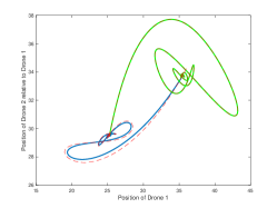
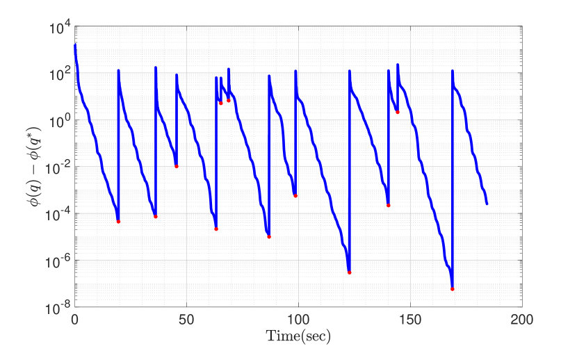
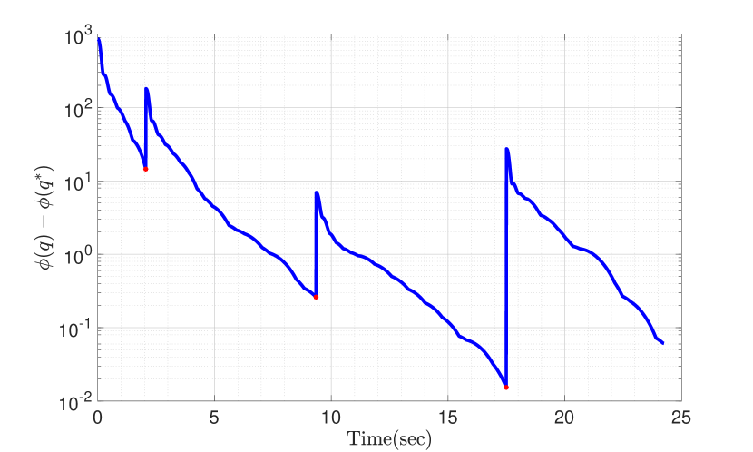
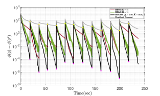
In this section, we give numerical examples for the application and the optimization method discussed in Sections V and IV-D respectively. In Figure 1, we consider a team of drones in a relay of distance , and we consider in order to demonstrate the -limit set. The blue line represents the position of the first drone (initial condition: distance of units from the data source), and the green line represents the position of a second drone relative to the first drone in the relay (initial condition: distance of units from the first drone). These two lines depict the -limit set of the ideal hybrid system given in (5). The red lines are created by allowing for the small dwell-time parameter . The switches satisfy the average dwell-time condition. Considering the switching behavior to be a small disturbance as in Theorem 2, we observe that the solutions converge to a small neighborhood of the -limit set of the ideal hybrid system. These observations agree with the results from Theorem 2. Figure 2(a) shows the decrease in the value of the objective function under the dynamics of the HiHBM algorithm applied to the problem (17) for drones in a relay of length , with the network-wide objective being for . Each is diagonal with eigenvalues i.i.d. uniform on , and each has its entries i.i.d. uniform on . The objective at each drone is , where is the distance from drone to drone , as described in Sec. V. We allow persistent switches satisfying average dwell time with . Figures 2(a) shows that HiHBM converges efficiently even as the objective switches persistently. Figure 2(b) shows the same example with fewer switches. In Figure 3, the gray line displays the gradient descent optimization. The red line demonstrates the convergence of the HBM optimization algorithm with and the green line demonstrates the same optimization algorithm with . The black line in Figure 3 shows the HiHBM optimization algorithm with a faster, more efficient convergence. The lower and upper-bound for HiHBM are and respectively. In Figure 3, we see the efficiency of the HiHBM algorithm that generates smaller errors in comparison with the simple gradient descent and the HBM method.
VII The proof of theorem 2
VII-A A new result on switching between constrained inclusions
Motivated by applications requiring persistent asset switches while optimizing, in this subsection we provide results on characterization of the asymptotic behavior that results from persistent switches among asymptotically stable differential inclusions with distinct equilibria. The switching signal is considered to satisfy an average dwell-time constraint as mentioned in the preliminaries IV-B.
VII-A1 Assumptions
We have two assumptions regarding the following family of differential inclusions parametrized by given as
| (23) |
Assumption 3.
For each , is outer semi-continuous, locally bounded relative to , and, for each , is non-empty and convex for all values of . Furthermore, the point is globally asymptotically stable for (23).
Assumption 4.
For each , the only solution to
| (24) |
with an initial value of is for all .
VII-B Extended Main Result
In this section, we adapt the results from [7] to the hybrid system . First, we establish boundedness for solutions to by claiming the following proposition and corollary.
Proposition 1.
If, for each , the system (23) is Lagrange stable, the hybrid system is Lagrange stable.
The proof of Proposition 1 follows the boundedness results from [7, Section 4.2] for the ideal hybrid system . As a consequence of Proposition 1 we have the following corollary.
Corollary 1.
If Assumption 3 holds then the hybrid system is Lagrange stable.
Using the definition of -limit set from [7], the rest of this section is devoted to the characterization of the -limit set of from a compact set denoted by . We use the definition of reachable sets from [7] and demonstrate the reachable set from with . Following the setting from [7], we define
| (25a) | ||||
| (25b) | ||||
This result follows from the following Lemmas.
Lemma 2.
If Assumption 3 holds then, for each compact set , .
Lemma 3.
VII-C Verifying that the systems in Section III satisfy the assumptions of Theorem 3
Theorem 4.
Proof.
Theorem 5.
Proof.
Proof of Theorem 2.
We now prove Theorem 2. Suppose Assumptions 1 and 2 hold. It follows from Theorems 4 and 5 that Assumptions 3 and 4 hold. From Theorem 3, it follows that the set in (25b) is semi-globally practically asymptotically stable for the system (4)-(6) embedded with an average dwell-time automaton as in (4) with respect to the parameter . Finally, according to Proposition 2, the set is the -limit set indicated in Theorem 2.
VIII Conclusions
We discussed the importance of enabling persistent switches of objective functions during an online execution of an optimization algorithm. The reason for these persistent switches is motivated by many engineering applications of convex optimization. We further extend the existing results of [7] on differential equations with multiple equilibria to differential inclusions with distinct multiple equilibria. We present the asset switches occurring in an optimization problem consisting of drones in a relay aiming for maximizing the signal strength. The asset switches are analyzed through the use of average dwell-time parameter which determines the rate of objective’s switching during the online HiHBM optimization. Hence, we establish semi-global practical asymptotic stability of a certain set with respect to this parameter. We characterize this set via Omega-limit sets.
References
- [1] E. G. Anderson Jr and K. Lewis, “A dynamic model of individual and collective learning amid disruption,” Organization Science, vol. 25, no. 2, pp. 356–376, 2014.
- [2] J. G. March, “Exploration and exploitation in organizational learning,” Organization science, vol. 2, no. 1, pp. 71–87, 1991.
- [3] W. Mei, N. E. Friedkin, K. Lewis, and F. Bullo, “Dynamic models of appraisal networks explaining collective learning,” IEEE Transactions on Automatic Control, vol. 63, no. 9, pp. 2898–2912, 2018.
- [4] H. Menouar, I. Guvenc, K. Akkaya, A. S. Uluagac, A. Kadri, and A. Tuncer, “UAV-enabled intelligent transportation systems for the smart city: Applications and challenges,” IEEE Communications Magazine, vol. 55, no. 3, pp. 22–28, 2017.
- [5] Y. Zhou, N. Cheng, N. Lu, and X. S. Shen, “Multi-UAV-aided networks: Aerial-ground cooperative vehicular networking architecture,” ieee vehicular technology magazine, vol. 10, no. 4, pp. 36–44, 2015.
- [6] I. Bekmezci, O. K. Sahingoz, and Ş. Temel, “Flying ad-hoc networks (fanets): A survey,” Ad Hoc Networks, vol. 11, pp. 1254–1270, 2013.
- [7] M. Baradaran and A. R. Teel, “Omega-limit sets and robust stability for switched systems with distinct equilibria,” IFAC Proceedings Volumes, vol. IFAC (International Federation of Automatic Control) World Congress in Berlin, 2020.
- [8] J. H. Le and A. R. Teel, “Hybrid heavy-ball systems: Reset methods for optimization with uncertainty,” to be published in Proc. American Control Conference, 2021.
- [9] T. Alpcan and T. Basar, “A stability result for switched systems with multiple equilibria,” Dynamics of Continuous, Discrete and Impulsive Systems Series A: Mathematical Analysis, vol. 17, pp. 949–958, 2010.
- [10] S. Veer, M. S. Motahar, and I. Poulakakis, “Generation of and switching among limit-cycle bipedal walking gaits,” in 56th IEEE Conference on Decision and Control, 2017, pp. 5827–5832.
- [11] G. Bianchin, J. Poveda, and E. Dall’Anese, “Online optimization of switched LTI systems using continuous-time and hybrid accelerated gradient flows,” to be published in Proc. American Control Conference, 2021.
- [12] R. Goebel, R. G. Sanfelice, and A. R. Teel, Hybrid Dynamical Systems. Princeton University Press, 2012.
- [13] J. P. Hespanha and A. S. Morse, “Stability of switched systems with average dwell-time,” in Proc. 38th IEEE Conference on Decision and Control, Sidney, Australia, 1999, pp. 2655–2660.
- [14] C. Cai, A. R. Teel, and R. Goebel, “Smooth Lyapunov functions for hybrid systems, Part II: (Pre)-asymptotically stable compact sets,” IEEE Transactions on Automatic Control, vol. 53, pp. 734–748, 2008.
- [15] R. Goebel, “A glimpse at pointwise asymptotic stability for continuous-time and discrete-time dynamics,” in Splitting Algorithms, Modern Operator Theory, and Applications. Springer, 2019, p. 243.
- [16] G. França, D. Robinson, and R. Vidal, “A nonsmooth dynamical systems perspective on accelerated extensions of ADMM,” arXiv:1808.04048, 2018.
- [17] A. Hauswirth, F. Dörfler, and A. Teel, “On the robust implementation of projected dynamical systems with anti-windup controllers,” in 2020 American Control Conference (ACC), 2020, pp. 1286–1291.
- [18] ——, “On the differentiability of projected trajectories and the robust convergence of non-convex anti-windup gradient flows,” IEEE Control Systems Letters, vol. 4, no. 3, pp. 620–625, 2020.
- [19] D. Bertsekas, Convex Optimization Theory, ser. Athena Scientific optimization and computation series. Athena Scientific, 2009.
- [20] R. Olfati-Saber, J. A. Fax, and R. M. Murray, “Consensus and cooperation in networked multi-agent systems,” Proceedings of the IEEE, vol. 95, no. 1, pp. 215–233, 2007.
- [21] E. Ghadimi, I. Shames, and M. Johansson, “Multi-step gradient methods for networked optimization,” IEEE Transactions on Signal Processing, vol. 61, no. 21, pp. 5417–5429, 2013.
- [22] Y. Nesterov, “Introductory lectures on convex optimization: A basic course,” Kluwer Academic Publishers, 2003.
- [23] A. Hauswirth, S. Bolognani, G. Hug, and F. Dörfler, “Timescale separation in autonomous optimization,” IEEE Transactions on Automatic Control, vol. 66, no. 2, pp. 611–624, 2021.
- [24] A. R. Teel, J. I. Poveda, and J. Le, “First-order optimization algorithms with resets and Hamiltonian flows,” in 2019 IEEE 58th Conference on Decision and Control (CDC), 2019, pp. 5838–5843.
- [25] I. Gutman and W. Xiao, “Generalized inverse of the Laplacian matrix and some applications,” Bulletin (Academie serbe des sciences et des arts. Classe des sciences mathematiques et naturelles. Sciences mathematiques), pp. 15–23, 2004.
- [26] E. P. Ryan, “An integral invariance principle for differential inclusions with applications in adaptive control,” SIAM J. Control Optim., vol. 36, no. 3, pp. 960–980, 1998.
- [27] A. Cherukuri and J. Cortés, “Distributed generator coordination for initialization and anytime optimization in economic dispatch,” IEEE Transactions on Control of Network Systems, vol. 2, no. 3, pp. 226–237, Sep. 2015.