Analyzing the Higgs-confinement transition with non-local operators on the lattice
Abstract
We study non-local operators for analyzing the Higgs-confinement phase transition in lattice gauge theory. Since the nature of the Higgs-confinement phase transition is topological, its order parameter is the expectation value of non-local operators, such as loop and surface operators. There exist several candidates for the non-local operators. Adopting the charge-2 Abelian Higgs model, we test numerical simulation of conventional ones, the Polyakov loop and the ’t Hooft loop, and an unconventional one, the Aharonov-Bohm phase defined by the Wilson loop wrapping around a vortex line.
I Introduction
In gauge theories coupled with fundamental matter, the Higgs phase and the confinement phase cannot be distinguished by any local order parameter because they have the same symmetry in the Ginzburg-Landau sense [1, 2, 3]. When the theory has topological order, the two phases are distinguishable by non-local order parameters and separated by a first-order phase transition. Otherwise, the two phases are continuously connected. A prominent example of the Higgs-confinement continuity is quantum chromodynamics (QCD) at nonzero density. Quarks form color singlet hadrons in the vacuum while quarks form diquark Cooper pairs with color-flavor locking in high density limit. The hadronic phase and the color-flavor locked phase have the same symmetry breaking pattern, and thus are expected to be smoothly connected without phase boundary. This is referred to as the quark-hadron continuity [4]. The quark-hadron continuity might be relevant for phenomenology of dense QCD matter, such as neutron star physics [5].
Non-local operators, such as loop and surface operators, play a key role in the Higgs-confinement phase transition. Well-known examples of the non-local operators are the Polyakov and ’t Hooft loops. These loops are (dis)order parameters of electric and magnetic confinement, respectively. In general, there is more than one order parameter for one phase transition. Among several candidates, a topological vortex [6, 7, 8, 9] and its Aharonov-Bohm phase [10, 11] were intensely discussed in the context of the quark-hadron continuity. Also, it was recently suggested that a correlation function on a vortex can distinguish the Higgs and confinement phases even if the transition is a smooth crossover [12]. Numerical simulation of lattice gauge theory is a powerful way to compute these non-local operators nonperturbatively. Some of them were already established and others were not. We need to deepen our understanding of their lattice implementation.
In this paper, we study the lattice implementation of a few non-local operators for analyzing the Higgs-confinement phase transition. We aim to showcase numerical analysis and to discuss practical difficulty etc. For this purpose, we should choose a simple gauge-Higgs model as a testing ground. We adopt the charge- Abelian Higgs model introduced by Fradkin and Shenker long ago [1] because its phase structure is well understood, thanks to many earlier works [13, 14, 15, 16, 17, 18, 19, 20]. Once we understand the implementation in this simple model, we can proceed to the next stage in forthcoming works; e.g., the SU(3) gauge-Higgs model, which is the Ginzburg-Landau theory of dense QCD.
The rest of the paper is organized as follows. We begin with a brief introduction of the Abelian Higgs model and the dual lattice in Sec. II. We discuss three non-local operators: the Polyakov loop in Sec. III, the ’t Hooft loop in Sec. IV, and the Aharonov-Bohm phase in Sec. V. All the equations are written in the lattice unit throughout the paper.
II Abelian Higgs model
We introduce the lattice formulation of the charge- Abelian Higgs model in dimensions. We employ the compact formulation with the unit-radius Higgs field. In the compact formulation, there are only two kinds of field variables: the Higgs field angle and the Abelian gauge field . The action takes the form
| (1) |
where is the unit lattice vector in direction and is the discretized field strength
| (2) |
This action is invariant under the local U(1) gauge transformation
| (3) | ||||
| (4) |
by an arbitrary function and the global transformation
| (5) |
The global symmetry exists only for multiple charge . We set in our numerical simulation.
The model has two parameters: the gauge coupling constant and the hopping parameter . These parameters control the phase of matter. The small regime is the confinement phase. The fields are strongly coupled and electrically charged particles are confined. The large and large regime is the Higgs phase. Since the hopping term is dominant, is frozen and Higgs condensation is induced. The large and small regime is the Coulomb phase. The vacuum is the weakly-coupled perturbative one. For , these three regimes are separated by the first-order phase transitions. In particular, the Higgs and confinement regimes are distinguishable by the global symmetry. This is in stark contrast to the model, where the global symmetry is absent and the confinement and Higgs regimes are smoothly connected without phase transition. The phase diagram of the charge- Abelian Higgs model was investigated in several previous lattice calculations. The calculation was first done with approximation [13], and then with exact U(1) for the specific heat [14], hysteresis [15], and magnetic monopole flow [16]. The location of phase boundaries was recently obtained with large lattice sizes [17]. The -dimensional model was also studied for and [18].
We also introduce the dual lattice for later convenience. The above model is defined on a four-dimensional hypercubic lattice with the volume . The dual lattice is also a four-dimensional hypercubic lattice with the volume . The dual sites are defined by the geometric centers of hypercubes of the original lattice. A -dimensional manifold on the original lattice has one-to-one correspondence to a -dimensional manifold on the dual lattice. We use a star symbol for describing dual manifolds. For example, an one-dimensional link penetrates a three-dimensional dual cube , a two-dimensional face intersects a two-dimensional dual face , and a three-dimensional cube is penetrated by an one-dimensional dual link . Magnetic objects, such as magnetic monopoles and vortices, are not elemental variables in the path integral but defined on the dual manifolds. The operators to create the magnetic objects are defined so as to act on the corresponding manifolds on the original lattice. The explicit operator constructions are demonstrated in Secs. IV and V. Note that the Abelian Higgs model can be rewritten and simulated by using dual variables [21, 22, 23], but we do not adopt such dual formulation in this work.
III Polyakov loop
The Polyakov loop is the most established order parameter of confinement-deconfinement phase transition [24]. Since the Polyakov loop is zero in the confinement phase and nonzero in the deconfinement phase, it is sometimes called a disorder parameter. The Polyakov loop was calculated in many studies of lattice gauge theory, mainly in SU() gauge theory. As for the charge- Abelian Higgs model, there is only one calculation and brief description [17]. Here we provide more detailed analysis.
We define the averaged Polyakov loop
| (6) |
from the Polyakov loop at the spatial coordinate
| (7) |
The expectation value
| (8) |
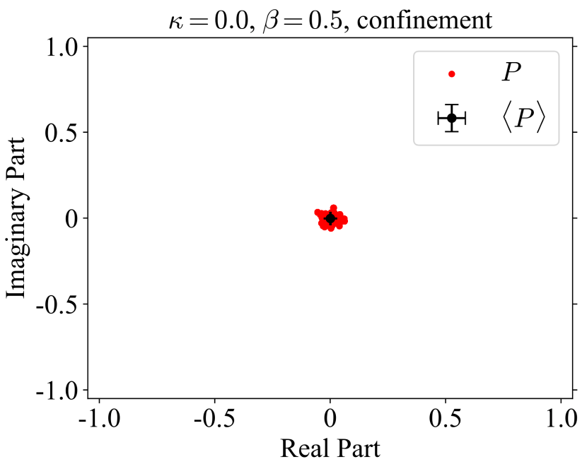
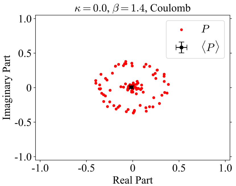
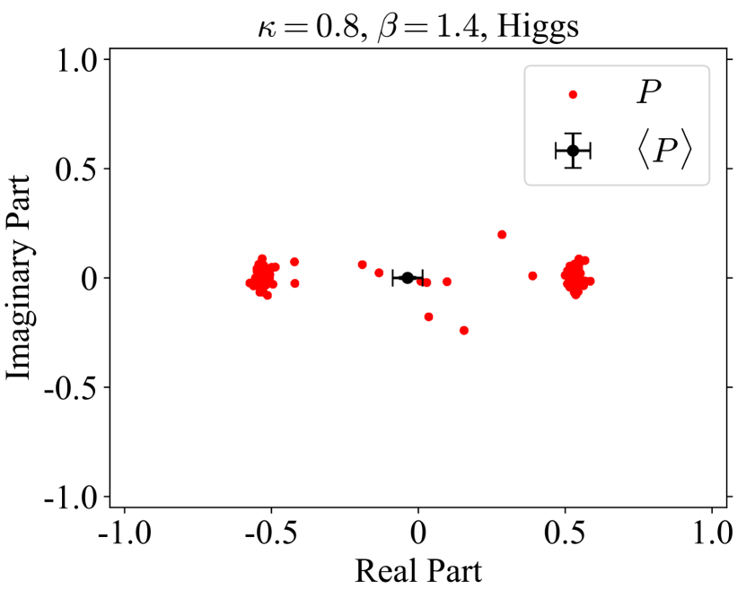
and are order parameters of spontaneous symmetry breaking. In numerical simulation, however, they are zero regardless of the phase because symmetry is not spontaneously broken in finite volume. The difference of the phase is seen in probability distribution. Figure 1 is scattering plots of the averaged Polyakov loop for each configuration. The number of gauge configuration is . The left panel is the case of and , which corresponds to the confinement phase of pure U(1) gauge theory. The distribution is very close to zero. For large , the system goes to the Coulomb phase. The distribution is away from zero and spreads into a circle, as shown in the middle panel. The circular distribution reflects the global U(1) symmetry in the pure gauge theory. The right panel corresponds to the Higgs phase. For , the hopping term in Eq. (6) breaks the global symmetry from U(1) to . When is very large, the hopping term restricts link variables to and the model is reduced to gauge theory. The distribution is concentrated in two minima on the real axis. The change of the distribution from U(1) to characterizes Coulomb-Higgs phase transition.
|
|
|
|
|
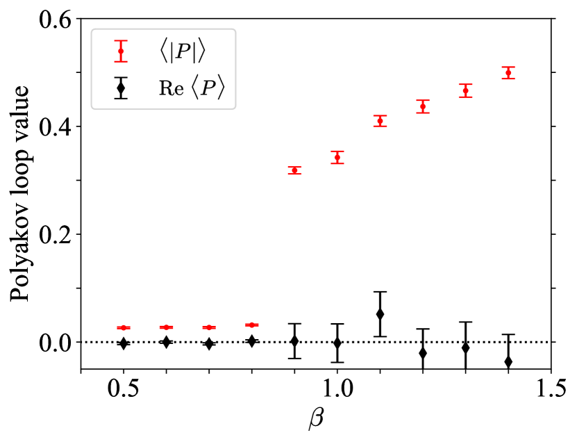
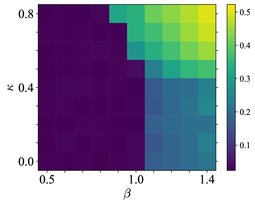
For determining transition points and drawing a phase diagram, we use instead of . (The non-averaged one cannot be used for this purpose because of in U(1) gauge theory. This is the reason why we take the spatial average in Eq. (6).) The results are shown in Fig. 2. The left panel shows the development of the Polyakov loop against at fixed . While is always zero, is nonzero and changes from small to large values. There is a sharp jump between and . This is the confinement-deconfinement phase transition and its critical coupling constant is at . The right panel is the phase diagram in - plane, where the values of are highlighted in different colors. The phase boundaries of the three phases are clearly seen. At , the system is pure U(1) gauge theory and the critical coupling constant is , which is consistent with pure gauge simulation [25, 26, 27]. The critical coupling constant gradually decreases as increases. The deconfinement phase is further decomposed into the Higgs and Coulomb regimes. They can be distinguished by the values of the Polyakov loop; the Higgs regime has larger values and the Coulomb regime has smaller values. This can be understood from the different distribution in Fig. 1. The Higgs-Coulomb phase transition occurs at -. All the results are consistent with previous studies [14, 15, 16, 17].
IV ’t Hooft loop
The ’t Hooft loop is dual to the Polyakov loop [28]. (In this paper, we consider the ’t Hooft loop encircling imaginary time direction.) The ’t Hooft loop is the worldline of a magnetic monopole while the Polyakov loop is the worldline of an electric charge. Since the ’t Hooft loop is nonzero in the confinement phase and zero in the Higgs phase, it is an order parameter of Higgs-confinement phase transition.
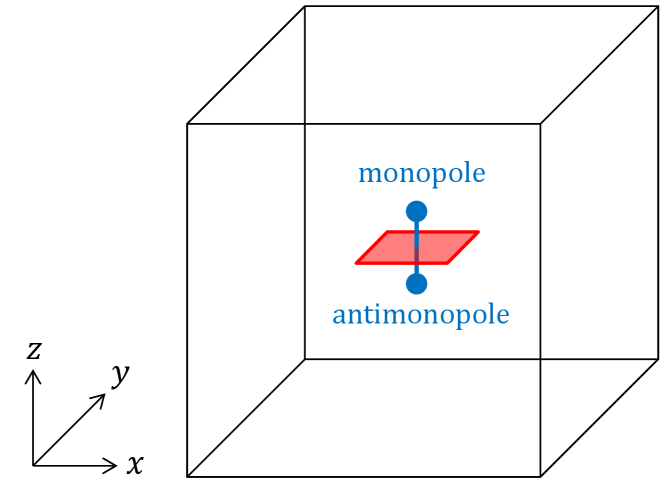
The lattice implementation of the ’t Hooft loop has been known since long ago [29, 30, 31] and applied to SU() gauge theory [32, 33, 34, 35, 36, 37, 38, 39, 40, 41]. The implementation generates the worldline of a magnetic monopole in dimensions. Here we apply it to the Abelian gauge theory in dimensions. In -dimensional case, the implementation generates the worldsheet of a magnetic string, not the worldline of a single monopole, because of extra spatial direction, i.e., direction. Let us consider the worldsheet on a two-dimensional dual surface in - plane. The surface has unit length in direction and wraps around direction. The corresponding magnetic string has unit length and its the endpoints are identified as a monopole and an antimonopole, as shown in the left panel of Fig. 3. We define the surface operator to create the worldsheet. The operation of multiplies a nontrivial element to all the plaquette variables intersecting . The expectation value of is given by
| (9) |
with the modified action
| (10) |
The surface is defined as a set of the - plaquettes intersecting . The expectation value is positive real. It is interpreted as , where is the free energy of a unit-length magnetic string, i.e., a monopole-antimonopole pair.
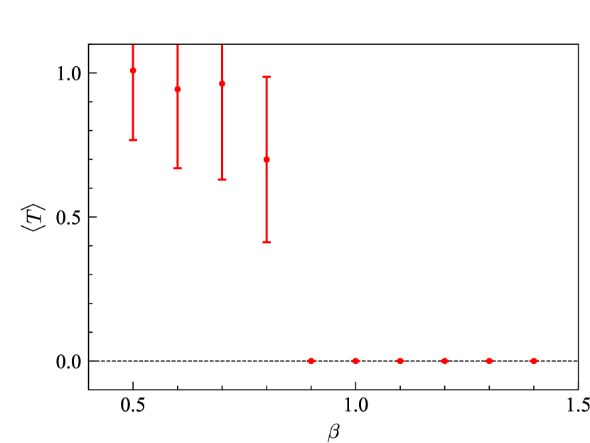
As shown in the right panel of Fig. 3, the simulation results clearly exhibit a jump of the first-order phase transition in spite of finite volume. The free energy of the monopole-antimonopole pair (two monopoles for ) is finite in the confinement phase and nearly infinite in the Higgs phase. The transition point - is consistent with that estimated from the Polyakov loop in the previous section. This indicate that the above formulation works well for analyzing the Higgs-confinement phase transition. Strictly speaking, however, the expectation value is not an order parameter of any symmetry. In dimensions, it is not the free energy of a single monopole but a monopole-antimonopole pair. The monopole-antimonopole pair has the same symmetry as the vacuum and its free energy will be large but finite even if a monopole is confined. The expectation value seems nearly zero but is not exactly zero in Fig. 3.
In practice, we computed Eq. (9) by the Monte Carlo sampling with sequential reweighting [38]. The computational cost of the reweighting method rapidly increases as the area of increases. The area of is proportional to and the length of the magnetic string in direction. Above we considered the magnetic string with unit length because the computational cost is small. The magnetic string wrapping around direction, i.e., without endpoints, can be considered and its free energy can be computed. This will show similar tendency although the cost is larger than ours.
V Aharonov–Bohm phase
The difference between the Higgs and confinement regimes also emerges in nontrivial correlation between non-local operators. It was recently conjectured that the two regimes are distinguished by the Aharonov–Bohm phase around a superfluid vortex [10]. This conjecture was analytically examined in the strong coupling and deep Higgs limits [11]. Lattice simulation will be necessary for full quantum examination. Here we formulate the lattice simulation of the Aharonov–Bohm phase and test it in the Abelian Higgs model. Note that the vortex in the Abelian Higgs model is not a global vortex of superfluid but a gauged vortex of superconductor. Although physics is different, the model can be used for testing formulation. The formulation is straightforwardly applicable to lattice gauge theories with a superfluid vortex, such as the non-Abelian Higgs model [42].
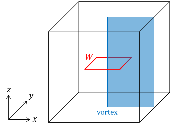
A vortex of the Higgs field is defined by nonzero circulation of . A vortex worldsheet can be generated by a cuboid operator on the dual lattice [43]. The setup is schematically depicted in the left panel of Fig. 4. Boundary conditions are open in and directions and periodic in and directions. Let denote the three-dimensional volume which lies from the center of the box to the boundary, and denote the links penetrating . The cuboid operator on is defined by multiplying the factor to the hopping terms in . This results in the circulation around the center of the box. The vortex exists at the center of the box and its worldsheet wraps around and directions. We define the charge- spatial Wilson loop
| (11) |
encircling the vortex, as shown in the figure. The path is a square on the - plane and its center is located at the vortex position. We computed the expectation value
| (12) |
with
| (13) |
Since the spatial Wilson loop is the trajectory of a charged particle, it picks up the Aharonov–Bohm phase when it encircles the vortex. We took the average of the translationally invariant loops in Eq. (12).
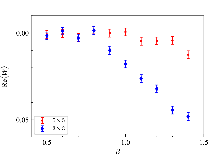
The right panel of Fig. 4 shows the real parts of the and Wilson loops. The imaginary parts are always zero in case of . The results of the loop are clear. The expectation value is negative in the Higgs phase. This corresponds to the non-trivial Aharonov–Bohm phase under coherent Higgs condensation. In the confinement regime, the expectation value is zero within statistical error and the Aharonov–Bohm phase is not calculable. The loop is qualitatively the same but not so clear due to statistical noise. In general, the expectation value of the Wilson loop is an exponentially damping function of loop size; the area law in the confinement regime and the perimeter law in the deconfinement regime. The signal to noise ratio drastically gets worse for larger loop. If one wants to take large loop limit, it will be computationally demanding. Although the asymptotic value of the Aharonov–Bohm phase is considered to be an order parameter, it will be hard to use it in practice.
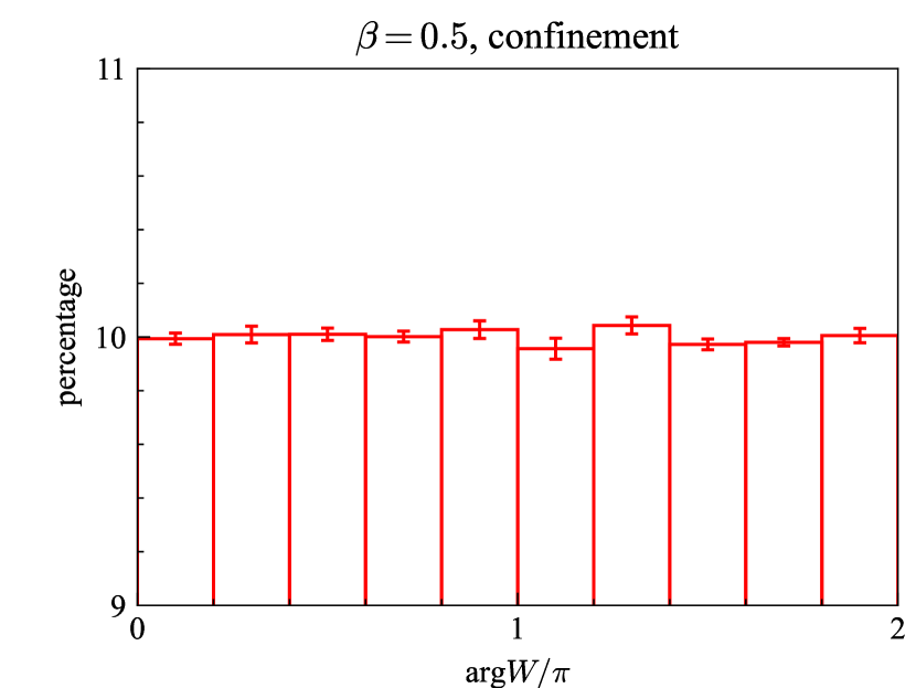
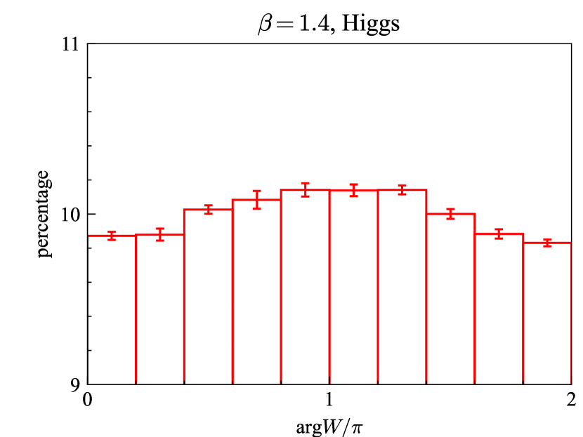
For looking more closely at the Aharonov–Bohm phase, let us quantify the angle of the Wilson loop. The expectation value is however ill-defined in quantum theory because it depends on the domain of argument. For example, when fluctuates around , if the argument is defined in , but if the argument is defined in . Instead, we here introduce probability distribution of . Because of in U(1) gauge theory, probability distribution of uniquely determines the expectation value. We generated gauge configurations, computed translationally invariant Wilson loops, and made one histogram, i.e., how many data exist in each domain of , from data. We repeated these steps for 10 independent sets of gauge configurations to evaluate statistical average and error. Thus, totally, we made a histogram from the data. As seen from the histograms in Fig. 5, the probability distribution changes between the Higgs and confinement regimes. In the confinement regime, the phase is random because of strong fluctuation of gauge fields. In the Higgs regime, the probability distribution has a peak at , but the peak is tiny, only about 0.1 %. This means that quantum fluctuation is still strong and semi-classical approximation is invalid. The probability distribution will go to delta function in classical limit, such as the deep Higgs limit .
Acknowledgements.
The authors thank Yui Hayashi for fruitful discussion. This work was supported by JSPS KAKENHI Grant No. 19K03841 and No. 24KJ0658, and JST SPRING Grant No. JPMJSP2108. The numerical simulations were partly carried out on SX-ACE in Osaka University.References
- Fradkin and Shenker [1979] E. H. Fradkin and S. H. Shenker, Phys. Rev. D 19, 3682 (1979).
- Banks and Rabinovici [1979] T. Banks and E. Rabinovici, Nucl. Phys. B 160, 349 (1979).
- Osterwalder and Seiler [1978] K. Osterwalder and E. Seiler, Annals Phys. 110, 440 (1978).
- Schäfer and Wilczek [1999] T. Schäfer and F. Wilczek, Phys. Rev. Lett. 82, 3956 (1999), arXiv:hep-ph/9811473 .
- Baym et al. [2018] G. Baym, T. Hatsuda, T. Kojo, P. D. Powell, Y. Song, and T. Takatsuka, Rept. Prog. Phys. 81, 056902 (2018), arXiv:1707.04966 [astro-ph.HE] .
- Alford et al. [2019] M. G. Alford, G. Baym, K. Fukushima, T. Hatsuda, and M. Tachibana, Phys. Rev. D 99, 036004 (2019), arXiv:1803.05115 [hep-ph] .
- Chatterjee et al. [2019] C. Chatterjee, M. Nitta, and S. Yasui, Phys. Rev. D 99, 034001 (2019), arXiv:1806.09291 [hep-ph] .
- Cherman et al. [2019] A. Cherman, S. Sen, and L. G. Yaffe, Phys. Rev. D 100, 034015 (2019), arXiv:1808.04827 [hep-th] .
- Hirono and Tanizaki [2019] Y. Hirono and Y. Tanizaki, Phys. Rev. Lett. 122, 212001 (2019), arXiv:1811.10608 [hep-th] .
- Cherman et al. [2020] A. Cherman, T. Jacobson, S. Sen, and L. G. Yaffe, Phys. Rev. D 102, 105021 (2020), arXiv:2007.08539 [hep-th] .
- Hayashi [2024] Y. Hayashi, Phys. Rev. Lett. 132, 221901 (2024), arXiv:2303.02129 [hep-th] .
- Hayata et al. [2024] T. Hayata, Y. Hidaka, and D. Kondo, Phase transition on superfluid vortices in Higgs-Confinement crossover (2024), arXiv:2411.03676 [hep-th] .
- Creutz [1980] M. Creutz, Phys. Rev. D 21, 1006 (1980).
- Bowler et al. [1981] K. C. Bowler, G. S. Pawley, B. J. Pendleton, D. J. Wallace, and G. W. Thomas, Phys. Lett. B 104, 481 (1981).
- Callaway and Carson [1982] D. J. E. Callaway and L. J. Carson, Phys. Rev. D 25, 531 (1982).
- Ranft et al. [1983] J. Ranft, J. Kripfganz, and G. Ranft, Phys. Rev. D 28, 360 (1983).
- Matsuyama and Greensite [2019] K. Matsuyama and J. Greensite, Phys. Rev. B 100, 184513 (2019), arXiv:1905.09406 [cond-mat.supr-con] .
- Bhanot and Freedman [1981] G. Bhanot and B. A. Freedman, Nucl. Phys. B 190, 357 (1981).
- Azcoiti and Tarancon [1986] V. Azcoiti and A. Tarancon, Phys. Lett. B 176, 153 (1986).
- Matsuyama [2021] K. Matsuyama, Phys. Rev. D 103, 074508 (2021), arXiv:2012.13991 [hep-lat] .
- Delgado Mercado et al. [2013a] Y. Delgado Mercado, C. Gattringer, and A. Schmidt, Comput. Phys. Commun. 184, 1535 (2013a), arXiv:1211.3436 [hep-lat] .
- Delgado Mercado et al. [2013b] Y. Delgado Mercado, C. Gattringer, and A. Schmidt, Phys. Rev. Lett. 111, 141601 (2013b), arXiv:1307.6120 [hep-lat] .
- Hayata and Yamamoto [2019] T. Hayata and A. Yamamoto, Phys. Rev. D 100, 074504 (2019), arXiv:1905.04471 [hep-lat] .
- Polyakov [1975] A. M. Polyakov, Phys. Lett. B 59, 82 (1975).
- Creutz et al. [1979] M. Creutz, L. Jacobs, and C. Rebbi, Phys. Rev. D 20, 1915 (1979).
- DeGrand and Toussaint [1980] T. A. DeGrand and D. Toussaint, Phys. Rev. D 22, 2478 (1980).
- Lautrup and Nauenberg [1980] B. E. Lautrup and M. Nauenberg, Phys. Lett. B 95, 63 (1980).
- ’t Hooft [1978] G. ’t Hooft, Nucl. Phys. B 138, 1 (1978).
- Mack and Petkova [1980] G. Mack and V. B. Petkova, Annals Phys. 125, 117 (1980).
- Ukawa et al. [1980] A. Ukawa, P. Windey, and A. H. Guth, Phys. Rev. D 21, 1013 (1980).
- Srednicki and Susskind [1981] M. Srednicki and L. Susskind, Nucl. Phys. B 179, 239 (1981).
- Billoire et al. [1981] A. Billoire, G. Lazarides, and Q. Shafi, Phys. Lett. B 103, 450 (1981).
- DeGrand and Toussaint [1982] T. A. DeGrand and D. Toussaint, Phys. Rev. D 25, 526 (1982).
- Kovacs and Tomboulis [2000] T. G. Kovacs and E. T. Tomboulis, Phys. Rev. Lett. 85, 704 (2000), arXiv:hep-lat/0002004 .
- Hart et al. [2000] A. Hart, B. Lucini, Z. Schram, and M. Teper, JHEP 11, 043, arXiv:hep-lat/0010010 .
- Hoelbling et al. [2001] C. Hoelbling, C. Rebbi, and V. A. Rubakov, Phys. Rev. D 63, 034506 (2001), arXiv:hep-lat/0003010 .
- Del Debbio et al. [2001] L. Del Debbio, A. Di Giacomo, and B. Lucini, Phys. Lett. B 500, 326 (2001), arXiv:hep-lat/0011048 .
- de Forcrand et al. [2001] P. de Forcrand, M. D’Elia, and M. Pepe, Phys. Rev. Lett. 86, 1438 (2001), arXiv:hep-lat/0007034 .
- de Forcrand and von Smekal [2002] P. de Forcrand and L. von Smekal, Phys. Rev. D 66, 011504 (2002), arXiv:hep-lat/0107018 .
- de Forcrand and Noth [2005] P. de Forcrand and D. Noth, Phys. Rev. D 72, 114501 (2005), arXiv:hep-lat/0506005 .
- de Forcrand et al. [2006] P. de Forcrand, C. Korthals-Altes, and O. Philipsen, Nucl. Phys. B 742, 124 (2006), arXiv:hep-ph/0510140 .
- Yamamoto [2018] A. Yamamoto, PTEP 2018, 103B03 (2018), arXiv:1804.08051 [hep-lat] .
- Shimazaki and Yamamoto [2020] T. Shimazaki and A. Yamamoto, Phys. Rev. D 102, 034517 (2020), arXiv:2006.02886 [hep-lat] .