∎
22email: h.ishizaka005@gmail.com 33institutetext: Kenta Kobayashi44institutetext: Graduate School of Business Administration, Hitotsubashi University, Kunitachi, Japan
44email: kenta.k@r.hit-u.ac.jp 55institutetext: Takuya Tsuchiya 66institutetext: Graduate School of Science and Engineering, Ehime University, Matsuyama, Japan
66email: tsuchiya@math.sci.ehime-u.ac.jp
Anisotropic interpolation error estimates using a new geometric parameter
Abstract
We present precise anisotropic interpolation error estimates for smooth functions using a new geometric parameter and derive inverse inequalities on anisotropic meshes. In our theory, the interpolation error is bounded in terms of the diameter of a simplex and the geometric parameter. Imposing additional assumptions makes it possible to obtain anisotropic error estimates. This paper also includes corrections to an error in Theorem 2 of our previous paper, “General theory of interpolation error estimates on anisotropic meshes” (Japan Journal of Industrial and Applied Mathematics, 38 (2021) 163-191).
Keywords:
Finite element Interpolation error estimates Anisotropic meshesMSC:
65D05 65N301 Introduction
Analyzing the errors of interpolations on -simplices is an important subject in numerical analysis. It is particularly crucial for finite element error analysis. Let us briefly outline the problems considered in this paper using the Lagrange interpolation operator.
Let . Let and be a reference element and a simplex, respectively, that are affine equivalent. Let us consider two Lagrange finite elements and with associated normed vector spaces and with , where is the space of polynomials with degree at most . For , we use the correspondences
where is an affine mapping. Let and be the corresponding Lagrange interpolation operators. Details can be found in Section 2.3.
We first consider the case in which . Let . For , let be a mesh of such as
where for . We denote for . If we set for , the mesh is said to be the uniform mesh. If we set for with a grading function , the mesh is said to be the graded mesh with respect to ; see BabSur94 . In particular, when (), the mesh is called the radical mesh. To obtain the Lagrange interpolation error estimates, we impose standard assumptions and specify that and such that
| (1) |
Under these assumptions, the following holds for any with :
| (2) |
The proof of this statement is standard; see ErnGue04 . When , it is possible to obtain optimal error estimates even if the scale is different for each element. When , the order of convergence of the interpolation operator may deteriorate.
We now consider the cases in which . Let be a bounded polyhedral domain. Let be a simplicial mesh of made up of closed -simplices, such as
with , where . For simplicity, we assume that is conformal. That is, is a simplicial mesh of without hanging nodes. Let be the reference element defined in Section 2 and be the affine mapping defined in Eq. (13). For any , it holds that . Under the standard assumptions and Eq. (1), the following holds for any with :
| (3) |
where is the measure of , the parameters and are defined in Eq. (50), and the parameter is as proposed in a recent paper IshKobTsu ; see Section 2.4 for a definition. The proof of estimate (3) can be found in Section 5. Compared with the one-dimensional case, the quantities and negatively affect the order of convergence and do not appear in Eq.(2). The two quantities and are considered in Section 7.1. As a mesh condition, the shape-regularity condition is widely used and well known. This condition states that there exists a constant such that
| (4) |
where is the radius of the inscribed ball of . Under this condition, it holds that
| (5) |
see Section 7.1.1. If condition (4) is violated (i.e., the simplex becomes too flat as ), the quantity
may diverge even when . The effect of the quantity on the interpolation error estimates is considered in Section 7.2.
In some cases, it is not necessary for condition (4) to hold to obtain Eq. (5). The shape-regularity condition can be relaxed to the maximum-angle condition, as stated in Eqs. (20) and (21), for both two-dimensional BabAzi76 and three-dimensional cases Kri92 . Anisotropic interpolation theory has also been developed ApeDob92 ; Ape99 ; CheShiZha04 . The idea of Apel et al. is to construct a set of functionals satisfying conditions (54), (55), and (56). The introduction of these functionals makes it possible to remove the quantity . Under the conditions of the maximum angle and coordinate system, anisotropic interpolation error estimates can then be deduced (e.g., see Ape99 ).
In contrast, this paper proposes anisotropic interpolation error estimates using the new parameter under conditions (54), (55), and (56) and Assumption 1; i.e., we derive the following anisotropic error estimate (Theorem B, in particular, Corollary 1):
| (6) |
where is defined in Eq. (12), is a multi-index, and is specified in Definition 3. Theorem B applies to interpolations other than the Lagrange interpolation, and the basis for the proof of Theorem B is the scaling argument described in Section 3.
Because the new geometric parameter is used in the interpolation error analysis, the coefficient used in the error estimation is independent of the geometry of the simplices, and the error estimations obtained may therefore be applied to arbitrary meshes, including very “flat” or anisotropic simplices. Furthermore, we are naturally able to consider the following geometric condition as being sufficient to obtain optimal order estimates (when ): there exists such that
| (7) |
Condition (7) appears to be simpler than the maximum-angle condition. Furthermore, the quantity can be easily calculated in the numerical process of finite element methods. Therefore, the new condition may be useful. A recent paper IshKobSuzTsu21 showed that the new condition is satisfied if and only if the maximum-angle condition holds. We expect the new mesh condition to become an alternative to the maximum-angle condition.
Furthermore, under Assumption 1, component-wise inverse inequalities can be deduced as (see Section 7.3):
In a previous paper IshKobTsu , the present authors developed new interpolation error estimations in a general framework and derived Raviart–Thomas interpolations on -simplices. However, the statement of Theorem 2 in IshKobTsu includes a mistake. That is, under standard assumptions, the quantity cannot be removed. We need to modify the statement of this theorem to correct this error. The current paper presents Theorems A (see Section 5) and B (see Section 6), which replace Theorem 2 of IshKobTsu . In Section 4, we explain the inaccuracies in the proof of Theorem 2 in IshKobTsu and describe how the results can be recovered using our Theorems A and B. Furthermore, the Babuška and Aziz technique is generally not applicable on anisotropic meshes in the proof of Theorem 3 in IshKobTsu . Details will be discussed in a coming paper Ish21 .
When there is no ambiguity, we use the notation and definitions given in IshKobTsu . Throughout this paper, denotes a constant independent of (defined later), unless specified otherwise. These values may change in each context. is the set of positive real numbers.
2 Strategy for constructing anisotropic interpolation theory
In standard interpolation theory, one introduces an affine mapping that connects the reference element to the mesh element. However, on anisotropic meshes, the interpolation errors may be overestimated. Therefore, our strategy is to divide the transformation into three affine mappings.
2.1 Standard positions of simplices
We recall (IshKobTsu, , Section 3). Let us first define a diagonal matrix as
| (8) |
2.1.1 Two-dimensional case
Let be the reference triangle with vertices , , and .
Let be the family of triangles
with vertices , , and .
We next define the regular matrices by
| (9) |
with parameters
For , let be the family of triangles
with vertices . We then have that and .
2.1.2 Three-dimensional case
Let and be reference tetrahedra with the following vertices:
- (i)
-
has the vertices , , , ;
- (ii)
-
has the vertices , , , .
Let , , be the family of triangles
with vertices
- (i)
-
, , , and ;
- (ii)
-
, , , and .
We next define the regular matrices by
| (10) |
with parameters
For , , let , , be the family of tetrahedra
with vertices
We then have , , and
In the following, we impose conditions for in the two-dimensional case and in the three-dimensional case.
Condition 1 (Case in which )
Let with the vertices () introduced in Section 2.1.1. We assume that is the longest edge of ; i.e., . Recall that and . We then assume that . Note that .
Condition 2 (Case in which )
Let with the vertices () introduced in Section 2.1.2. Let () be the edges of . We denote by the edge of that has the minimum length; i.e., . We set and assume that
Among the four edges that share an end point with , we take the longest edge . Let and be the end points of edge . Thus, we have that
Consider cutting with the plane that contains the midpoint of edge and is perpendicular to the vector . We then have two cases:
- (Type i)
-
and belong to the same half-space;
- (Type ii)
-
and belong to different half-spaces.
In each respective case, we set
- (Type i)
-
and as the end points of , that is, ;
- (Type ii)
-
and as the end points of , that is, .
Finally, we set . Note that we implicitly assume that and belong to the same half-space. In addition, note that .
Remark 1
Let be a conformal mesh. We assume that any simplex is transformed into such that Condition 1 is satisfied (in the two-dimensional case) or , , such that Condition 2 is satisfied (in the three-dimensional case) through appropriate rotation, translation, and mirror imaging. Note that none of the lengths of the edges of a simplex or the measure of the simplex is changed by the transformation.
Assumption 1
In anisotropic interpolation error analysis, we may impose the following geometric conditions for the simplex :
-
1.
If , there are no additional conditions;
-
2.
If , there exists a positive constant , independent of , such that . Note that if , this condition means that the order with respect to of coincides with the order of , whereas if , the order of may be different from that of .
2.2 Affine mappings
In our strategy, we adopt the following affine mappings.
2.3 Finite element generation
We follow the procedure described in (ErnGue04, , Section 1.4.1 and 1.2.1); see also (IshKobTsu, , Section 3.5).
For the reference element defined in Sections 2.1.1 and 2.1.2, let be a fixed reference finite element, where is a vector space of functions for some positive integer (typically or ) and is a set of linear forms such that
is bijective; i.e., is a basis for . Further, we denote by in the local (-valued) shape functions such that
Let be a normed vector space of functions such that and the linear forms can be extended to . The local interpolation operator is then defined by
| (14) |
It is obvious that
| (15) | |||
| (16) |
Let be the affine mapping defined in Eq. (13). For , we first define a Banach space of -valued functions that is the counterpart of and define a linear bijection mapping by
with the three linear bijection mappings
The triple is defined as
The triples and are similarly defined. These triples are finite elements and the local shape functions are , , and for , and the associated local interpolation operators are respectively defined by
| (17) | ||||
| (18) | ||||
| (19) |
Proposition 1
The diagrams
commute.
Proof
See, for example, (ErnGue04, , Proposition 1.62). ∎
2.4 New parameters
In a previous paper IshKobTsu , we proposed two geometric parameters,
Definition 2
The parameter is defined as
and the parameter is defined as
where denotes the edges of the simplex .
The following lemma shows the equivalence between and .
Lemma 1
It holds that
Furthermore, in the two-dimensional case, is equivalent to the circumradius of .
Proof
The proof can be found in (IshKobTsu, , Lemma 3). ∎
Remark 2
We set
As we stated in the Introduction, if the maximum-angle condition is violated, the parameter may diverge as on anisotropic meshes. Therefore, imposing the maximum-angle condition for mesh partitions guarantees the convergence of finite element methods Apeet21 . Reference BabAzi76 studied cases in which the finite element solution may not converge to the exact solution.
We now state the following theorem concerning the new condition.
Theorem 1
Proof
In the case of , we use the previous result presented in Kri91 ; i.e., there exists a constant such that
if and only if condition (20) is satisfied. Combining this result with being equivalent to the circumradius of , we have the desired conclusion. In the case of , the proof can be found in a recent paper IshKobSuzTsu21 . ∎
Lemma 2
It holds that
| (22a) | ||||
| (22b) | ||||
| (22c) | ||||
Furthermore, we have
| (23) |
Proof
The proof of (22b) can be found in (IshKobTsu, , (4.4), (4.5), (4.6), and (4.7)). The inequality (22a) is easily proved. Because , one easily finds that and recovers Eq. (22c). The proof of equality (23) is standard. ∎
For matrix , we denote by the -component of . We set . Furthermore, we use the inequality
| (24) |
3 Scaling argument
This section gives estimates related to a scaling argument corresponding to (ErnGue04, , Lemma 1.101). The estimates play major roles in our analysis. Furthermore, we use the following inequality (see (ErnGue04, , Exercise 1.20)). Let and , (), be real numbers. Then, we have that
| (25) |
Lemma 3
Let and . There exist positive constants and such that, for all and ,
| (26) |
with .
Proof
Lemma 4
Let and . Let be a multi-index with . Then, for any with and , it holds that
| (29) |
where is a constant that is independent of and . When , for any with and , it holds that
| (30) |
where is a constant that is independent of and .
Proof
Let . Because the space is dense in the space , we show that Eq. (29) holds for with and . From , we have that, for any multi-index ,
| (31) |
Through a change of variable, we obtain
| (32) |
From the standard estimate in (ErnGue04, , Lemma 1.101), we have
| (33) |
Inequality (29) follows from Eqs. (32) and (33) with Eq. (23).
We consider the case in which . A function belongs to the space for any . Therefore, it holds that for any and, from Eq. (25), we obtain
| (34) |
for the multi-index with . This implies that the function is in the space for each . Therefore, we have that . Taking the limit in Eq. (34) and using , we have
| (35) |
From the standard estimate in (ErnGue04, , Lemma 1.101), we have
| (36) |
We now introduce the following new notation.
Definition 3
We define a parameter , , as
For a multi-index , we use the notation
We also define and .
Definition 4
We define vectors , , as follows. If ,
and if ,
Furthermore, we define a directional derivative as
where is the orthogonal matrix defined in Eq. (12). For a multi-index , we use the notation
Note 1
Recall that
When , if Assumption 1 is imposed, there exists a positive constant , independent of , such that . Thus, if , we have
and if , for and , we have
Note 2
We use the following calculations in Lemma 5. For any multi-indices and , we have
Let with and . Then, for ,
and for ,
Lemma 5
Suppose that Assumption 1 is imposed. Let , with and . Let and be multi-indices with and . Then, for any with and , it holds that
| (37) |
where is a constant that is independent of and . Here, for and any positive real , .
Proof
Remark 3
In inequality (37), it is possible to obtain the estimates in by specifically determining the matrix .
Let , , and . Recall that
For with and , we have
Let . We define the matrix as
Because , we have
where the indices , and , must be evaluated modulo 2. Because , it holds that
We then have
where the indices , must be evaluated modulo 2.
We define the matrix as
We then have
which leads to
Using (25), we than have that
In this case, anisotropic interpolation error estimates cannot be obtained.
Note 3
We use the following calculations in Lemma 6. For any multi-indices and , we have
Let with , and . Then, for ,
and for ,
Lemma 6
Let , with , and . Let and be multi-indices with and . Then, for any with , , and , it holds that
| (39) |
where is a constant that is independent of and . Here, for and any positive real , .
4 Remarks on anisotropic interpolation analysis
We use the following Bramble–Hilbert-type lemma on anisotropic meshes proposed in (Ape99, , Lemma 2.1).
Lemma 7
Let with be a connected open set that is star-shaped with respect to a ball . Let be a multi-index with and be a function with , where , , , and . Then, it holds that
| (40) |
where depends only on , , , and , and is defined as
| (41) |
where is a given function with .
As explained in the Introduction, there exist some mistakes in the proof of Theorem 2 of IshKobTsu , and the statement is not valid in its original form. To clarify the following description, we explain the errors in the proof. Let be the reference element defined in Section 2.1.1. We set , , and . For , we set and . Inequality (29) yields
| (42) |
The coefficient appears on the right-hand side of Eq. (42). In (IshKobTsu, , Theorem 2), we wrongly claimed that could be canceled out. In fact, a further assumption is required for this. Using Eq. (41) and the triangle inequality, we have
We use inequality (40) to obtain the target inequality (IshKobTsu, , Theorem 2). To this end, we have to show that
| (43) |
However, this is unlikely to hold because Eqs. (14) and (16) yield
Using the classical scaling argument (see (ErnGue04, , Lemma 1.101)), we have
which does not include the quantity . Therefore, the quantity in Eq. (42) remains. Thus, the proof of (IshKobTsu, , Theorem 2) is incorrect.
To overcome this problem, we use some results from previous studies ApeDob92 ; Ape99 . That is, we assume that there exists a linear functional such that
Because the polynomial spaces are finite-dimensional, all norms are equivalent; i.e., because () is a norm on , we have that, for ,
Setting , we obtain Eq. (43). Using inequality (40) yields
and so inequality (42) together with Eq. (25) can be written as
| (44) |
Inequality (37) yields
| (45) |
Therefore, the quantity in Eq. (44) and the quantity in Eq. (45) cancel out.
5 Classical interpolation error estimates
The following embedding results hold.
Theorem
Let , , and . Let be a bounded open subset of . If is a Lipschitz set, we have that
| (46) |
Furthermore,
| (47) |
Proof
See, for example, (ErnGue04, , Corollary B.43, Theorem B.40), (ErnGue21a, , Theorem 2.31), and the references therein. ∎
Remark 4
Let and be such that
Then, it holds that .
Using the new geometric parameter , it is possible to deduce the classical interpolation error estimates; e.g., see (ErnGue04, , Theorem 1.103) and (ErnGue21a, , Theorem 11.13).
Theorem A
Let and assume that there exists a nonnegative integer such that
Let () be such that with the continuous embedding. Furthermore, assume that and such that and
| (48) |
Then, for any , it holds that
| (49) |
where is a positive constant that is independent of and , and the parameters and are defined as
| (50) |
6 Anisotropic interpolation error estimates
6.1 Main theorem
Theorem A can be applied to standard isotropic elements as well as some classes of anisotropic elements. If we are concerned with anisotropic elements, it is desirable to remove the quantity from estimate (49). To this end, we employ the approach described in Ape99 and consider the case of a finite element with and (Theorem B). However, one needs stronger assumptions to obtain the optimal estimate. When using finite elements that do not satisfy the assumptions of Theorem B (e.g., -bubble finite element), we have to use Theorem A. In these cases, it may not be possible to obtain optimal order estimates if the shape-regularity condition is violated.
Theorem B
Let be a finite element with the normed vector space and with . Let be a linear operator. Fix , , and such that , , and assume that the embeddings (46) and (47) with hold. Let be a multi-index with . We set . Assume that there exist linear functionals , , such that
| (54) | |||
| (55) | |||
| (56) |
For any , we set . If Assumption 1 is imposed, it holds that
| (57) |
where is a positive constant that is independent of and . Furthermore, if Assumption 1 is not imposed, it holds that
| (58) |
where is a positive constant that is independent of and .
Proof
The introduction of the functionals follows from Ape99 . In fact, under the same assumptions as made in Theorem B, we have (see (Ape99, , Lemma 2.2))
| (59) |
where , , and .
Example 1
6.2 Examples satisfying conditions (54), (55), and (56) in Theorem B
Corollary 1
Let be the Lagrange finite element with and for . Let be the corresponding local Lagrange interpolation operator. Let , , and be such that and
We set such that . Then, for all with , we recover Eq. (57) if Assumption 1 is imposed, and Eq. (58) holds.
Furthermore, for any with , it holds that
Proof
Setting , we define the nodal Crouzeix–Raviart interpolation operators as
Corollary 2
Let be the Crouzeix–Raviart finite element with and . Set . Let , , and be such that
Set such that . Then, for all with , we recover Eq. (57) if Assumption 1 is imposed, and Eq. (58) holds.
Furthermore, for any with , it holds that
Proof
For , we only introduce functionals satisfying Eqs. (54), (55), and (56) in Theorem B for each and .
Let . From the Sobolev embedding theorem, we have with , or , . Under this condition, we use
Let and (). We set . Then, we have that . We consider a functional
By an analogous argument, we can set a functional for the case .
Let and (). We first consider Type (i) in Section 2.1.2. That is, the reference element is . Here, form the canonical basis. We set and consider the functional
We now consider Type (ii) in Section 2.1.2. That is, the reference element is . We set and consider the functional
By an analogous argument, we can set functionals for cases .
When and , we can easily check that
∎
7 Concluding remarks
As our concluding remarks, we identify several topics related to the results described in this paper.
7.1 Good elements or not for ?
In this subsection, we consider good elements on meshes. Here, we define “good elements” on meshes as those for which there exists some satisfying Eq. (7). We treat a “Right-angled triangle,” “Blade,” and “Dagger” for , and a “Spire,” “Spear,” “Spindle,” “Spike,” “Splinter,” and ”Sliver” for , as introduced in Cheetal00 . We present the quantities and for these elements.
7.1.1 Isotropic mesh
We consider the following condition. There exists a constant such that, for any and any simplex , we have
| (62) |
Condition (62) is equivalent to the shape-regularity condition; see (BraKorKri08, , Theorem 1).
7.1.2 Anisotropic mesh: two-dimensional case
Let be a triangle. Let , , and . A dagger has one short edge and a blade has no short edge.
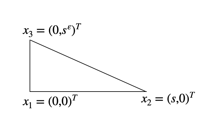
Example 2 (Right-angled triangle)
Let be the simplex with vertices , , and with . Then, we have that and ; i.e.,
In this case, the element is “good.”
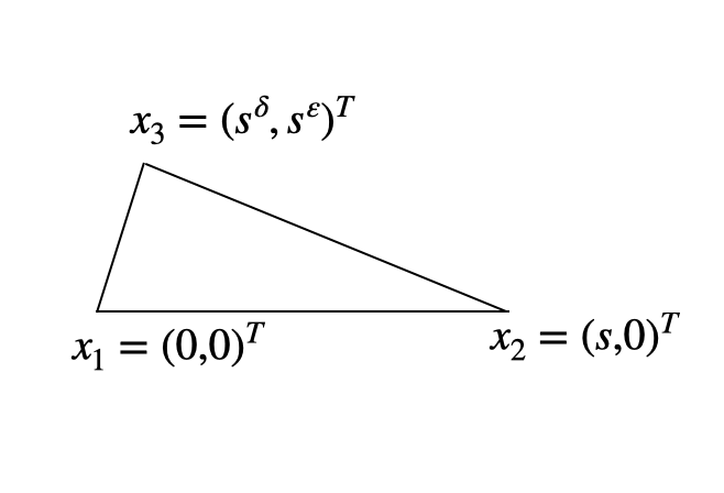
Example 3 (Dagger)
Let be the simplex with vertices , , and with . Then, we have that and ; i.e.,
In this case, the element is “good.”
Remark 6
In the above examples, holds. That is, the good element satisfies conditions such as .
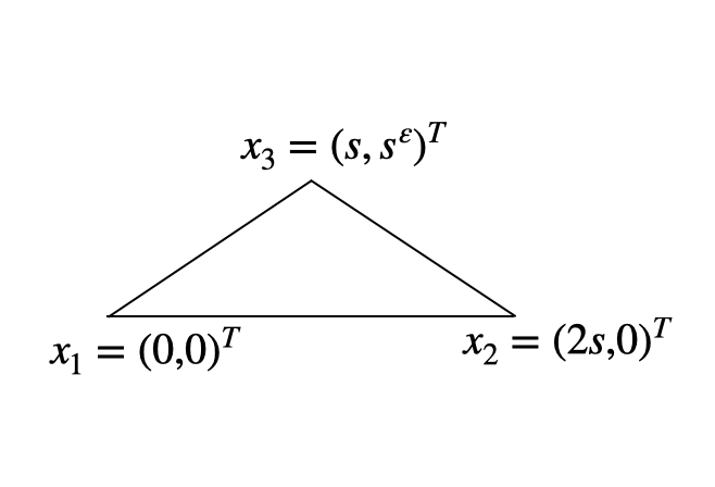
Example 4 (Blade)
Let be the simplex with vertices , , and with . Then, we have that ; i.e.,
In this case, the element is “not good.”
Example 5 (Dagger)
Let be the simplex with vertices , , and with . Then, we have that and ; i.e.,
In this case, the element is “not good.”
7.1.3 Anisotropic mesh: three-dimensional case
Example 6
Let be a tetrahedron. Let be the base of ; i.e., . Recall that
| (63) |
If the triangle is “not good,” such as in Examples 4 and 5, the quantity in Eq. (63) may diverge. In the following, we consider the case in which the triangle is “good.”
Assume that there exists a positive constant such that . For simplicity, we set , , and with . Then,
and because ,
If we set with , the triangle is the blade (Example 4). Then,
Thus, we have
In this case, the element is “not good.”
If we set with , the triangle is the dagger (Example 5). Then,
Thus, we have
In this case, the element is “not good.”
If we set with , the triangle is the dagger (Example 3). Then,
Thus, we have
In this case, the element is “good” and holds.
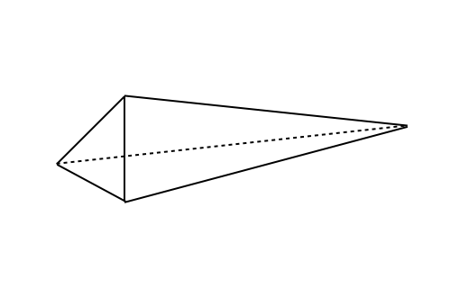
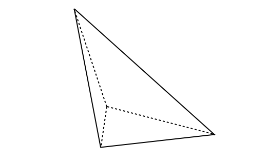
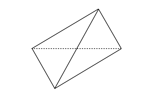
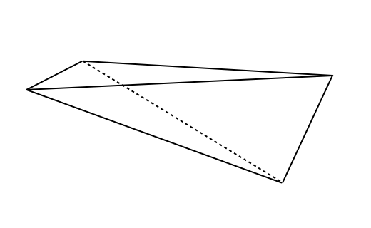
Example 7
In Cheetal00 , the spire has a cycle of three daggers among its four triangles. The splinter has four daggers. The spear and spike have two daggers and two blades as triangles. The spindle has four blades as triangles.
Remark 7
The above examples reveal that the good element satisfies conditions such as and .
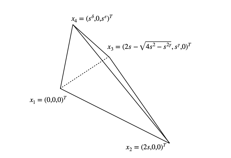
Example 8
Using an element called a Sliver, we compare the three quantities , , and , where the parameter denotes the circumradius of .
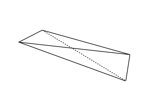
Let be the simplex with vertices , , , and (), where , . Let () be the edges of with . Recall that and
| 32 | 3.1250e-02 | 1.4033 | 6.7882e+01 | 3.4471e+01 | 5.0195e-01 |
|---|---|---|---|---|---|
| 64 | 1.5625e-02 | 1.4087 | 9.6000e+01 | 4.8375e+01 | 5.0098e-01 |
| 128 | 7.8125e-03 | 1.4115 | 1.3576e+02 | 6.8147e+01 | 5.0049e-01 |
| 32 | 3.1250e-02 | 5.6569 | 6.7882e+01 | 8.5513 | 5.0006e-01 |
|---|---|---|---|---|---|
| 64 | 1.5625e-02 | 8.0000 | 9.6000e+01 | 8.5184 | 5.0002e-01 |
| 128 | 7.8125e-03 | 1.1314e+01 | 1.3576e+02 | 8.5018 | 5.0000e-01 |
| 32 | 3.1250e-02 | 5.6569 | 3.8400e+02 | 3.4986e+01 | 1.4170 |
|---|---|---|---|---|---|
| 64 | 1.5625e-02 | 8.0000 | 7.6800e+02 | 4.8744e+01 | 2.0010 |
| 128 | 7.8125e-03 | 1.1314e+01 | 1.5360e+03 | 6.8411e+01 | 2.8288 |
In Table 1, the angle between and tends to as , and the simplex is “not good.” In Table 2, the angle between and tends to as , and the simplex is “good.” In Table 3, from the numerical results, the simplex is “not good.”
7.2 Effect of the quantity on the interpolation error estimates for
We now consider the effect of the factor .
7.2.1 Case in which
When , the factor may affect the convergence order. In particular, the interpolation error estimate may diverge on anisotropic mesh partitions.
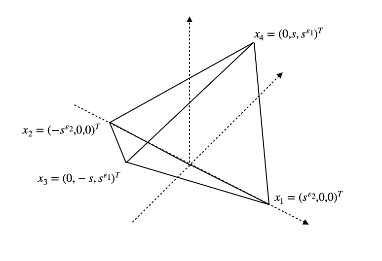
Let be the triangle with vertices , , for , , , and ; see Figure 2. Then,
Let , , , , and . Then, and Theorem B lead to
When (i.e., an isotropic element), we obtain
However, when (i.e., an anisotropic element), the estimate may diverge as . Therefore, if , the convergence order of the interpolation operator may deteriorate.
7.2.2 Case in which
We consider Theorem B. Let () be the local Lagrange interpolation operator. Let be such that , . Then, for any and , it holds that
| (64) |
Therefore, the convergence order is improved by .
We can perform some numerical tests to confirm this. Let and
- (I)
-
Let be the simplex with vertices , , , and (), and , . Then, we have that , , and ; i.e.,
From Eq. (64) with , , and , because , we have the estimate
Computational results for and are presented in Table 4.
Table 4: Error of the local interpolation operator () 64 1.5625e-02 2.4336e-08 128 7.8125e-03 1.5209e-09 4.00 256 3.9062e-03 9.5053e-11 4.00 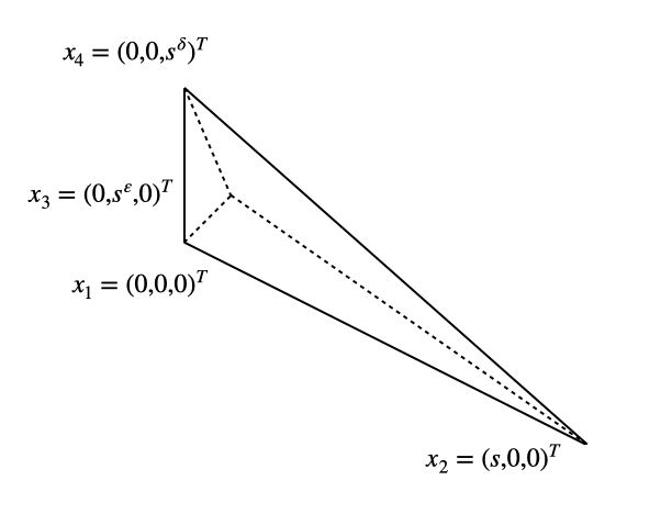
Figure 11: Case in which , Example (I) - (II)
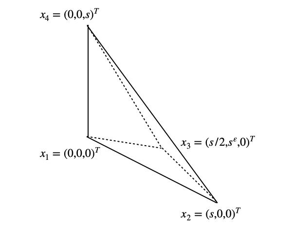
-
Let be the simplex with vertices , , , and () and , . Then, we have that , , and ; i.e.,
From Eq. (64) with , , and , because , we have the estimate
Computational results for are presented in Table 5.
Table 5: Error of the local interpolation operator () 64 1.5625e-02 1.9934e-04 1.0206e-01 128 7.8125e-03 7.0477e-05 1.50 1.0206e-01 0 256 3.9062e-03 2.4917e-05 1.50 1.0206e-01 0
7.3 Inverse inequalities
This section presents some limited results for the inverse inequalities. The results are only stated; the proofs can be found in Ish22 .
Lemma 8
Let with . If Assumption 1 is imposed, there exist positive constants , , independent of and , such that, for all ,
| (65) |
Remark 8
Theorem D
Let with . Let be a multi-index such that . If Assumption 1 is imposed, there exists a positive constant , independent of and , such that, for all ,
| (67) |
Acknowledgements.
We would like to thank the anonymous referees and the editor of the journal for the valuable comments.References
- (1) Apel, Th.: Anisotropic finite elements: Local estimates and applications. Advances in Numerical Mathematics. Teubner, Stuttgart, (1999)
- (2) Apel, Th., Nicaise, S., Schöberl, J.: Crouzeix–Raviart type finite elements on anisotropic meshes. Numer. Math. 89, 193-223 (2001)
- (3) Apel, Th, Dobrowolski, M.: Anisotropic interpolation with applications to the finite element method. Computing 47, 277-293 (1992)
- (4) Apel, T., Eckardt, L., Hauhner, C., Kempf, V.: The maximum angle condition on finite elements: useful or not? , PAMM (2021)
- (5) Babuška, I., Aziz, A.K.: On the angle condition in the finite element method. SIAM J. Numer. Anal. 13, 214-226 (1976)
- (6) Babuška, I., Suri, M.: The and - versions of the finite elements method, basic principles and properties. SIAM Review. 36, 578-632 (1994)
- (7) Brandts, J., Korotov, S., Kíek, M.: On the equivalence of regularity criteria for triangular and tetrahedral finite element partitions. Comput. Math, Appl. 55, 2227-2233 (2008)
- (8) Brenner, S.C., Scott, L.R.: The Mathematical Theory of Finite Element Methods, Third Edition. Springer Verlag, New York (2008)
- (9) Chen, S., Shi, D., Zhao, Y.: Anisotropic interpolation and quasi-Wilson element for narrow quadrilateral meshes. IMA Journal of Numerical Analysis, 24, 77-95 (2004)
- (10) Cheng, S. -W., Dey, T. K., Edelsbrunner, H., Facello, M. A., Teng, S. -H.: Sliver Exudation. J. ACM, 47, 883-904 (2000)
- (11) Ciarlet, P. G.: The Finite Element Method for Elliptic problems. SIAM, New York (2002)
- (12) Dekel, S., Leviatan, D.: The Bramble–Hilbert Lemma for Convex Domains, SIAM Journal on Mathematical Analysis 35 No. 5, 1203-1212 (2004)
- (13) Ern, A., Guermond, J.L.: Theory and Practice of Finite Elements. Springer Verlag, New York (2004)
- (14) Ern, A., Guermond, J.L.: Finite Elements I: Galerkin Approximation, Elliptic and Mixed PDEs. Springer Verlag, New York (2021)
- (15) Ishizaka, H.: Anisotropic Raviart–Thomas interpolation error estimates using a new geometric parameter. https://arxiv.org/abs/2110.02348, (2021)
- (16) Ishizaka, H.: Anisotropic interpolation error analysis using a new geometric parameter and its applications. Ehime University, Ph. D. thesis, (2022)
- (17) Ishizaka, H., Kobayashi, K., Tsuchiya, T.: General theory of interpolation error estimates on anisotropic meshes. Jpn. J. Ind. Appl. Math., 38 (1), 163-191 (2021)
- (18) Ishizaka, H., Kobayashi, K., Tsuchiya, T.: Crouzeix–Raviart and Raviart–Thomas finite element error analysis on anisotropic meshes violating the maximum-angle condition. Jpn. J. Ind. Appl. Math., 38 (2), 645-675 (2021)
- (19) Ishizaka, H., Kobayashi, K., Suzuki, R. Tsuchiya, T.: A new geometric condition equivalent to the maximum angle condition for tetrahedrons, Computers & Mathematics with Applications 99, 323-328 (2021)
- (20) Kíek, M.: On semiregular families of triangulations and linear interpolation. Appl. Math. Praha 36, 223-232 (1991)
- (21) Kíek, M.: On the maximum angle condition for linear tetrahedral elements. SIAM J. Numer. Anal. 29, 513-520 (1992)