Andrei Galiautdinov
Department of Physics and Astronomy,
University of Georgia, Athens, Georgia 30602, USA
ag@physast.uga.edu
(September 18, 2025)
Abstract
We generalize the classic calculations by Rytova and Keldysh of screened Coulomb
interaction in semiconductor thin films to systems with anisotropic permittivity tensor.
Explicit asymptotic expressions for electrostatic potential energy of interaction in
the weakly anisotropic case are found in closed analytical form. The case of strong
in-plane anisotropy, however, requires evaluation of the inverse Fourier transform of
, which, at present, remains unresolved.
is modified under the minimal number of microscopic assumptions.
In what follows, we provide the general expression for the Fourier image of
the anisotropic potential in momentum space, and analytically
work out in real space the weakly anisotropic case only. Interested readers
are invited to improve on that calculation by exploring the strongly anisotropic
scenario.
II General considerations
The electrostatic potential energy of interaction between charges and
located at and (, )
inside an anisotropic semiconductor film of thickness surrounded
by two isotropic media with dielectric constants and
is given by (see Appendix for derivation and Fig. 6;
compare with Rytova1967 ; keldysh1979coulomb )
(2)
with
(3)
where
(4)
and the axes of the coordinate system coincide with the principal axes
of the film’s permittivity tensor,
.
In the most interesting for practical applications scenario,
, and,
for distances , the main contribution to the integral in
(2) comes from satisfying .
Under these conditions,
, ,
and, with the dependence on and disappearing, we get the two-dimensional
form of the interaction,
(5)
At this point it is convenient to introduce two “screening” lengths,
(6)
characterizing polarizability of the film in the and directions,
respectively, and write the interaction (5) in the form
(7)
where is the dielectric function, formally defined by
(8)
which generalizes the standard isotropic result cudazzo2011dielectric .
In Ref. berkelbach2013theory , for the case of surrounding vacuum in
the isotropic scenario, the authors have numerically verified that the
screening length of a monolayer can be calculated with good accuracy
on the basis of Eq. (6)
provided the dielectric contrast is large and the relevant dielectric constant
of the monolayer is the in-plane component of the permittivity
tensor of the bulk material. We take that as an indication that the Keldysh model
is a good approximation to realistic experimental situations and hypothesize
that its anisotropic generalization proposed here should work reasonably well
even for samples of monolayer thickness.
The problem thus reduces to the calculation of a two-dimensional Fourier integral,
(9)
with .
To that end, working in polar coordinates, we write,
(10)
where , is the angle between the position vector
and the positive -axis, as shown in Fig. 6,
(11)
and
(12)
with playing the role of the anisotropy parameter; the greater
the , the greater the anisotropy, with corresponding to the isotropic
case.
Without loss of generality, we may assume that
, and thus .
Then, since , we have .
Taking into account the well-known Fourier series expansion
mikhlin1964integral ,
(13)
and using the fact that
,
we get for the -integral in (11) the
asymptotic multipole series,
where and are the Bessel functions of the first kind.
III Weak anisotropy
In a rather straightforward manner (for a better approach see
Sec. IV), assuming and
treating as a small parameter
in (II), we get, in lowest order,
(15)
and, thus,
(16)
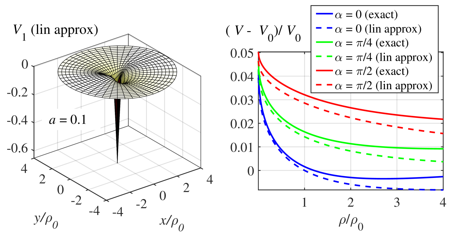
Figure 1:
Graphs of in units of
,
and , with , in the weakly anisotropic case, calculated
on the basis of Eqs. (III) and (18)
and direct numerical integration in Eq. (II).
Performing the remaining -integration we find,
(17)
where
(18)
is the standard Keldysh-Rytova result, and
(19)
is the linear correction whose graph is shown in Fig. 1
(assuming ). In the above, various and
denote the Struve and Neumann functions, respectively.
For , or ,
we get
(20)
(21)
where is the Euler constant.
Since , the excitonic ground state
energy in this case experiences a first order shift,
(22)
where is the unperturbed axially symmetric ground state
wave function.
On the other hand, for , or
,
Eqs. (18) and (III) reproduce the
standard Coulomb asymptotics,
(23)
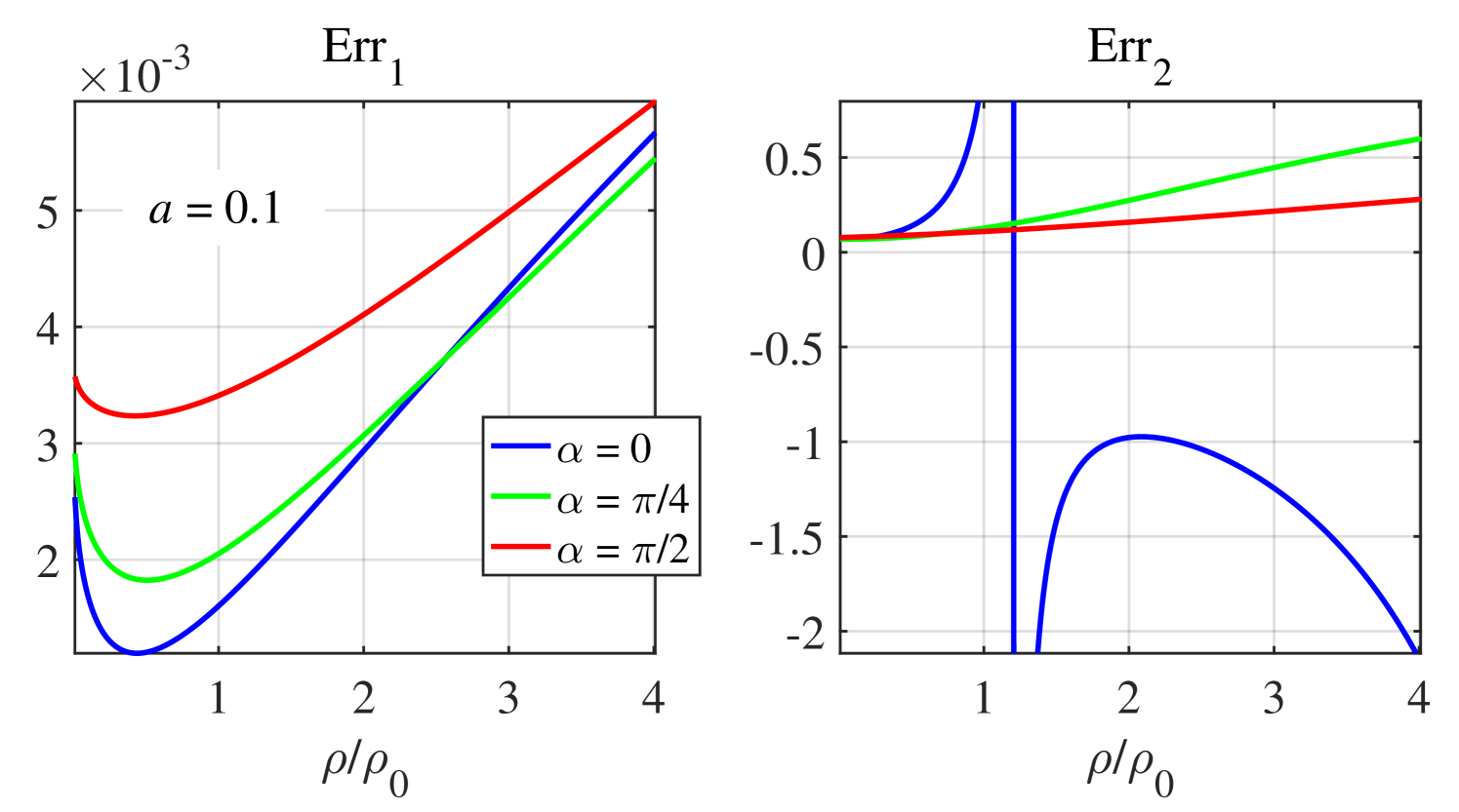
Figure 2:
Graphs of the relative errors defined in Eqs. (24)
and (25). The vertical asymptote (in blue) is at the
point with , for which (exact Keldysh value);
compare with Fig. 1.
To get a sense of the error involved in this linear approximation, we define two
relative errors by
(24)
and
(25)
respectively, with .
Here, is calculated on the basis of
Eqs. (18) and (III),
and is found by direct numerical integration of the double integral
in (II). The corresponding results are summarized in
Fig. 2. Notice that for all the error is greatest
for points with . The error is particularly troublesome,
as the blue curve clearly indicates.
IV Weak anisotropy: Renormalized Keldysh interaction
A better linear approximation can be achieved by “renormalizing” the zeroth
order Keldysh contribution, , as follows: we re-write the monopole term in
(II) as shown below,
(26)
and expand everything in square brackets to linear (leading!) order in .
The potential then becomes
is the corresponding linear correction consisting of a linear monopole and a linear
dipole contributions, Fig. 3.
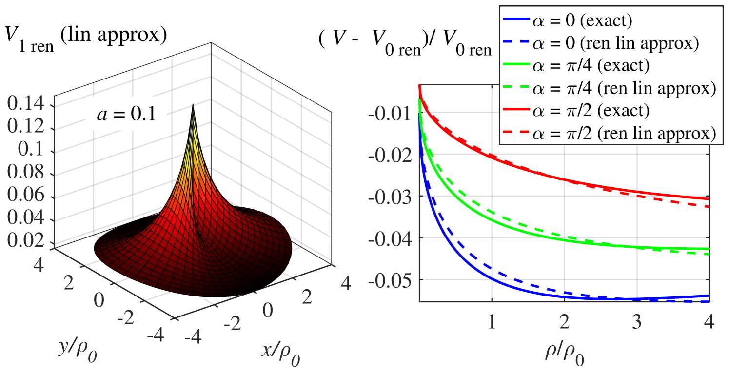
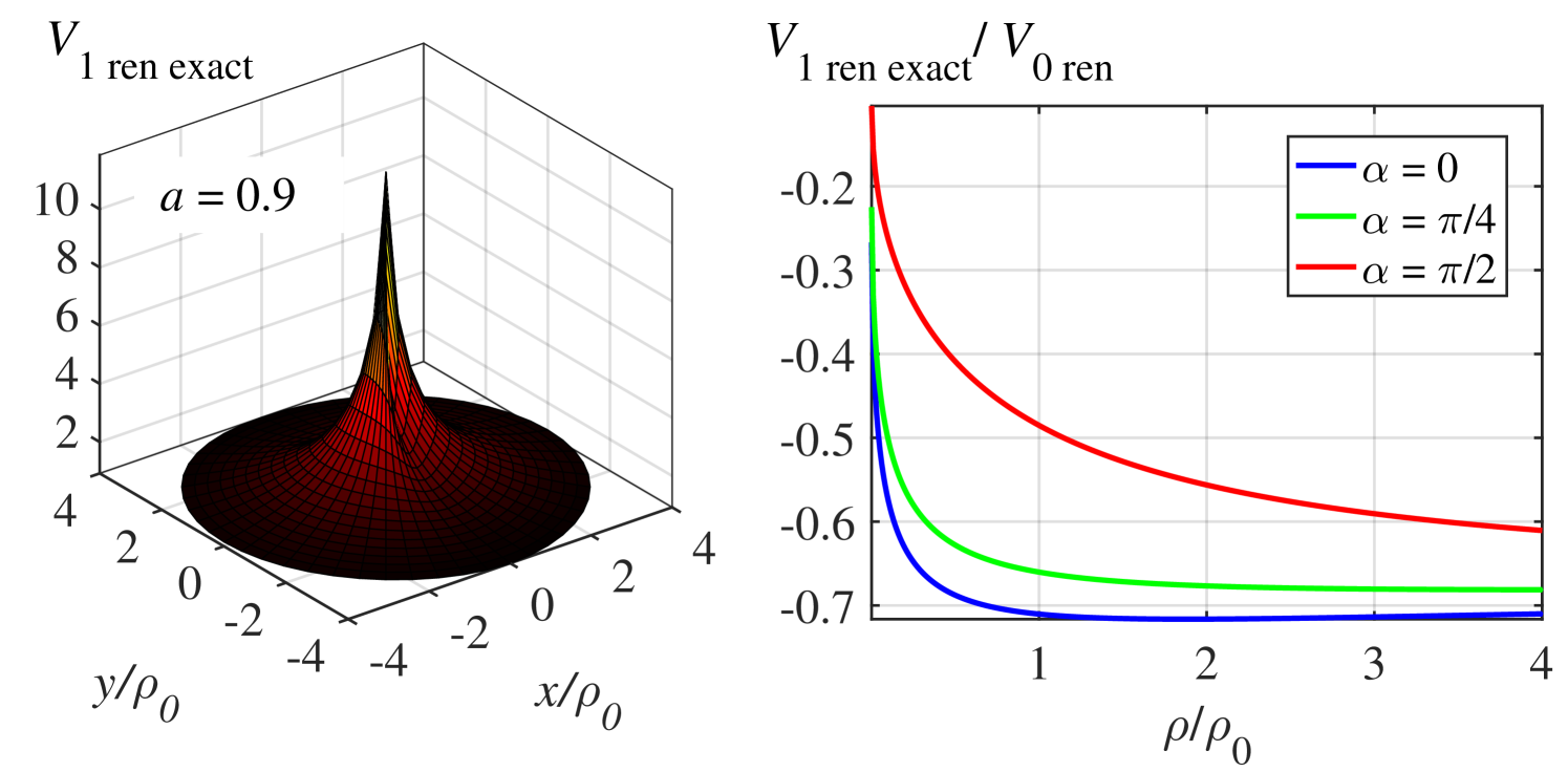
Figure 3:
Graphs of in units of
,
and , with ,
in the weakly anisotropic case, calculated
on the basis of Eqs. (29) and (IV)
and direct numerical integration in Eq. (II).
Compare with Fig. 1.
Now in the limit we get
(31)
and a perfectly reasonable first order correction
(32)
which does not contain the logarithmic term. The excitonic ground state
energy in this case undergoes a simple first order shift,
(33)
Notice that our renormalization procedure eliminates logarithmic terms in all orders
of the monopole perturbation, not just the first one.
For example, keeping the second order monopole contribution in square brackets in
Eq. (26) would add the term
(34)
to the potential in (28), which in the limit is just
(35)
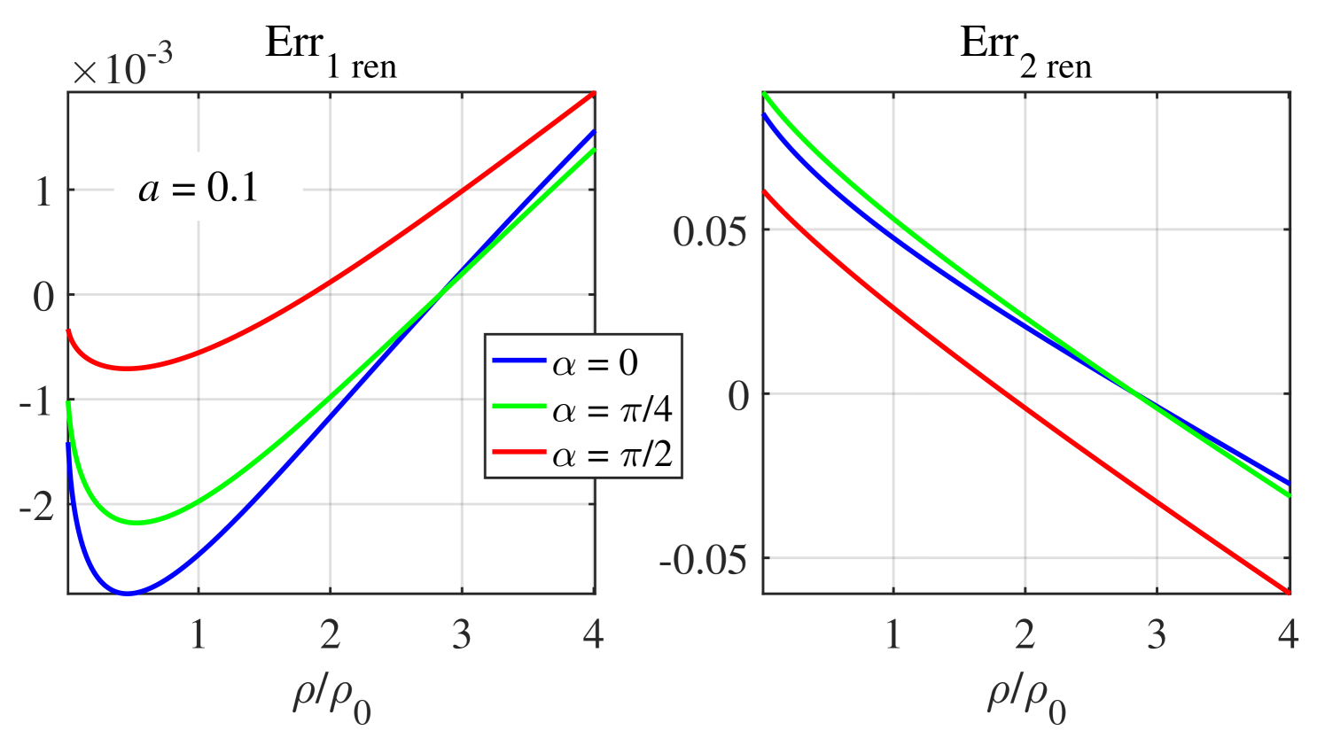
Figure 4:
Graphs of the relative errors defined in Eqs. (36)
and (37). Compare with Fig. 2.
Figure 5:
Graphs of in units of
and , with , in
the strongly anisotropic case (calculated numerically
on the basis of Eqs. (II)
and (29)).
Returning to the linear approximation (28), we again define two
relative errors,
(36)
and
(37)
with and
.
The corresponding numerical results presented in Fig. 4 show
that our revised approximation scheme is indeed superior to the one used in
Sec. III.
Finally, we also performed numerical simulations in the extreme anisotropic regime,
as shown in Fig. 5. In this case, the “correction”
becomes comparable to , and the linear approximation breaks down.
V Summary
The classic Keldysh-Rytova formula for screened Coulomb interaction in semiconductor
thin films has been generalized by taking into account the anisotropy of the layer’s
dielectric permittivity tensor. The Fourier image of the anisotropic potential in
momentum space, as well as the linear correction to the isotropic potential in
real space, have been worked out in closed analytical form. The case of strong
in-plane anisotropy, however, remains unresolved due to the appearance
of the function (see Eqs. (11) and (II)),
whose explicit analytical expression is not known.
Acknowledgements.
The author thanks Robert Zaballa for useful discussions.
APPENDIX: Momentum space representation
Following Rytova1967 and keldysh1979coulomb ,
we consider a geometry in which
the anisotropic semiconductor film occupies the region of space ,
as shown in Fig. 6. The half-space (the substrate) is filled
with an isotropic medium whose dielectric constant is ,
while the half-space with an isotropic medium whose dielectric
constant is .
We are assuming that the axes of the coordinate system
coincide with the principal axes of the film’s dielectric permittivity tensor.
The electrostatic potential at point
due to charge located at satisfies in regions 1, 2,
and 3 (the film) the following system of equations:
(38)
(39)
(40)
with the boundary conditions at the interfaces,
(41)
(42)
and the boundary conditions at the two infinities,
(43)
Figure 6:
Left: Semiconductor film geometry; the axes
coincide with the principal axes of the dielectric permittivity tensor of the film,
.
Right: Mutual orientation of vectors and used
in Eq. (5).
Fourier transforming,
(44)
and substituting into (38), (39), and (40), we get
the following equations for the corresponding Fourier components,
(45)
(46)
(47)
where
(48)
Conditions at infinity, (43), combined with Eqs. (45)
and (46) give
(1)
P. Cudazzo, C. Attaccalite, I. V. Tokatly, and A. Rubio,
“Strong Charge-Transfer Excitonic Effects and the Bose-Einstein Exciton Condensate
in Graphane,”
Phys. Rev. Lett. 104, 226804 (2010).
(2)
P. Cudazzo, I. V. Tokatly, and A. Rubio,
“Dielectric screening in two-dimensional insulators: Implications for excitonic
and impurity states in graphane,”
Phys. Rev. B 84, 085406 (2011).
(3)
A. Chernikov, T. C. Berkelbach, H. M. Hill, A. Rigosi, Y. Li, O. B. Aslan,
D. R. Reichman, M. S. Hybertsen, and T. F. Heinz,
“Exciton Binding Energy and Nonhydrogenic Rydberg Series in Monolayer WS2,”
Phys. Rev. Lett. 113, 076802 (2014).
(4)
T. Low, R. Roldán, H. Wang, F. Xia, P. Avouris, L. M. Moreno, and F. Guinea,
“Plasmons and Screening in Monolayer and Multilayer Black Phosphorus,”
Phys. Rev. Lett. 113, 106802 (2014).
(5)
X. Wang, A. M. Jones, K. L. Seyler, V. Tran, Y. Jia, H. Zhao, H. Wang,
L. Yang, X. Xu and F. Xia,
“Highly anisotropic and robust excitons in monolayer black phosphorus,”
Nature Nanotechnology 10, 517 (2015).
(6)
A. Chaves, T. Low, P. Avouris, D. Cakir, and F. M. Peeters,
“Anisotropic exciton Stark shift in black phosphorus,”
Phys. Rev. B 92, 155311 (2015).
(7)
S. Latini, T. Olsen, and K. S. Thygesen,
”Excitons in van der Waals heterostructures: The important role of dielectric screening,”
Phys. Rev. B 92, 245123 (2015).
(8)
T. G. Pedersen, S. Latini, K. S. Thygesen, H. Mera and B. K. Nikolić,
“Exciton ionization in multilayer transition-metal dichalcogenides,”
New J. Phys. 18 (2016).
(9)
M. L. Trolle, T. G. Pedersen and V. Véniard,
“Model dielectric function for 2D semiconductors including substrate
screening,”
Nature Sci. Rep. 7, 39844 (2017).
(10)
A. Hichri, I. B. Amara, S. Ayari and S. Jaziri,
“Dielectric environment and/or random disorder
effects on free, charged and localized excitonic states in monolayer WS2,”
J. Phys.: Condens. Matter 29, 435305 (2017).
(11)
M. Szyniszewski, E. Mostaani, N. D. Drummond, and V. I. Fal’ko,
“Binding energies of trions and biexcitons in two-dimensional semiconductors
from diffusion quantum Monte Carlo calculations,”
Phys. Rev. B 95, 081301(R) (2017).
(12)
E. Mostaani, M. Szyniszewski, C. H. Price, R. Maezono,
M. Danovich, R. J. Hunt, N. D. Drummond, V. I. Fal’ko,
“Diffusion quantum Monte Carlo study of excitonic complexes in two-dimensional
transition-metal dichalcogenides,”
Phys. Rev. B 96, 075431(2017).
(13)
L. S. R. Cavalcante, A. Chaves, B. Van Duppen, F. M. Peeters, and
D. R. Reichman,
“Electrostatics of electron-hole interactions in van derWaals heterostructures,”
Phys. Rev. B 97, 125427 (2018).
(14)
Sh. Niu, G. Joe, H. Zhao, Y. Zhou, T. Orvis, H. Huyan,
J. Salman, K. Mahalingam, B. Urwin, J. Wu, Y. Liu,
T. E. Tiwald, S. B. Cronin, B. M. Howe, M. Mecklenburg, R. Haiges,
D. J. Singh, H. Wang, M. A. Kats and J. Ravichandran,
“Giant optical anisotropy in a quasi-one-dimensional crystal,”
Nature Photonics 12, 392 (2018).
(15)
Sh. Niu, H. Zhao, Y. Zhou, H. Huyan, B. Zhao, J. Wu, S. B. Cronin , H. Wang,
and J. Ravichandran,
“Mid-wave and Long-Wave Infrared Linear Dichroism in a Hexagonal Perovskite
Chalcogenide,”
Chem. Mater. 30 (15), 4897 (2018).
(16)
N. S. Rytova,
“Screened potential of a point charge in a thin film,”
Vestn. Mosk. Univ. Fiz. Astron. 3, 30 (1967).
(17)
L. V. Keldysh,
“Coulomb interaction in thin semiconductor and semimetal films,”
Pis’ma Zh. Eksp. Teor. Fiz. 29, 716 (1979)
[JETP Lett., 29, 658 (1979)].
(18)
L. V. Keldysh, “Excitons in Semiconductor-Dielectric Nanostructures,”
Phys. Stat. Sol. (a) 164, 3 (1997).
(19)
T. C. Berkelbach, M. S. Hybertsen, D. R. Reichman,
“Theory of neutral and charged excitons in monolayer transition metal
dichalcogenides,”
Phys. Rev. B 88, 045318 (2013).
(20)
S. G. Mikhlin, Integral Equations, Second Revised Edition (Pergamon Press,
1964).