Anisotropy of electronic stopping power in graphite

Jessica Halliday Theory of Condensed Matter, Cavendish Laboratory, University of Cambridge, J. J. Thomson Ave, Cambridge CB3 0HE, United Kingdom Emilio Artacho Theory of Condensed Matter, Cavendish Laboratory, University of Cambridge, J. J. Thomson Ave, Cambridge CB3 0HE, United Kingdom CIC Nanogune and DIPC, Tolosa Hiribidea 76, 20018 San Sebastian, Spain Ikerbasque, Basque Foundation for Science, 48011 Bilbao, Spain

(August 2, 2025)

Abstract

The rate of energy transfer from ion projectiles onto the electrons of a solid target is hard to determine experimentally in the velocity regime between the adiabatic limit and the Bragg peak. First-principles simulations have lately offered relevant new insights and quantitative information for prototypical homogeneous materials. Here we study the influence of structural anisotropy on electronic stopping power with time-dependent density functional theory simulations of a hydrogen projectile in graphite. The projectile traveled at a range of angles and impact parameters for velocities between 0.1 and 1.4 a.u., and the electronic stopping power was calculated for each simulation. After validation with average experimental data, the anisotropic crystal structure was found to have a strong influence on the stopping power, with a difference between simulations parallel and perpendicular to the graphite plane of up to 25%, more anisotropic than expected based on previous work. The velocity dependence at low velocity displays clear linear behavior in general, except for projectiles traveling perpendicular to graphitic layers, for which a threshold-like behavior is obtained. For projectiles traveling along graphitic planes metallic behavior is observed with a change of slope when the projectile velocity reaches the Fermi velocity of the electrons.

pacs:

PACS:

I Introduction

Stopping power is the rate of energy loss along the path of a charged particle as it passes through matter. Stopping power is of interest in a wide range of areas, from nuclear power generation to medical applications Was (2007); Begg et al. (2011). Two mechanisms of energy loss are involved: nuclear stopping, due to the interaction of the projectile with the nuclei of the target, and electronic stopping, from the interaction of the projectile with the electrons of the target. This work focusses on the electronic stopping power ( $S_{e}$ ), which dominates at high projectile velocities.

Most of modern electronics is based on materials and heterostructures grown along well-controlled crystalline directions, a trend that appears to continue in the brave new world of two-dimensional materials, heterostructures and devices based on them. A good characterisation of the orientation dependence of radiation effects would appear quite relevant for ascertaining on resilience of such devices. Of particular interest is the velocity regime in which projectiles are fast enough for non-adiabatic effects to be important, but not so fast so as to become insensitive the structure, pointing to the scale of a few tenths of an atomic unit of velocity (1 a.u. $=c/137$ ). Previous studies in various materials have investigated anisotropy in $S_{e}$ in thin films, particularly at higher energies Eisen et al. (1972); Dygo et al. (1994); dos Santos et al. (1997) However knowledge of the effect of structural anisotropy at velocities of a few tenths of a.u. is still very limited given the difficulties in obtaining experimental information in this rangeKäferböck et al. (1997); Softky (1961); Seltzer and Berger (1982); Crawford (1990); Shukri et al. (2016).

Experimentally $S_{e}$ is difficult to measure directly, particularly at low velocities where nuclear stopping is also significant; simulations, however, allow $S_{e}$ to be directly accessed. Echenique $et\ al.$ Echenique et al. (1981, 1986) used density functional theory to calculate electronic stopping power in jellium, capturing non-linear effects and replicating experimental results not captured in linear-response theory calculations Ferrell and Ritchie (1977); Lindhard (1954), also giving rise to derived simulations, including the use of first principles techniques for the indirect calculation of $S_{e}$ (for reviews see Echenique et al. (1990); Sigmund (2014)). Direct, real-time simulations of the electronic stopping process have also been performed during the last decade using a time-dependent tight binding description of the electronic structure and dynamics, coupled to nuclear dynamics within an Ehrenfest approach Mason et al. (2007); Race et al. (2010), providing interesting and rich qualitative insights, especially powerful given the large system size and long time scale affordable with an empirical tight-binding scheme. In recent years time-dependent density functional theory (TDDFT) has been used to investigate stopping power from first principles in bulk materials of different kinds (metals, semiconductors, insulators) Krasheninnikov et al. (2007); Pruneda et al. (2007); Zeb et al. (2012); Correa et al. (2012); Zeb et al. (2013); Ojanperä et al. (2014); Caro et al. (2015); Schleife et al. (2015); Ullah et al. (2015); Caro et al. (2017); Bubin et al. (2012); Lee, Cheng-Wei and Schleife, André (2018); Yost et al. (2017). First principles simulation of electronic stopping has successfully reproduced many experimental features not captured by other theoretical or simulation methods.

A prototypical material with a highly anisotropic layered structure is graphite, composed of weakly bonded layers of strongly hexagonally bonded carbon atoms, resulting in a high degree of inhomogeneity in many properties Chung (2002). A major use of graphite is as a moderator in the nuclear power industry, to absorb and slow down the neutrons generated by the nuclear fission processes, in order to control the rate of fission within a nuclear reactor. The stopping power of graphite is thus of intrinsic interest, in addition to its position as a simple and strongly anisotropic material, and was therefore chosen as the target material in this work. The velocity dependence of $S_{e}$ is addressed in the work, with an emphasis on its variation with trajectory.

A previous work on anisotropy of stopping power in graphite is a theoretical study by Crawford Crawford (1990), using linear response theory based on the Cazaux model Cazaux (1970) for the optical constants of graphite parallel and perpendicular to the graphitic layers. Crawford’s work calculated, for higher energy projectiles, a similar relationship between the incident angle of the projectile and the $S_{e}$ as this work. They found a small anisotropy of $S_{e}$ , with a variability of around 10% for projectile velocities between 2 and 20 a.u.. More recent work by Shukri, Bruneval and Reining Shukri et al. (2016) used linear response TDDFT to predict the random electronic stopping power in various materials. They found a similar small anisotropy of up to 3% between the $S_{e}$ along the in-plane and out-of-plane axes of graphite, for velocities between 0 and 4 a.u.. Previous experimental work by Yagi $et\ al.$ Yagi et al. (2004) was unable to direct projectiles between the graphitic layers, illustrating the usefulness of simulations to investigate the structural anisotropy of $S_{e}$ .

II Method

II.1 Simulation details

Simulations were carried out using the real-time TDDFT implementation Tsolakidis et al. (2002); Ullah et al. (2019) of the SIESTA method Soler et al. (2002); Artacho et al. (2008). The Kohn-Sham orbitals are expanded in a finite basis set of numerical atomic orbitals, with the valence electrons of graphite and the projectile represented by a double- $\zeta$ polarised basis set. The core electrons have been replaced by norm-conserving pseudopotentials using the Troullier-Martins scheme Froyen et al. ; Troullier and Martins (1991). Core electrons are known not to interact in stopping processes at low velocities Shukri et al. (2016); Ullah et al. (2018). The details of both the basis set and the pseudopotentials are specified in the Appendix. The local density approximation (LDA) was used for the exchange-correlation functional evaluation using the Ceperley-Alder results for the homogeneous electron liquid Ceperley and Alder (1980), in the parameterisation of Perdew and Zunger Perdew and Zunger (1981), considering adiabatic time dependence of the exchange-correlation functional.

The ground state of the system is calculated with the projectile stationary at its initial position in the graphite box. Subsequent TDDFT simulations evolve the electronic wavefunctions according to the time-dependent Kohn-Sham equation Kohn and Sham (1965); Runge and Gross (1984) as the projectile moves at a constant velocity through the box. The forces on all atoms are held as zero throughout the time-dependent simulation, so that energy transfer only takes place through inelastic scattering to the system electrons. This prevents any contribution from nuclear stopping and enables the $S_{e}$ to be directly calculated at a single velocity for each simulation. The electronic stopping is the average gradient of the total energy of the electronic system as a function of the path length of the projectile Ullah et al. (2015). The error bars in the $S_{e}$ presented in the figures refer to uncertainty in fitting to the slope.

Projectiles moved the full length of the simulation cell, 13.4 Å. Simulations were carried out using projectiles with velocities between 0.1 and 1.4 a.u.Pietsch et al. (1976). The time-dependent Kohn-Sham equations were integrated using a Crank-Nicholson integrator as in Ref. Tsolakidis et al., 2002 adapted to the changing basis and Hilbert space by using a Löwdin transformation as proposed by Sankey and Tomkoff Tomfohr and Sankey and analysed in Ref. 48. See the Appendix for further details of convergence testing.

II.2 Simulation trajectories

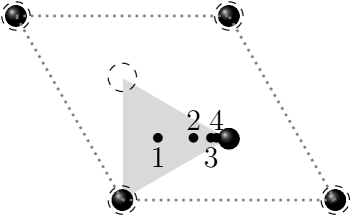
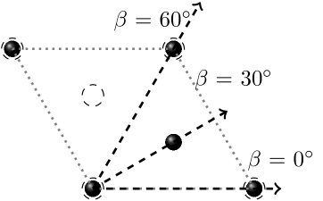
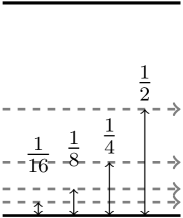
Simulations were run with a combination of the following parameters: the velocity of the projectile varied between 0.1 and 1.4 a.u., and the initial angle of the projectile relative to the $c$ axis of the graphite, $\alpha$ , varied between $0^{\circ}$ and $90^{\circ}$ as shown in Figure 1b. For simulations of projectiles moving parallel to the graphitic layers, the projectiles moved at an angle $\beta$ relative to the $a$ axis, at $0^{\circ}$ and $30^{\circ}$ , with checks at $60^{\circ}$ and $90^{\circ}$ as shown in Figure 2a, and moving at distances of $\frac{1}{2},\frac{1}{4},\frac{1}{8}$ and $\frac{1}{16}$ of the spacing between the layers from the closest graphitic layer, as shown in Figure 2b.

Concerning the charge state of the projectile, previous TDDFT work on electronic stopping has been carried out with both ions and atoms Ojanperä et al. (2014); Krasheninnikov et al. (2007); Ullah et al. (2015); Zeb et al. (2013). In this type of simulation, the use of a proton or a H atom only changes the simulation by one electron in the supercell (out of 129). The extent to which the proton drags an electron in its wake is defined dynamically, and the established stationary state is independent of the initial charge state of the projectile. After the initial transient, essentially the same state evolves regardless of whether it was initially H⁺ or H, in comparison with other methods in which the charge state is defined by handEchenique et al. (1990). The calculations presented here had 129 electrons in the simulation box, thereby defining an overall neutral system. The calculations were spin-polarised due to the odd number of electrons in the system.

III Results and Discussion

III.1 Validation

In order to validate the simulations, the results are compared in Figure 3 with experimental data from work by Käferböck $et\ al.$ Käferböck et al. (1997). In the velocity range covered by the experimental data, electronic stopping dominates the overall stopping power, so the simulations of electronic stopping are directly comparable to the Käferböck data. The Rutherford backscattering experiment used protons with an energy of between 20 and 80 keV, corresponding to projectile velocities between 1 and 1.7 a.u., with a target of highly ordered pyrolytic graphite, although they did not provide angle resolution for the measured $S_{e}$ . They consider ion trajectories in all directions.

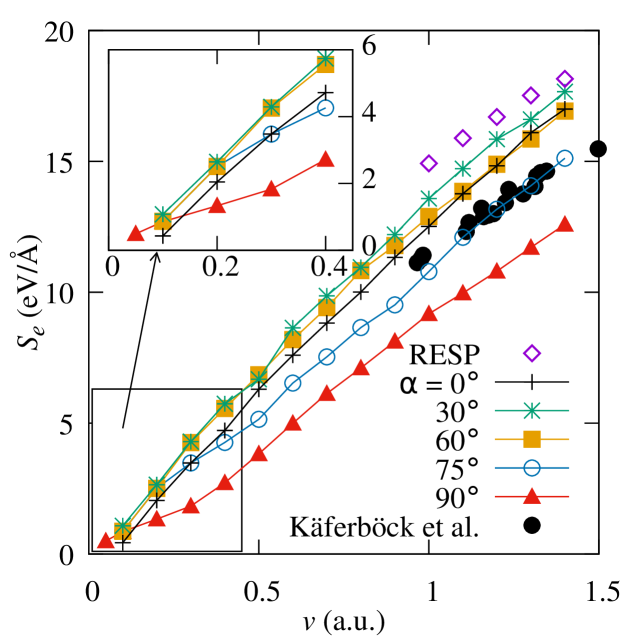
In Figure 3, the agreement between experiment and theory is clear, with the experimental observations lying within the simulation range defined by different trajectories. The experimental stopping power is closest to that of the higher angle simulations, $\alpha=60^{\circ}$ - $75^{\circ}$ . As channelling directions were avoided in the experiments, it is likely that trajectories close to $\alpha=90^{\circ}$ contribute little to the experimental averaging. See a similar consideration in the work of Schleife $et\ al.$ Schleife et al. (2015) for a proton moving in aluminium. In order to compare the simulations to the experimental data in more detail, a model of the distribution of projectile trajectories would be needed to calculate an average $S_{e}$ for a particular velocity, which involves non-trivial assumptions on the actual trajectories in experimental settings. $S_{e}$ gradually diminishes toward the minimum at $\alpha=90^{\circ}$ , starting at around $\alpha=50-60^{\circ}$ where a slight maximum appears, especially at low velocities.

III.2 Dependence on $\alpha$

Figure 3 shows the expected overall linear dependence of $S_{e}$ in the displayed velocity range, with a slow downward bending as velocity increases towards the $S_{e}$ maximum related to the Bragg peak, which in graphite is at $\sim$ 1.9 a.u. Deasy (1994). The curve for $\alpha=90^{\circ}$ is clearly different, however, corresponding to trajectories parallel to graphitic planes. As Figure 4 shows more clearly, the electronic stopping power decreases significantly at all velocities between $\alpha=60^{\circ}$ and $\alpha=90^{\circ}$ . The data for $\alpha=90^{\circ}$ correspond to the projectile moving midway between two planes of atoms along $\beta=0^{\circ}$ (See Figures 1a and 2a).

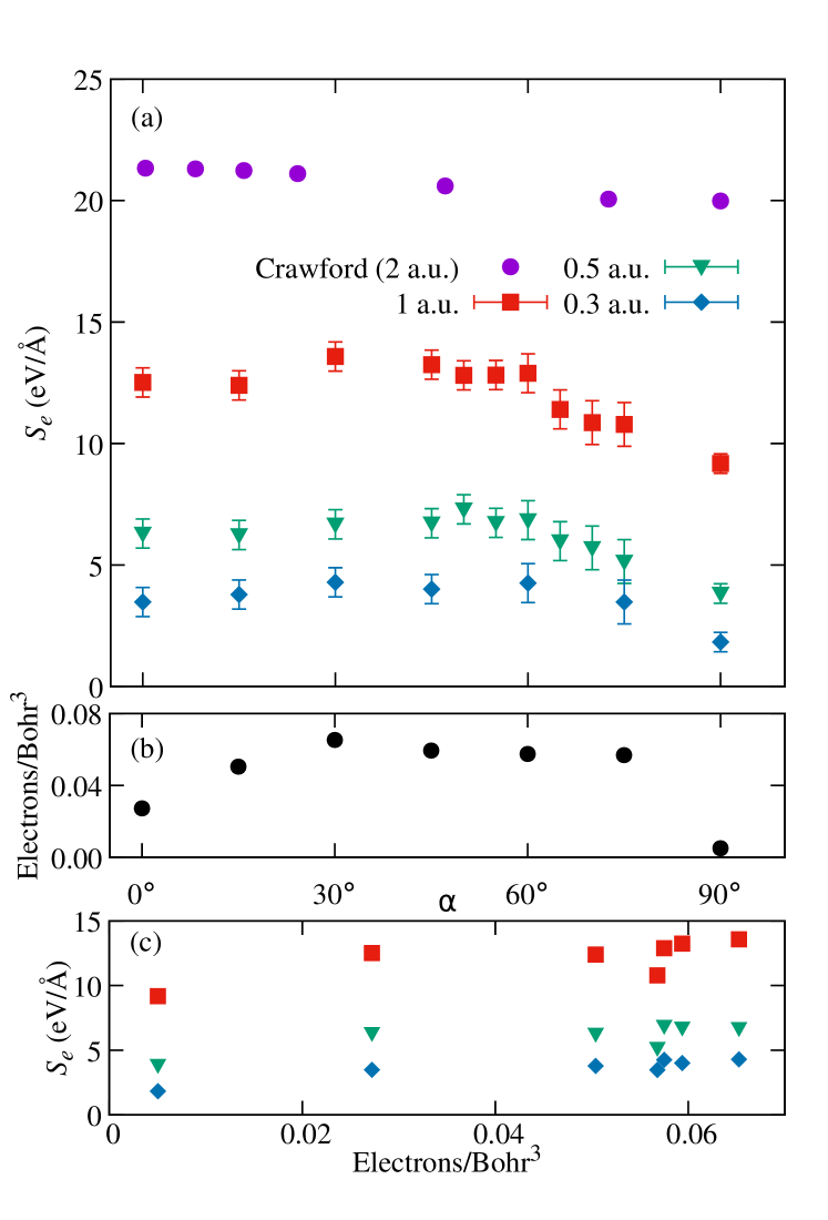
Figure 4 also includes the linear-response results of Crawford Crawford (1990) for comparison. The lowest velocity considered in that work is $v=2.0$ a.u., higher than those obtained in this work, which accounts for the higher overall $S_{e}$ . They also show a smaller angle dependence, of approximately 10% between a projectile moving along $\alpha=0^{\circ}$ and $90^{\circ}$ at 2 a.u., with smaller differences at higher projectile velocities; significantly lower than the equivalent difference for $v=1.0$ a.u. in our case. This is consistent with a further insensitivity with direction at high velocities Crawford (1990). Figure 9 of Shukri, Bruneval and Reining’s paper Shukri et al. (2016) also shows a small difference of up to 3% in $S_{e}$ between calculations with a projectile moving along $\alpha=0^{\circ}$ and $90^{\circ}$ in graphite at velocities between 0 and 4 a.u.. As discussed below, that work calculated the random electronic stopping power, which is averaged over all impact parameters, and so is not directly equivalent to the results in this paper.

III.2.1 Correlation of $S_{e}$ and electron density

Figure 4b shows the average electron density along a given trajectory versus $\alpha$ for comparison with $S_{e}(\alpha)$ , with the correlation between the two plotted in Figure 4c. The relationship between the electron density and $S_{e}$ is especially clear for the low velocities, with both $S_{e}$ and electron density increasing from $\alpha=0^{\circ}$ to $30^{\circ}$ , and the lowest $S_{e}$ at $90^{\circ}$ corresponding to the lowest electron density.

Under the scattering theory formalism developed by Echenique and others for jellium Wang et al. (1998); Wang and Nagy (1997); Winter et al. (2003); Echenique et al. (1986), the target electron density is space independent, a number $n$ , and the stopping power is a function $S_{e}(v,n)$ , which starts at zero for $n=0$ and increases with higher density. This results has been generalised to non-homogeneous electron systems, with the observation that the stopping power is larger when the projectiles traverse regions of higher density. This has been seen in previous work in various materials Ullah et al. (2015); Wang et al. (1998); Wang and Nagy (1997); Winter et al. (2003), and is used as a basic assumption in different contexts, as a local-density stopping approximation Winter et al. (2003). The results of the simulations presented here are consistent with this; between the graphitic layers the electron density is much lower than across the layers, and the higher the angle of the projectile relative to the $c$ axis the more time it spends in the lower electron density region between the layers. As a result the projectile interacts less with the electrons of the target and so the $S_{e}$ is lower, as seen in Figure 4, obtaining the minimum $S_{e}$ for $\alpha=90^{\circ}$ and the projectile moving midway between the planes, that is, the trajectory furthest from the carbon atoms and thus with the lowest electron density. It must be noted, however, that although the correlation is clear, it is not strict, as can be observed for $\alpha=75^{\circ}$ , although because of the orientation within the cell, the sampled trajectory both for the evaluation of $S_{e}$ and for the sampling of density values is poorer, which could be behind the larger deviation.

III.2.2 Channelling

The main channelling direction in graphite is along the $c$ axis ( $\alpha=0^{\circ}$ ), but the effect on $S_{e}$ is limited. Only a small depression can be observed for $S_{e}$ for $\alpha=0^{\circ}$ as compared with $15^{\circ}$ at low velocity. In Figure 4 it is visible for $v=0.3-0.5$ a.u., but it is clearly a much smaller effect than the one for $\alpha=90^{\circ}$ (parallel to graphitic layers) even if using perfect channelling trajectories, as trajectory 1 in Figure 1a. These results are consistent with the previous discussion, since the average density along that path does not reduce as much as for those parallel to and midway between graphitic planes.

Channelling in a crystal occurs when a projectile arrives into a channel in a trajectory within a small angle from the channel in a major crystal direction, and then moves along it undergoing small angle scattering, thereby moving along the channel. It is customarily expected that, as a result of the lack of nuclear collisions with the target material (beyond the small deflections implied by the channelling itself) and thereby reduced total energy loss of the projectile, the projectile travels further compared with a random direction in the crystal Lindhard (1965). For light projectiles and velocities above $\sim 0.1$ a.u., however, that effect becomes less important than the fact that $S_{e}$ itself is expected to be lower along a channelling direction, due to the lower average electron density in a channel; Schleife, Kanai and Correa Schleife et al. (2015) carried out TDDFT simulations of H in Al, comparing projectiles moving along channels with off-channelling directions, and found lower $S_{e}$ for a projectile moving along a channelling direction than along a random non-channelling direction. Channelling in graphite has only been experimentally observed when the projectile is moving along the c axis of graphite, perpendicular to the graphitic layers Elman et al. (1984); Iwata et al. (1975); Schroyen et al. (1986). That work used polycrystalline highly oriented pyrolytic graphite (HOPG), containing grain boundaries perpendicular to the graphitic layers, which would disrupt channelling between the layers. In HOPG, the basal planes are closely aligned, but alignment along the other axes is difficult to achieve. In theory, channelling would also be expected for a projectile travelling parallel to the graphitic layers, and the projectiles moving along $\alpha=90^{\circ}$ do show significantly lower $S_{e}$ .

III.2.3 Low velocity

The behavior of $S_{e}$ in the low velocity end of Figure 3 is remarkable. On the one hand, the simulations with the projectile moving at angles other than $90^{\circ}$ to the $c$ axis appear to show a threshold velocity of 0.02-0.06 eV below which, extrapolating the calculated data, $S_{e}$ appears to be either zero or very small on that scale. This is consistent with behavior seen in insulators Ullah et al. (2015) where the band gap results in a velocity threshold for $S_{e}$ . Graphite is effectively a semiconductor in the direction perpendicular to the graphitic layers, and, in that sense, this behavior would appear to be consistent with what is expected, at least qualitatively. In contrast, the obtained $S_{e}$ shown in Figure 3 for $\alpha=90^{\circ}$ , corresponding to a projectile moving midway between the graphitic layers, displays a very different behavior, with no apparent threshold but rather $S_{e}\propto v$ , but with a clear change of slope at $v\sim 0.3$ a.u. displayed by the lowest $S_{e}(v)$ graph in Figure 3.

III.3 Protons traveling between graphitic planes

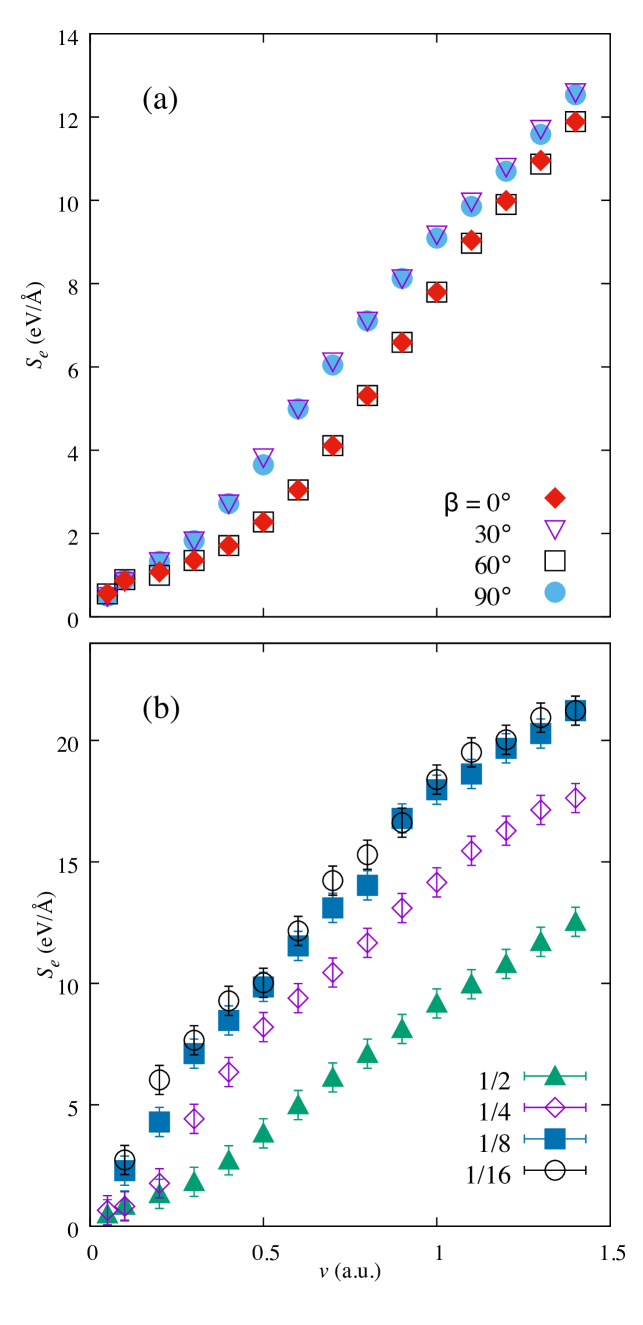
Figure 5 shows the behavior for trajectories parallel to the graphitic planes in more detail, with the $S_{e}(v)$ dependence for different orientations (Fig. 5a) and different impact parameters (proximity of the trajectory to the closest plane, Fig. 5b). Starting with Figure 5a, as discussed above, the $S_{e}$ is much lower at all velocities and all angles where the projectile is traveling parallel to the graphitic layers, as a result of the lower electron density between the layers. Due to the hexagonal symmetry of graphite, the trajectories $\beta=0^{\circ}$ and $\beta=60^{\circ}$ are crystallographically identical. $S_{e}(\beta)$ should therefore be periodic with a period of $60^{\circ}$ . It is expected to be symmetric around $0^{\circ}$ and $30^{\circ}$ , the values of $S_{e}$ for those $\beta$ ’s representing likely bounds for $S_{e}(\beta)$ . Figure 5a shows $S_{e}$ at 0 and $30^{\circ}$ as a function of velocity. The periodicity has been checked with the inclusion of results for $\beta=60^{\circ}$ and $90^{\circ}$ .

Figure 5(a) shows that the change of slope remains apparent for trajectories equidistant from two graphitic planes, irrespective of the $\beta$ angle, although for $\beta=0^{\circ}$ it happens at a slightly larger value of $v$ ( $v_{\mathrm{K}}\sim 0.4$ a.u.) than for $\beta=30^{\circ}$ ( $v_{\mathrm{M}}\sim 0.3$ a.u.). The former corresponds to the direction of the K-point in reciprocal space, while the latter to the M-point direction. Both values are close to the Fermi velocity of electrons around the Dirac cone ( $v_{F}=0.37$ a.u.), indicating that the change of slope is due to the onset of intra-cone electron-hole transitions contributing to the stopping. We base this observation on the fact that the electron-hole excitations generated by the moving projectile should respect the relationUllah et al. (2015)

\mathbf{v}\cdot\Delta\mathbf{k}=\Delta\epsilon

being $\Delta\mathbf{k}$ and $\Delta\epsilon$ the momentum and energy change of the electron, respectively, in the excitation, and $\mathbf{v}$ the projectile’s velocity. For $v<v_{F}$ , excitations can only be connecting across cones, while for $v\geq v_{F}$ the intra-cone channel is open.

A similar increase in the $S_{e}$ gradient at velocities between 0.3 and 0.5 a.u. has been seen in experiments for various systems: protons in Au Figueroa et al. (2007); Markin et al. (2008), He in Al Primetzhofer et al. (2011), and protons and He in Cu Markin et al. (2009), to name a few. The change in gradient for the Cu and Au experiments is suggested to be a result of interactions with the target’s 3 $d$ and 5 $d$ electrons in Cu and Au respectively at higher projectile velocities, where a minimum energy transfer is required for the excitation of $d$ electrons in both metals Figueroa et al. (2007). For He in Al, the slope change is thought to be due to charge-exchange processes between the target atoms and projectile Primetzhofer et al. (2011). This again suggests that the increase in gradient is due to additional energy loss mechanisms becoming accessible beyond a certain velocity, and which, in this case would correspond to the mentioned intra-cone transitions, meaning electron-hole-pair formation within the same band and small momentum transfer within the Brillouin zone, as the velocity approaches the Fermi velocity of the host.

III.3.1 Impact parameter dependence

The impact parameter dependence is shown in Figure 5b. It compares the $S_{e}$ for a projectile moving midway between the graphitic layers, and at positions $\frac{1}{4}$ , $\frac{1}{8}$ and $\frac{1}{16}$ of the interplanar distance from a graphitic layer, as shown in Fig. 2(b). The $S_{e}$ is higher at all velocities above 0.1 a.u. for the simulations closer to the graphite atoms, corresponding to the higher electron density closer to the graphitic layer. The gradient of the $S_{e}$ plot changes as the velocity increases, with a linear region between 0.5 and 1 a.u., and a slight decrease in gradient at higher velocities for both paths as the $S_{e}$ approaches a maximum. When the trajectories get closer to either atomic plane (Fig. 5b) $S_{e}$ significantly increases as compared to the mid-plane trajectory, and the clean two-slope structure of Figure 5(a) is lost, which should be attributed to scattering amplitude effects.

Trajectories perpendicular to the graphitic planes do not display significant impact-parameter dependence, however, unlike what is seen for trajectories parallel to the planes. $S_{e}$ increased only by 0.68 eV/Å when changing from trajectory 1 in Figure 1a to trajectory 4 at $v=0.5$ a.u..

The results of Shukri, Bruneval and Reining Shukri et al. (2016) investigated random electronic stopping power, defined as the $S_{e}$ averaged over all impact parameters. For the in-plane simulations, this is equivalent to averaging $S_{e}$ for all the trajectories at different distances from the graphitic layers. As Figure 5 shows, there is a significant increase in $S_{e}$ as the trajectory gets closer to a graphitic layer. The 3% difference between in-plane and out-of-plane simulations in $S_{e}$ seen by Shukri $et\ al.$ Shukri et al. (2016) is therefore consistent with the results in this work. Figure 3 shows the RESP from this work calculated as an average of the four impact parameters simulated for $\alpha=90^{\circ}$ . This simple average oversamples trajectories close to the graphitic layers (higher $S_{e}$ and therefore is an overestimate of the RESP; at high velocities we would expect all trajectories to be sampled equally..

IV Conclusions

Simulations of a hydrogen projectile traveling through graphite successfully reproduced experimental results, and provided new insights into the effect of the anisotropy of the graphite structure on electronic stopping power. The electronic stopping power is dependent on the direction of the projectile both relative to the graphitic layer normal and parallel to the layers. Although a clear correlation is found between the local electron density traversed by the trajectory in general, at low velocity $S_{e}$ displays varied behaviors depending on the direction and impact parameter. For channelling between planes and low density, a linear $S_{e}$ is observed, consistent with (semi)metallic electron conduction, but which changes slope when the projectile velocity reaches the Fermi velocity of the target. For trajectories with dominant component perpendicular to the graphitic plane, a threshold is observed at $v\sim 0.05$ a.u., consistent with poor electron conduction between planes.

This work investigates the initial stages of radiation damage; for a fuller understanding of the processes that lead to the final observed radiation damage, simulations must be carried out at longer time scales and with larger simulation sizes. Progression from $S_{e}$ calculations can be envisaged by following the diffusion of the excess electronic energy, and its thermalisation to the ionic motion. In addition to the technical challenges from increased simulation size, theoretical challenges also exist, as Ehrenfest dynamics are known to be inadequate for the simulation of this thermalisation. Beyond Ehrenfest approximations are far more computationally demanding, and therefore present a significant challenge but would offer valuable insights into the progress of stopping processes and the mechanisms of radiation damage.

Acknowledgements.

The authors would like to thank P. Alemany for useful discussions on this work. J. H. would like to thank R. Ullah for his technical help in the initial stages of this work. This work was performed using resources provided by the Cambridge Tier-2 system operated by the University of Cambridge Research Computing Service http://www.hpc.cam.ac.uk , funded by Engineering and Physical Sciences Research Council Tier-2 (capital Grant No. EP/P020259/1), and DiRAC funding from the Science and Technology Facilities Council www.dirac.ac.uk . J. H. would like to acknowledge the EPSRC Centre for Doctoral Training in Computational Methods for Materials Science for funding under Grant No. EP/L015552/1.

Appendix

This section describes the testing carried out to generate the initial simulation parameters. The pseudopotentials of C and H were generated using the scheme of Troullier and Martins Troullier and Martins (1991) and the corresponding parameters are shown in Table 1.

Table 1: Pseudopotential radii for each angular-momentum channel of C and H. Lengths are in Bohr.

Species	$s$	$p$	$d$	$f$
C (2 $s^{2}$ 2 $p^{2}$ )	1.49	1.50	1.56	1.56
H (1 $s^{2}$ )	1.25	1.25	1.25	1.25

Table 2 gives the parameters needed for the generation of the basis set used in this work, following the procedures described in Ref. 63. The polarisation orbitals were generated by applying an electric field to the orbital according to the procedure implemented in SIESTA and described in Ref. Soler et al., 2002.

Table 2: Cutoff radii

r(\zeta_{1})

and

r(\zeta_{2})

in Bohr of the first and second

\zeta

functions of C and H.

Species	$n$	$l$	$r(\zeta_{1})$	$r(\zeta_{2})$
C	2	0	4.192	3.432
	2	1	4.870	3.475
H	1	0	4.828	3.855

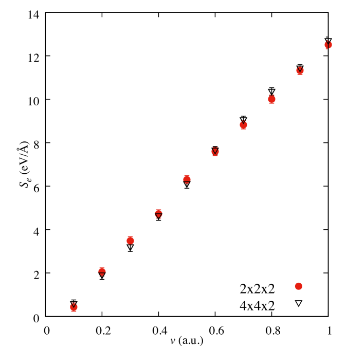
A periodic supercell of $2\times 2\times 2$ graphite unit cells was used, containing 32 C atoms and a single H atom, with lattice parameters of $a$ = 2.461 Å, $c$ = 6.573 Å. A number of supercell sizes were tested to confirm that the supercell used was sufficiently large to give good quality results. Figure 6 compares the electronic stopping power for a projectile moving perpendicular to the graphitic layers in $2\times 2\times 2$ and a $4\times 4\times 2$ supercells containing 33 and 129 atoms. There is no significant difference between the electronic stopping powers in this velocity range for the two supercell sizes, confirming that the $2\times 2\times 2$ supercell is sufficient to produce accurate results.

A single k-point ( $\Gamma$ ) was used for the Brillouin zone integrations, after testing a ground state calculation with up to 90 k-points for convergence and simulation time. The difference between $S_{e}$ for one k-point and 96, for trajectory number 1 and $v=1$ a.u., was only 0.2 eV/Å. A timestep of 1 attosecond was used for the low velocity simulations up to 1 a.u., and of 0.1 attoseconds for simulations above 1 a.u. after testing for the stability of the Crank-Nicolson integrator algorithm and the energy change in a TDDFT simulation. The plane-wave energy cutoff for real space integration was tested between 50 and 400 Ry; the total energy converged at around 150 Ry, and a 200 Ry cutoff energy was finally used in the simulations.

References

Was (2007) G. S. Was, Fundamentals of Radiation Materials Science (Springer-Verlag, 2007).
Begg et al. (2011) A. C. Begg, F. A. Stewart, and C. Vens, Nat Rev Cancer 11, 239 (2011).
Eisen et al. (1972) F. H. Eisen, G. J. Clark, J. B⊘ttiger, and J. M. Poate, Radiation Effects 13, 93 (1972).
Dygo et al. (1994) A. Dygo, M. A. Boshart, L. E. Seiberling, and N. M. Kabachnik, Phys. Rev. A 50, 4979 (1994).
dos Santos et al. (1997) J. H. R. dos Santos, P. L. Grande, M. Behar, H. Boudinov, and G. Schiwietz, Phys. Rev. B 55, 4332 (1997).
Käferböck et al. (1997) W. Käferböck, W. Rössler, V. Necas, P. Bauer, M. Peñalba, E. Zarate, and A. Arnau, Phys. Rev. B 55, 13275 (1997).
Softky (1961) S. D. Softky, Phys. Rev. 123, 1685 (1961).
Seltzer and Berger (1982) S. M. Seltzer and M. J. Berger, The International Journal of Applied Radiation and Isotopes 33, 1189 (1982).
Crawford (1990) O. H. Crawford, Phys. Rev. A 42, 1390 (1990).
Shukri et al. (2016) A. A. Shukri, F. Bruneval, and L. Reining, Phys. Rev. B 93, 035128 (2016).
Echenique et al. (1981) P. Echenique, R. Nieminen, and R. Ritchie, Solid State Communications 37, 779 (1981).
Echenique et al. (1986) P. M. Echenique, R. M. Nieminen, J. C. Ashley, and R. H. Ritchie, Phys. Rev. A 33, 897 (1986).
Ferrell and Ritchie (1977) T. L. Ferrell and R. H. Ritchie, Phys. Rev. B 16, 115 (1977).
Lindhard (1954) J. Lindhard, Matematisk-fysiske Meddelelser 28 (1954).
Echenique et al. (1990) P. Echenique, F. Flores, and R. Ritchie, Solid State Phys. 43, 229 (1990).
Sigmund (2014) P. Sigmund, Particle Penetration and Radiation Effects Volume 2 (Springer International Publishing, 2014).
Mason et al. (2007) D. R. Mason, J. le Page, C. P. Race, W. M. C. Foulkes, M. W. Finnis, and A. P. Sutton, J. Phys. Condens. Matter 19, 436209 (2007).
Race et al. (2010) C. P. Race, D. R. Mason, M. W. Finnis, W. M. C. Foulkes, A. P. Horsfield, and A. P. Sutton, Rep. Prog. Phys. 73, 116501 (2010).
Krasheninnikov et al. (2007) A. V. Krasheninnikov, Y. Miyamoto, and D. Tománek, Phys. Rev. Lett. 99, 016104 (2007).
Pruneda et al. (2007) J. M. Pruneda, D. Sánchez-Portal, A. Arnau, J. I. Juaristi, and E. Artacho, Phys. Rev. Lett. 99, 235501 (2007).
Zeb et al. (2012) M. A. Zeb, J. Kohanoff, D. Sánchez-Portal, A. Arnau, J. I. Juaristi, and E. Artacho, Phys. Rev. Lett. 108, 225504 (2012).
Correa et al. (2012) A. A. Correa, J. Kohanoff, E. Artacho, D. Sánchez-Portal, and A. Caro, Phys. Rev. Lett. 108, 213201 (2012).
Zeb et al. (2013) M. A. Zeb, J. Kohanoff, D. Sánchez-Portal, and E. Artacho, Nucl. Instrum. Meth. B 303, 59 (2013).
Ojanperä et al. (2014) A. Ojanperä, A. V. Krasheninnikov, and M. Puska, Phys. Rev. B 89, 035120 (2014).
Caro et al. (2015) A. Caro, A. A. Correa, A. Tamm, G. D. Samolyuk, and G. M. Stocks, Phys. Rev. B 92, 144309 (2015).
Schleife et al. (2015) A. Schleife, Y. Kanai, and A. A. Correa, Phys. Rev. B 91, 014306 (2015).
Ullah et al. (2015) R. Ullah, F. Corsetti, D. Sánchez-Portal, and E. Artacho, Phys. Rev. B 91, 125203 (2015).
Caro et al. (2017) M. Caro, A. A. Correa, E. Artacho, and A. Caro, Sci. Rep. 7, 2045 (2017).
Bubin et al. (2012) S. Bubin, B. Wang, S. Pantelides, and K. Varga, Phys. Rev. B 85, 235435 (2012).
Lee, Cheng-Wei and Schleife, André (2018) Lee, Cheng-Wei and Schleife, André, Eur. Phys. J. B 91, 222 (2018).
Yost et al. (2017) D. C. Yost, Y. Yao, and Y. Kanai, Phys. Rev. B 96, 115134 (2017).
Chung (2002) D. D. L. Chung, J. Mater. Sci. 37, 1475 (2002).
Cazaux (1970) J. Cazaux, Solid State Commun. 8, 545 (1970).
Yagi et al. (2004) E. Yagi, T. Iwata, T. Urai, and K. Ogiwara, J. of Nucl. Mater. 334, 9 (2004).
Tsolakidis et al. (2002) A. Tsolakidis, D. Sánchez-Portal, and R. M. Martin, Phys. Rev. B 66, 235416 (2002).
Ullah et al. (2019) R. Ullah, A. Garaizar, F. Corsetti, J. Kohanoff, D. Sanchez-Portal, and E. Artacho, , forthcoming (2019).
Soler et al. (2002) J. M. Soler, E. Artacho, J. D. Gale, A. García, J. Junquera, P. Ordejón, and D. Sánchez-Portal, J. Phys. Condens. Matter 14, 2745 (2002).
Artacho et al. (2008) E. Artacho, E. Anglada, O. Diéguez, J. D. Gale, A. García, J. Junquera, R. M. Martin, P. Ordejón, J. M. Pruneda, D. Sánchez-Portal, and J. M. Soler, J. Phys. Condens. Matter 20, 064208 (2008).
(39) S. Froyen, N. J. Troullier, J. L. Martins, L. C. Balbás, J. M. Soler, and A. Garcia, “ATOM, a program for DFT calculations in atoms and pseudopotential generation,” https://departments.icmab.es/leem/siesta/Pseudopotentials/Code/downloads.html.
Troullier and Martins (1991) N. Troullier and J. L. Martins, Phys. Rev. B 43, 1993 (1991).
Ullah et al. (2018) R. Ullah, E. Artacho, and A. A. Correa, Phys. Rev. Lett. 121, 116401 (2018).
Ceperley and Alder (1980) D. M. Ceperley and B. J. Alder, Phys. Rev. Lett. 45, 566 (1980).
Perdew and Zunger (1981) J. P. Perdew and A. Zunger, Phys. Rev. B 23, 5048 (1981).
Kohn and Sham (1965) W. Kohn and L. J. Sham, Phys. Rev. 140, A1133 (1965).
Runge and Gross (1984) E. Runge and E. K. U. Gross, Phys. Rev. Lett. 52, 997 (1984).
Pietsch et al. (1976) W. Pietsch, U. Hauser, and W. Neuwirth, Nucl. Instrum. Methods 132, 79 (1976).
(47) J. K. Tomfohr and O. F. Sankey, Phys. Status Solidi B 226, 115.
Artacho and O’Regan (2017) E. Artacho and D. D. O’Regan, Phys. Rev. B 95, 115155 (2017).
Deasy (1994) J. Deasy, Med. Phys. 21, 709 (1994).
Wang et al. (1998) N.-P. Wang, I. Nagy, and P. M. Echenique, Phys. Rev. B 58, 2357 (1998).
Wang and Nagy (1997) N.-P. Wang and I. Nagy, Phys. Rev. A 56, 4795 (1997).
Winter et al. (2003) H. Winter, J. I. Juaristi, I. Nagy, A. Arnau, and P. M. Echenique, Phys. Rev. B 67, 245401 (2003).
Lindhard (1965) J. Lindhard, Matematisk-fysiske Meddelelser 14 (1965).
Elman et al. (1984) B. S. Elman, G. Braunstein, M. S. Dresselhaus, G. Dresselhaus, T. Venkatesan, and B. Wilkens, J. Appl. Phys. 56, 2114 (1984).
Iwata et al. (1975) T. Iwata, K.-I. Komaki, H. Tomimitsu, K. Kawatsura, K. Ozawa, and K. Doi, Radiation Effects 24, 63 (1975).
Schroyen et al. (1986) D. Schroyen, M. Bruggeman, I. Dezsi, and G. Langouche, Nucl. Instrum. Meth. B 15, 341 (1986).
Figueroa et al. (2007) E. A. Figueroa, E. D. Cantero, J. C. Eckardt, G. H. Lantschner, J. E. Valdés, and N. R. Arista, Phys. Rev. A 75, 010901(R) (2007).
Markin et al. (2008) S. N. Markin, D. Primetzhofer, S. Prusa, M. Brunmayr, G. Kowarik, F. Aumayr, and P. Bauer, Phys. Rev. B 78, 195122 (2008).
Primetzhofer et al. (2011) D. Primetzhofer, S. Rund, D. Roth, D. Goebl, and P. Bauer, Phys. Rev. Lett. 107, 163201 (2011).
Markin et al. (2009) S. N. Markin, D. Primetzhofer, M. Spitz, and P. Bauer, Phys. Rev. B 80, 205105 (2009).
(61) http://www.hpc.cam.ac.uk, .
(62) www.dirac.ac.uk, .
Junquera et al. (2001) J. Junquera, O. Paz, D. Sánchez-Portal, and E. Artacho, Phys. Rev. B 64, 235111 (2001).